Correlation functions, Bell’s inequalities and the fundamental conservation laws

Abstract

I derive the correlation function for a general theory of two-valued spin variables that satisfy the fundamental conservation law of angular momentum. The unique theory-independent correlation function is identical to the quantum mechanical correlation function. I prove that any theory of correlations of such discrete variables satisfying the fundamental conservation law of angular momentum violates the Bell’s inequalities. Taken together with the Bell’s theorem, this result has far reaching implications. No theory satisfying Einstein locality, reality in the EPR-Bell sense, and the validity of the conservation law can be constructed. Therefore, all local hidden variable theories are incompatible with fundamental symmetries and conservation laws. Bell’s inequalities can be obeyed only by violating a conservation law. The implications for experiments on Bell’s inequalities are obvious. The result provides new insight regarding entanglement, and its measures.

PACS Numbers: 03.65.Ta, 03.65.Ud

The main result of this paper is the proof that a general physical theory of correlations of two-valued spin projections violate the Bell’s inequalities if the theory satisfies the conservation law for angular momentum on the average. The proof is applicable to local hidden variable theories, as well as to other theories like the non-local hidden variable theories, and to quantum mechanics itself, with the only assumption that they respect the conservation law for the ensemble average. The proof follows from the result that any such theory predicts a unique correlation function that is in fact identical to the quantum mechanical correlation function. Since such fundamental conservation laws have their origin in space-time symmetries, and since we expect that the only viable theories of the physical world are those satisfying these conservation laws, this result has far reaching significance. The physical situation we consider is the measurements of spin-projections of spin-half particles or photons with their total angular momentum zero. The proof is applicable to other values of total angular momentum.

A local hidden variable theory is a classical statistical theory meant to replace quantum mechanics. Such theories were proposed with the hope that one could preserve classical notions like locality, and reality of events and history in space and time, and yet reproduce the statistical results of quantum mechanics [1, 2]. The randomness in the measured results of an observable in such theories is mapped to the random values taken by certain hidden or unobservable classical variables. John Bell’s analysis of local hidden variable theories resulted in the celebrated Bell’s inequalities [2]. These represent an upper limit on the correlation expected in such theories between results of measurements on separated correlated quantum systems. In the standard formulations, the correlation and its upper limit in a local hidden variable theory are typically smaller than what is predicted in the quantum mechanical description, for a wide range of settings of the measurement apparatus. Thus, quantum mechanical correlations violate the Bell’s inequalities.

Several experiments have been done in the past, and several are in planning and execution to test the Bell’s inequalities, and to thereby test the viability of local hidden variable theories [3]. Essentially all experiments to date find that the Bell’s inequalities are violated, and that the measured correlations are in fact larger than the upper limit specified by the Bell’s inequalities. The experiments also confirm with high precision that the quantum mechanical prediction for the correlation is what is favoured.

Bell’s derivation of the inequalities assumed Einstein locality, and local hidden variables that could determine outcomes of measurements, and he dealt with two-valued observables. The physical setting is that of two observers $A$ and $B$ making measurements on two correlated particles individually at space-like separated regions with time information such that these results can be correlated event by event.

Locality in hidden variable theories is represented by functional restrictions on the outcomes $A$ and $B$ of measurements at the two locations.

$$A(\mathbf{a,h})=\pm 1,\quad B(\mathbf{b,h})=\pm 1$$ (1)

$A$ and $B$ denote the outcomes $+1$ or $-1$ of measurements $A$ and $B,$ and $\mathbf{a}$ and $\mathbf{b}$ denote the settings of the analyzer or the measurement apparatus for the first particle and the second particle respectively. $\mathbf{h}$ are hidden variables associated with the outcomes. The Bell correlation function [2] is of the form

$$P(\mathbf{a},\mathbf{b})=\int d\mathbf{h}\rho(\mathbf{h})A(\mathbf{a,h})B(\mathbf{b,h}),\mathrm{{where}\int d\mathbf{h}\rho(\mathbf{h})=1}$$ (2)

This is an average over the product of the measurement results. The experimenter calculates the observed correlation using the formula

$$P(\mathbf{a},\mathbf{b})=\frac{1}{N}\sum(A_{i}B_{i})$$ (3)

from the observed outcomes $A_{i}$ and $B_{i}.$ The essence of Bell’s theorem is that the function $P(\mathbf{a},\mathbf{b})$ has distinctly different dependences on the relative angle between the analyzers for a local hidden variable description and for quantum mechanics. If $\mathbf{a}$ and $\mathbf{a}^{\prime}$ are two settings of the apparatus at $A,$ and $\mathbf{b},\mathbf{b}^{\prime}$ are settings at $B,$ then it was shown [2] that the combination of correlations

$$M_{LHVT}=\left|P(\mathbf{a},\mathbf{b})-P(\mathbf{a},\mathbf{b}^{\prime})\right|+\left|P(\mathbf{a}^{\prime},\mathbf{b}^{\prime})+P(\mathbf{a}^{\prime},\mathbf{b})\right|\leq 2$$ (4)

The quantum mechanical correlation for the same experiment is given by

$$P(\mathbf{a},\mathbf{b})_{QM}=-\mathbf{a}\cdot\mathbf{b}$$ (5)

This is the expectation value of the operator $\sigma_{1}\cdot\mathbf{a\otimes\sigma}_{2}\cdot\mathbf{b}$ for the singlet state (When expressed in units of $\hbar/2$. In terms of values of the projections of spin, the correlation function is $P(\mathbf{a},\mathbf{b})_{QM}=-\mathbf{a}\cdot\mathbf{b~{}\hbar}^{2}/4$). There are several combinations of the set $\left\{\mathbf{a},\mathbf{a}^{\prime},\mathbf{b},\mathbf{b}^{\prime}\right\}$ for which $M_{QM}$ exceeds $M_{LHVT}$ of local hidden variable theories. Thus quantum mechanical correlations violates Bell’s inequalities.

In what follows, we start with the assumption the validity of the fundamental conservations laws, like the conservation of angular momentum, on the average (for probabilities) and calculate the general correlation function that is allowed for two-valued observables. We make no assumptions on locality, or on reality in the Einstein-Podolsky-Rosen sense. Thus, our assumption is the minimal one that is expected to be satisfied by any theory consistent with the fundamental symmetries like rotational invariance, with or without hidden variables. Therefore the results are valid for a wide class of theories including local hidden variable theories, non-local theories, and quantum mechanics.

The proof is generally valid for theories satisfying following criteria.

1. The theory deals with observations on two particles $A$ and $B$ that show discrete outcomes, for a particular measurement like the projection of the angular momentum. Then the product of observed values in one joint measurement for any relative settings of the apparatus are quantized and ranges from $+S^{2}$ to $-S^{2}.$ This is of course due to the fact that each subsystem can take only values from $+S$ to $-S,$ in steps of $1.$ Thus the theory is not dealing with standard classical measurements where any value between $+S$ to $-S$ is allowed. For the special case of two-valued outcomes, $A=\pm 1,\quad B=\pm 1,$ in units is $S.$ This is the case considered by Bell.

2. The theory of correlations obeys the conservation of angular momentum on the average over the ensemble, and for the case of singlet state, $S_{Total}=0,$ there is rotational invariance. Note that this is a weak assumption, since we do not insist on the validity of the conservation law for individual events.

The correlation function allowed by the basic assumption of validity of conservation law is unique, and surprisingly it is identical to the quantum mechanical correlation function. Therefore, a physical system with discrete observable values can show correlations different from what is predicted by quantum mechanics only by violating a fundamental conservation law! It is possible to extend this analysis to continuous variables, though here we focus on the experimentally favoured physical systems with discrete outcomes, as originally considered by Bell. The second criterion is the main assumption, physically well motivated, in the proof that follows. Since the main assumption is applied only for ensemble averages and not for individual events, I do not make any explicit assumption on locality or reality.

To show the inseparable relation between the validity of the conservation law on the average and the correlation functions in the most transparent way, first I will derive the correlation function for the spin-1/2 two-particle system whose total angular momentum is zero. In quantum mechanics this corresponds to the two-particle singlet state. We will then derive the general result for higher spin singlet states.

It is  well known that rotational invariance of the singlet state already demands that the correlation function is proportional to $\mathbf{a}\cdot\mathbf{b,}$ though not enough attention has been paid to the consequence that any other correlation function will violate the basic symmetry and conservation law.

Consider a set of measurements in which the direction at $A$ is fixed as $\mathbf{a}$ and that at $B$ is fixed as $\mathbf{b}$. Each individual measurement in any direction gives either $+1$ or $-1$ (in unit of $\hbar/2$). Prepare two subsets of results on the location $A$; one subset containing only $+1$ and the other containing only $-1.$ For the initial two-particle system with total zero angular momentum, there will be equal number of $+1$ and $-1$ at $A$ and $B$. The average angular momentum in each subset is given by the average of the individual values. For the first subset at $A$ this is simply $+1$ and for the second subset, it is $-1$ (both in units of $\hbar/2$). There will be two correlated subsets at $B$, whose individual averages will depend on the setting at $B$. For this one has to use the temporal information for deciding which measurement at $B$ needs to be correlated with a particular measurement at $A$. (The situation is symmetric – we can start with two subsets of $B$, and then examine the correlated subsets of $A$). If both analyzers were set for the same direction, $\mathbf{a=b,}$ the (anti) correlation is perfect according to the conservation of angular momentum, and the average angular momentum at $B$ would be $-1.$ For an arbitrary direction $\mathbf{b}$ at $B,$ conservation of angular momentum then predicts that the average of the angular momentum measured for the second particle, correlated with the $+\hbar/2$ values of the first particle, should be simply the vectorial projection of $-\hbar/2$ onto the direction $\mathbf{b}$, or just $-\cos(\theta)$ in unit of $\hbar/2,$ where $\theta$ is the angle between the measurement directions (see figure 1).

It is perhaps important to stress this obvious point further, with a proof, to preempt a possible confusion. For individual measurements of the two-point correlation, the conservation law cannot be invoked, since only the conditional probabilities are predicted by quantum mechanics. Therefore, measurement of $+1$ on one particle still leaves the outcome on the other random, with only the probability fixed by the theory. The situation for averages is very different. If the average spin projection for the $+$subset on the particles at $A$ gives $S_{A}=+1,$ and if the average at $B$ is $S_{B}(\theta)$ for the setting of the analyzer at an angle $\theta,$ the component of average angular momentum at $A$ in the direction identical to the setting at $B$ is

$$S_{A,\theta}=S_{A}\cos(\theta)=\cos(\theta)$$ (6)

Conservation of angular momentum implies that the total angular momentum in any direction is zero since the initial angular momentum is zero. Therefore

$$S_{tot}=S_{A,\theta}+S_{B}(\theta)=\cos(\theta)+S_{B}(\theta)=0$$ (7)

This is independent of the theory, and necessarily implies that for any theory and for experimental data that respect the conservation law, $S_{B}(\theta)=-\cos(\theta),$ given that average $S_{A}=+1.$ What is important is to note that this statement uses only the vectorial properties of the mechanical quantity, the average angular momentum, and does not involve counter-factual arguments as it would for individual measurements. Therefore, irrespective of the theoretical description, angular momentum conservation will be violated if $S_{B}(\theta)\neq-\cos(\theta)$ when $S_{A}=+1.$

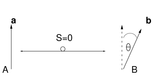
Figure 1: Diagram explaining the settings of the anlayzers. Since the average angular momentum is a vectorial quantity, the average correlation at angle $\theta$ is $-\cos(\theta),$ when the source has zero angular momentum.

Similarly, for the subset with results $-1$ for $A$, the average of the correlated events at $B$ will be the projection of the angular momentum $+1$, or $+\cos(\theta).$ The correlation of the angular momentum between $A$ and $B$ in both cases is the average of the corresponding products in the two subsets, $[-1_{A}\times\cos(\theta)_{B}+1_{B}\times-\cos(\theta)_{A}]/2,$ which is $-\cos(\theta).$ Therefore the correlation for the entire set is also $-\cos(\theta)$ or $P(\mathbf{a},\mathbf{b})=-\mathbf{a}\cdot\mathbf{b.}$

It is worth listing the steps clearly leading to the theory-independent correlation function that follows from the conservation law. The projection of the classical angular momentum vector in a direction that is rotated by angle $\theta$ is just $\cos(\theta).$ In a situation in which individual measurements give discrete values $+1$ and $-1,$ the average angular momentum still preserves this relation. A set of particles with angular momentum is $+1$ in a particular direction will show an average angular momentum $\cos(\theta)$ in a direction rotated by $\theta.$

The correlation function of a set of measurements on two particles is

$$P(\mathbf{a},\mathbf{b})=\frac{1}{N}\sum(A_{i}B_{i})$$ (8)

We consider the situation when the initial angular momentum of the two particles together is zero. Since $A_{i}$ and $B_{i}$ take values of $+1$ or $-1$, we group the values such that all $A_{i}$ are $+1$ in the first group and all $A_{i}$ are $-1$ in the second. Of course the $B_{i}$ are mixed in both groups. Then the summation index, which is scrambled now due to regrouping, is relabelled from $1$ to $N$ again, preserving the relative order and thus the correlation. We  get

$$P(\mathbf{a},\mathbf{b})_{C}=\frac{1}{N}\sum(A_{i}B_{i})=\left\langle\left(\frac{1}{N_{A+}}\sum_{j=1}^{N/2}+1.(B_{j})+\frac{1}{N_{A-}}\sum_{j=(N/2)+1}^{N}-1.(B_{j})\right)\right\rangle$$ (9)

We have used the subscript $C$ to indicate that this correlation function assumes the validity of the conservation law. The first term is the conditional average of $B_{j}$ given $A_{j}=1,$ and the second term is the average of $B_{j}$ given $A_{j}=-1.$ $N_{A+}=N_{A-}=N/2.$ Then we get, using only the conservation law for the averages,

$$P(\mathbf{a},\mathbf{b})_{C}=\frac{1}{2}\left(-\cos(\theta\right)-\cos(\theta))=-\cos(\theta)$$ (10)

This is same as the quantum mechanical correlation function $P(\mathbf{a},\mathbf{b})_{QM}.$ We have proved that the correlation function $-\cos(\theta)$ and thus $P(\mathbf{a},\mathbf{b})_{QM}$ is a consequence of the conservation of angular momentum. The correlation function represents the conservation law, and follows uniquely and directly from it.

The combination

$$M_{C}=\left|P(\mathbf{a},\mathbf{b})-P(\mathbf{a},\mathbf{b}^{\prime})\right|+\left|P(\mathbf{a}^{\prime},\mathbf{b}^{\prime})+P(\mathbf{a}^{\prime},\mathbf{b})\right|$$ (11)

for the theory of correlations satisfying the fundamental conservation law is thus identical to $M_{QM}$ since $P(\mathbf{a},\mathbf{b})_{C}=P(\mathbf{a},\mathbf{b})_{QM}.$ It follows that $M_{C}$ can exceed $M_{LHVT}$ for several combinations $\left\{\mathbf{a},\mathbf{a}^{\prime},\mathbf{b},\mathbf{b}^{\prime}\right\}.$

This derivation of the unique correlation function for the spin-1/2 two-particle system from the conservation of angular momentum immediately implies that any other correlation function with a dependence on the relative angle other than $-\cos(\theta)$ violates the law of conservation of angular momentum. Since the Bell’s inequalities can be obeyed only when the correlation function is different from the quantum mechanical correlation $-\mathbf{a}\cdot\mathbf{b,}$ it follows that a local hidden variable theory does not respect the law of conservation of angular momentum. In order to get a deviation from the correlation function $P(\mathbf{a},\mathbf{b})_{C}=-\mathbf{a}\cdot\mathbf{b=}$ $P(\mathbf{a},\mathbf{b})_{QM},$ the conservation law for angular momentum has to be violated. This completes the proof that a general theory of correlations of discrete two-valued variables will violate the Bell’s inequalities if the theory respects the fundamental conservation law of angular momentum on the average.

The generalization to higher spins is straightforward. For a spin-$S$ entangled singlet state, there will be $2S+1$ different possibilities for measurement results, $+S,+(S-1)..0..-(S-1),-S.$ All of these occur with equal probability, due to rotational invariance, and we group the measurements at $A$ as earlier in this sequence. For a specific group, say with $(S-n)$ as the projection, conservation of angular momentum implies that the average of the angular momentum at $B$ is just the vector projection of the opposite angular momentum, $-(S-n)\cos(\theta).$ Then the correlation for that group is

$$P(S,\theta)=-(S-n)^{2}\cos(\theta)$$ (12)

The same correlation will be observed also for the results $-(S-n)$ at $A.$ For the ‘$0$’ state, the correlation (average of the angular momentum correlation) is zero. Therefore, the average of all the two-point measurements is

$$P(\mathbf{a},\mathbf{b)}_{C} \mathbf{=}\frac{-\cos(\theta)\left(S^{2}+(S-1)^{2}+...0+...(S-1)^{2}+S^{2}\right)}{2S+1}$$

$$=-2\cos(\theta)\left(S^{2}+(S-1)^{2}+...0\right)/2S+1$$

$$=-2\cos(\theta)S(S+1)(2S+1)/6(2S+1)$$

$$=-\cos(\theta)S(S+1)/3$$ (13)

This is exactly the quantum mechanical correlation function $P(\mathbf{a},\mathbf{b)}_{QM}$ for the spin-$S$ singlet state [4]. Thus, the physically valid correlation function can be uniquely derived from the conservation law, and any other correlation function is incompatible with the requirement of conservation of angular momentum on the average. Note that this gives the correct $P(\mathbf{a},\mathbf{b)=}-\cos(\theta)/4$ for the spin-$1/2$ case, or just $-\cos(\theta)$ when  the observable values are taken as $+1$ and $-1$ instead of $+1/2$ and $-1/2.$

To be more explicit and precise about the amount of departure from the conservation law, let us see what the angular dependence of the Bell correlation function for local hidden variable theory looks like. This dependence can be derived using the assumption of locality and observing that the joint probabilities obey the separability of probabilities in the local hidden variable theories (This is done and discussed in detail in Bell’s writings; see for example ref. [5]). If the angle of one of the analyzers is suddenly changed, the correlation function has to change, and since there is no information available on the instantaneous setting of the second spatially separated analyzer, this change is to be composed of individual changes that depends separably on the individual angular setting of each analyzer. This shows that the correlation function changes linearly with angle (Fig. 2) [5]. If the correlation function obeys the constraint that for $\theta=0$ the correlation is perfect and for $\theta=\pi/2$ the correlation is zero for the spin-half case, the function is linear in the entire range. We see that such a correlation function does not respect the conservation of angular momentum of the total state on the average. Note that it is not possible to attribute the missing angular momentum to the hidden variables, since the theory is local and perfect conservation is seen for special angular settings.

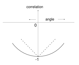
Figure 2: Diagram showing the different dependences of the correlation function from conservation law (solid curve, same as the QM correlation function) and the Bell Correlation function, on relative angle. The linear change in correlation (dotted lines) is a characteristic of local hidden vaiable theories of the type discussed by Bell. It violates the requirement of conservation of angular momentum as explained in the text.

The implications of this result to any experiment attempting to test the Bell’s inequalities are obvious. All such experiments are testing for the possible validity of theories that are incompatible with the fundamental conservation laws. Given that these conservation laws are consequences of symmetries, independent of any theoretical formulation, there is no surprise that experimentally measured correlations follow the expression $P(\mathbf{a},\mathbf{b})_{C}=-\mathbf{a}\cdot\mathbf{b.}$ Any other correlation indicates a violation of the conservations law on the average. If this result were known before such experimental attempts started, the attitude towards such tests was likely to be very different. In any case, it is clear that any expectation of large deviation from this correlation function, required to obey the Bell’s inequalities, is physically unfounded and in dissonance with the good symmetries.

This result reinforces the statements made earlier in ref. [7] that entanglement in such cases is the general superposition with the constraint of conservation law of angular momentum. The conservation law is what is encoded in the relative phase, and in entanglement. Thus the fidelity with which the conservation law is preserved is directly related to the measure of entanglement. Processes like decoherence diffuses the individual phase and thus the relative phase, slowly washing out the fidelity of the conservation law (preserved however when the total system including the interacting environment is considered) and hence the entanglement fidelity. With this insight, it is much easier to understand the subtleties of quantum entanglement. Applications of this insight will be discussed elsewhere.

In summary, I have shown that a unique correlation function is associated with a general theory of correlations of discrete two-valued variables if the theory respects the fundamental conservation law of angular momentum on the average. This correlation function turns out to be identical to the quantum mechanical correlation function for the same experimental situation. I have also shown that such a correlation function and therefore theories of correlations that respect the conservation law violate the Bell’s inequalities. Measured correlations of spin projections can obey the Bell’s inequality only by violating the conservation law of angular momentum. A theory of correlations satisfying Einstein locality and EPR reality satisfies the Bell’s inequality and a theory that satisfies the fundamental conservation law violates the inequality. Therefore, a theory of correlations satisfying Einstein locality, reality in the Einstein-Bell sense, and the validity of the fundamental conservation law cannot be constructed. Some discussion on the mutual compatibility of the conservation laws and Einstein locality can be found in ref. [6, 7]. A generalization of these results to continuous observables is in progress.

Acknowledgements: I thank Matt Walhout for a crucial spontaneous discussion, and Vikarm Soni for initiating thoughts on the relation between conservation laws and correlation functions. I thank B. d’Espagnat for a patient discussion on several related issues. These results were first presented during the congress of quantum physics at the Centre for Philosophy and Foundations of Science, Delhi in January 2004.

References

- [1] F. J. Belinfante, A survey of hidden variable theories, (Pergamon Press, Oxford, 1973).
- [2] J. S. Bell, Physics 1 (1965) 195 ; Speakable and unspeakable in quantum mechanics (Cambridge University Press, 1987).
- [3] See for a review, The Einstein, Podolsky, and Rosen Paradox in Atomic, Nuclear and Particle Physics, A. Afriat and F. Selleri, (Plenum Press, New York and London, 1999).
- [4] A. Garg and N. D. Mermin, Phys. Rev. Lett., 49 (1982) 901.
- [5] J. S. Bell, Einstein-Podolsky-Rosen experiments (Article 10) in Speakable and unspeakable in quantum mechanics, (Cambridge University Press, 1987).
- [6] C. S. Unnikrishnan, Current Science 79 (2000) 195.
- [7] C. S. Unnikrishnan, Found. Phys. Lett. 15 (2002) 1; available free at present at the Foundations of Physics Letters journal web site, listed as the most viewed paper (www.kluweronline.com/issn/0894-9875).