Nuclear Magnetic Resonance Implementation of a Quantum Clock Synchronization Algorithm

Abstract

The quantum clock synchronization (QCS) algorithm proposed by Chuang (Phys. Rev. Lett, 85, 2006(2000)) has been implemented in a three qubit nuclear magnetic resonance quantum system. The time difference between two separated clocks can be determined by measuring the output states. The experimental realization of the QCS algorithm also demonstrates an application of the quantum phase estimation.

I Introduction

The combination of quantum mechanics and computer science gives birth to quantum computer where quantum properties enable quantum computer to efficiently solve difficult problems in classical computer, for instance to factorize a large number using the Shor algorithmshor . Marriage of quantum mechanics with other traditional science and technology has also produced fruitful results. Clock synchronization is one such example. The task of clock synchronization is to determine the time difference $\Delta$ between two spatially separated clocks. It is important both in practical application and in scientific research. Recently, some authors have applied quantum mechanical means to this classical problem and showed that quantum clock synchronization gains significant improvement compared to its classical counterpartChuang ; Jozsa ; Giovannetti . One of the quantum clock synchronization(QCS) algorithms is the one proposed by Chuang Chuang , which uses the quantum phase estimation methodphas1 ; phas2 . Chuang’s QCS algorithm obtains $n$ digits of accuracy in the time difference $\Delta$ while exchanging only the order of $n$ number of qubits. This quantum algorithm gains an exponential improvement over classical algorithms which requires $O(2^{n})$ message exchanges.

With the highest speed, photon is the natural choice for the practical implementation of the QCS algorithm. An alternative quantum system to implement the QCS algorithm is to use quantum spins in a magnetic field as suggested in Ref. Chuang . Nuclear magnetic resonance (NMR) has been widely used in various fields, and it has also become an important arena to demonstrate quantum algorithms. Many algorithms, such as the Grover algorithm, the quantum Fourier transform, and Shor’s quantum factoring algorithm, have been demonstrated in NMR quantum systemsChuangprl ; Vandersypen011 ; Weinstein ; Long02 ; Peng . Some quantum communication protocols, such as the quantum teleportation, quantum dense coding have also been demonstrated in NMR quantum systemstele ; Fang ; dense . It is thus a good system to demonstrate the QCS algorithm.

In this paper, we report the result of an implementation of the QCS algorithm in a three qubit NMR quantum computer. The basis of the algorithm is the quantum Fourier transform (QFT) which has been applied in experiments previously Weinstein ; Lieven ; Weinstein02 . The QCS algorithm requires an pure state as the initial state. To use an NMR ensemble for quantum computation, preparation of the effective-pure state is one necessary stepcory97 ; gersh97 . Temporal averaging and spatial averaging are two main practical methods to prepare effective-pure states s12 ; Cory ; Knill1 . In our experiments, we chose the spatial averaging method to prepare the effective-pure state. Using this method, the algorithm is implemented through only one experiment. Compared with the temporal averaging, the spatial averaging can shorten experiment time, and it has been applied in various experiments Somarooprl991 ; Kill00 ; Cory98 ; Boulant ; Teklemariam ; Boulant03 ; Viola .

This paper is organized as follows. After this brief introduction, we give the outline of the QCS algorithm, and in particular we give the explict quantum circuit of the QCS algorithm in a three qubit system in section II. In section III, we give the details of the experimental demonstration of the QCS algorithm, including the pulse sequence and the results of the experiment. In section IV, we give a brief summary.

II The QCS Algorithm and the Simplified Circuit for a 3-qubit NMR Quantum System

A brief summary of the QCS algorithm is given below, and the details can be found in Ref.Chuang . In the QCS algorithm, Alice possesses $m+1$ qubits. The first $m$ qubits are the working qubits and are retained at Alice’s site, and the extra qubit is an ancilla qubit for implementing the $T$-unitary operation. The procedure of the QCS is as follows. Alice performs the Hadamard operation on each of the first $m$ qubits. This prepares the state of the $m+1$ qubit system to

$$|\phi_{1}\rangle={1\over\sqrt{2^{m}}}\sum_{k=0}^{2^{m}-1}|k\rangle|0\rangle.$$

Then the $T$ operation, which inscribe the time difference between the two clocks into the many-body quantum state, is implemented. At this stage the state of $m+1$ qubit system is

$$|\phi_{2}\rangle={1\over\sqrt{2^{m}}}\sum_{k=0}^{2^{m}-1}e^{2\pi ik\omega\Delta}|k\rangle|0\rangle.$$

Then Alice applies an inverse quantum Fourier transform $F^{-1}$ on the first $m$ qubits, transforming their state to

$$|\phi_{3}\rangle={1\over 2^{m}}\sum_{k=0}^{2^{m}-1}\sum_{j=0}^{2^{m}-1}e^{2\pi ik(\omega\Delta-j/2^{m})}|j\rangle=\sum_{j=0}^{2^{m}-1}c_{j}|j\rangle.$$ (1)

The state is peaked at $j=2^{m}\omega\Delta$. If $2^{m}\omega\Delta$ is an integer, the equality is exact. Measuring the qubit values of the first $m$ qubits gives us the value of $j$ which in turn determines the time difference $\Delta$. In practice, the equality can not hold exactly, and it gives $\omega\Delta$ about $m$ bits of accuracy with a high probability.

The central ingredients of the QCS algorithm are the $T$ operation and the quantum Fourier transform. The $T$ operation can be implemented by performing the following operation on each of the $m$ qubits: 1) Alice makes CNOT operation on the $l$-th and the ancilla qubit which is the target state ; 2) The ticking qubit handshake protocol ${\rm TQH}(\pi 2^{l-1}\omega,|\psi\rangle)$ is performed, transforming the state of the $l$-th and ancilla qubit system into

$${1\over\sqrt{2}}\left(e^{-2^{l}\pi i\omega\Delta/2}|00\rangle+e^{2^{l}\pi i\omega\Delta/2}|11\rangle\right).$$ (2)

3) Alice performs another CNOT gate to the $l$-th and the ancila qubit, so that the state of the $l$-th and the ancilla qubit becomes

$$e^{-2^{l}\pi i\omega\Delta/2}\sum_{k_{l}=0}^{1}{1\over\sqrt{2}}|k_{l}\rangle e^{2^{l}\pi ik_{l}\omega\Delta}|0\rangle.$$ (3)

4) After all the $m$ qubit have gone through the previous operations, the overall operation is to transform the state $|k^{\prime}\rangle|0\rangle=|k_{0}k_{1}\cdots k_{m-1}\rangle|0\rangle$ into $|k^{\prime}\rangle e^{2\pi i\omega\Delta(\sum_{l}2^{l}k_{l})}|0\rangle$, because

$$T|k^{\prime}\rangle|0\rangle=[T_{0}|k_{0}\rangle T_{1}|k_{1}\rangle\cdots T_{m-1}|k_{m-1}\rangle]|0\rangle=|k^{\prime}\rangle e^{2\pi i\omega\Delta(\sum_{l}2^{l}k_{l})}|0\rangle.$$ (4)

Using the SWAP operation, the state $|k^{\prime}\rangle$ is transformed into $|k\rangle=|k_{m-1}\cdots k_{1}k_{0}\rangle$, and Eq. (4) becomes

$$|k\rangle e^{2\pi ik\omega\Delta}|0\rangle,$$ (5)

where $\sum_{l}2^{l}k_{l}=k$.

The quantum network shown in Fig. 1 implements the QCS algorithm in a three qubit system. The three lines denote the three qubits respectively. $|0\rangle$ denotes the spin up state. $H$ denotes the Hadamard transform. The effect of the TQH is to introduce a phase to the two different quantum states of the ancilla qubit, namely for the $|0\rangle$ state with phase $e^{-2^{l}\pi i\omega\Delta/2}$ and for state $|1\rangle$with phase $e^{2^{l}\pi i\omega\Delta/2}$, hence the state ${1\over\sqrt{2}}(|00\rangle+|11\rangle)$ of the $l$-th qubit and the ancilla qubit system changes to

$${1\over\sqrt{2}}\left(e^{-2^{l}\pi i\omega\Delta/2}|00\rangle+e^{2^{l}\pi i\omega\Delta/2}|11\rangle\right).$$ (6)

In NMR, this is equivalent to a rotation about the $z$-axis. For the first qubit, the rotation is $R_{z}(\varphi_{k})=e^{i\varphi_{k}I_{z}}$, and for the second qubit the rotation is $R_{z}(2\varphi_{k})=R_{z}(\varphi_{k})R_{z}(\varphi_{k})$. We have written $-\omega\Delta\pi$ as $\varphi$. Because $2^{2}\omega\Delta$ has to be integer, ranging from 1 to $2^{m}-1=3$, so $\varphi$ can take the following values $\varphi_{k}=-k\pi/2$, where $k=0,1,2,3$. When $m$ is large, $k$ takes the value from 0 to $2^{m}-1$ and the measurement of this $k$ value gives the value of $\omega\Delta$, and hence the time difference $\Delta$.

For the quantum Fourier transform, some simplification is possible. We use $I_{|11\rangle}^{-\pi/2}$ to denote the controlled phase shift operation applied to the subsystem constructed by qubit 1 and 2. $I_{|11\rangle}^{-\pi/2}$ is explicitly

$$I_{|11\rangle}^{-\pi/2}=\left(\begin{array}[]{cccc}1&0&0&0\\ 0&1&0&0\\ 0&0&1&0\\ 0&0&0&-i\\ \end{array}\right),$$ (7)

with the basis orders in $|00\rangle$, $|01\rangle$, $|10\rangle$, $|11\rangle$. The network outlined by the dashed rectangle in Fig.1 implements the inverse of the quantum fourier transform, where the SWAP operation has been counteracted by another one in the network. The inverse of the QFT $F^{-1}$ can be written as $F^{\prime-1}$SWAPWeinstein . The effect of this network is to make the following transformation

$$F^{\prime-1}=\frac{1}{2}\left(\begin{array}[]{cccc}1&1&1&1\\ 1&-1&-i&i\\ 1&1&-1&-1\\ 1&-1&i&-i\\ \end{array}\right).$$ (8)

The bit values of the first two qubits are the desired output. The network shown in Fig. 1 transforms $|000\rangle$ to $|000\rangle$, $|010\rangle$, $|100\rangle$, and $|110\rangle$, corresponding to $\varphi_{k}=0$, $-\pi/2$, $-\pi$, and $-3\pi/2$, respectively, and $\omega\Delta$ to be 0, 1/4, 2/4 and 3/4 respectively. By measuring qubit 1 and 2, one obtains the concrete value of $\varphi$ and hence determines the time difference between the two clocks.

III Implementation in a 3-qubit NMR quantum system

The experiment uses a sample of Carbon-13 labelled trichloroethylene (TCE) dissolved in d-chloroform. Data are taken at room temperature with a Bruker DRX 500 MHz spectrometer. ¹H is denoted as qubit 3, the ¹³C directly connecting to ¹H is denoted as qubit 2, and the other ¹³C is denoted as qubit 1. The three qubits are denoted as C1, C2 and H3. By setting $\hbar=1$, the Hamitonian of the three-qubit system is s10

$$H=-2\pi\nu_{1}I_{z}^{1}-2\pi\nu_{2}I_{z}^{2}-2\pi\nu_{3}I_{z}^{3}+2\pi J_{12}I_{z}^{1}I_{z}^{2}+2\pi J_{23}I_{z}^{2}I_{z}^{3}+2\pi J_{13}I_{z}^{1}I_{z}^{3}.$$ (9)

$I_{z}^{j}(j=1,2,3)$ are the matrices for $z$-component of the angular momentum of the spins. $\nu_{1}$, $\nu_{2}$, $\nu_{3}$ are the resonance frequencies of C1, C2 and H3, and $\nu_{1}=\nu_{2}+904.4$Hz. The coupling constants are measured to be $J_{12}=103.1$ Hz, $J_{23}=203.8$ Hz, and $J_{13}=9.16$ Hz. The coupled-spin evolution between two spins is denoted as

$$[\tau]_{jl}=e^{-i2\pi J_{jl}\tau I_{z}^{j}I_{z}^{l}},$$ (10)

where $l=1,2,3$, and $j\neq l$. $[\tau]_{jl}$ can be realized by averaging the coupling constants other than $J_{jl}$ to zeros15 . For example, $[\tau]_{13}$ is realized by the pulse sequence shown in Fig. 2 (a). The chemical shift evolution of C2 is realized by the pulse sequence shown in Fig. 2 (b). $R^{2}_{z}(\pi)$ can be realized by choosing the proper evolution time, and the transmitter frequencyLinden . The $\pi$ pulses for C2 are chosen as RE-BURP pulses to excite the multiplet of C2 uniformlyGeen .

The initial effective-pure state $|000\rangle$ is prepared by spatial averagingCory . The following radio-frequency (rf) pulse and gradient pulse sequence

$$[\pi/4]_{x}^{1,2}-[1/2J_{12}]_{12}-[-5\pi/6]_{y}^{1,2}-[\alpha]_{x}^{3}-[{\rm grad}]_{z}-[\pi/4]_{y}^{3}-[9/2J_{23}]_{23}-$$

$$[1/2J_{13}]_{13}-[\pi/4]_{y}^{3}-[{\rm grad}]_{z}-[\pi/4]_{y}^{3}-[9/4J_{23}]_{23}-[1/4J_{13}]_{13}-[\pi/4]_{x}^{3}-[{\rm grad}]_{z},$$ (11)

transforms the system from the equilibrium state

$$\rho_{eq}=\gamma_{C}(I_{z}^{1}+I_{z}^{2})+\gamma_{H}I_{z}^{3},$$ (12)

to

$$\rho_{0}=I_{z}^{1}/2+I_{z}^{2}/2+I_{z}^{3}/2+I_{z}^{1}I_{z}^{2}+I_{z}^{2}I_{z}^{3}+I_{z}^{1}I_{z}^{3}+2I_{z}^{1}I_{z}^{2}I_{z}^{3},$$ (13)

where an overall phase factor has been ignoredCory ; Knill1 ; Somarooprl991 ; Zhang10 . $[\pi/4]_{x}^{1,2}$ denotes the $\pi/4$ pulse exciting C1 and C2 simultaneously along x-axis. $[\pi/4]_{y}^{3}$ denotes the spin-selective $\pi/4$ pulse for ¹H along y-axis. $\gamma_{C}$ and $\gamma_{H}$ denotes the gyromagnetic ratio of ${}^{13}C$ and ¹H. $\alpha=\arccos(-\gamma_{C}\sqrt{6}/\gamma_{H})$. $\rho_{0}$ is equivalent to $|000\rangle$. We find that the compound operation

$${\rm CNOT}_{13}R_{z}^{3}(\varphi_{k}){\rm CNOT}_{13}=[\frac{-\varphi_{k}}{\pi J_{13}}]_{13},$$ (14)

$${\rm CNOT}_{23}R_{z}^{3}(2\varphi_{k}){\rm CNOT}_{23}=[\frac{-2\varphi_{k}}{\pi J_{23}}]_{23},$$ (15)

realize the network much easier. The Hadamard transform simultaneously applied to C1 and C2, is realized by pulse sequence $[-\pi/2]_{y}^{1,2}-[\pi]_{x}^{1,2}$ where the number in the superscript refers to the qubit number. The Hadamard transform for C2 in the inverse of QFT, denoted by $H^{2}$, is realized by $[\pi/4]_{y}^{1,2,3}-R_{z}^{2}(\pi)-[-\pi/4]_{y}^{1,2,3}$, and $H^{1}=H^{1,2}H^{2}$, noting $H^{-1}=H$. $I_{|11\rangle}^{-\pi/2}$ is realized by $[1/4J_{12}]-[-\pi/2]^{1,2}_{y}-[\pi/4]^{1,2}_{x}-[\pi/2]^{1,2}_{y}$Weinstein ; Longpla .

The experimental results are represented as the density matrices obtained by the state tomography technique s12 ; nmr ; Leskowitz , where the spin-selective readout pulses for C2, denoted as $[\pi/2]_{x}^{2}$ and $[\pi/2]_{y}^{2}$, are realized by pulse sequences $[\pi/2]_{y}^{1,2}-R_{z}^{2}(\pi/2)-[-\pi/2]_{y}^{1,2}$ and $[-\pi/2]_{x}^{1,2}-R_{z}^{2}(\pi/2)-[\pi/2]_{y}^{1,2}$, respectively, in order to freeze the motion of C1 Linden ; Vandersypen . $R_{z}^{2}(\pi/2)$ is realized by the pulse sequence shown in Fig. 2(b). Fig. 3 shows the experimentally measured density matrix when the system lies in effective- pure state $|000\rangle$ prepared by the pulse sequence (III). In the generated density matrix, the desired element, which is the only nonzero element in theory, is measured to be 14.2 (in arbitrary units). The amplitudes of the other elements, which are zero in theory, are less than 1.8.

The QCS algorithm starts with effective- pure state$|000\rangle$. When $\varphi_{0}=0$, $\varphi_{1}=-\pi/2$, $\varphi_{2}=-\pi$, and $\varphi_{3}=-3\pi/2$, the network shown in Fig. 1 transforms $|000\rangle$ to $|000\rangle$, $|010\rangle$, $|100\rangle$, and $|110\rangle$, respectively, corresponding to the four different time differences $\Delta=0$, $\Delta=1/4\omega$, $\Delta=1/2\omega$, and $\Delta=3/4\omega$. Figs. 4 (a-d) show the experimentally measured density matrices of the three- qubit system after the completion of the QCS algorithm, corresponding to $\varphi_{0}$-$\varphi_{3}$, respectively. The fidelity of the transformation is described by Weinstein

$$C=\frac{Tr(\rho_{theory}\rho_{exp})}{\sqrt{Tr(\rho^{2}_{theory})}\sqrt{Tr(\rho^{2}_{exp})}}\sqrt{\frac{Tr(\rho^{2}_{exp})}{Tr(\rho^{2}_{initial})}}.$$ (16)

$\rho_{initial}$ is the initial density matrix shown in Fig. 3. $\rho_{theory}=U\rho_{initial}U^{{\dagger}}$, where $U$ denotes the theoretical transformation to implement the QCS algorithm. $\rho_{exp}$ denotes the experimentally measured density matrix shown in Figs. 4. The fidelities corresponding to Figs. 4 (a-d) are $90.7\%$, $77.4\%$, $75.2\%$, and $77.0\%$, respectively. The errors mainly result from the imperfection of the pulses, the inhomogeneity in the magnetic field and the decoherence time limit.

IV Conclusion

We have implemented the quantum clock synchronization algorithm in a three- qubit NMR quantum computer. Using spatial averaging, the algorithm is implemented through one experimental run which is much shorter than the temporal averaging method. For small qubit system such as three qubit used in this experiment, the level of accuracy as good as the temporal averaging method. Compared with temporal averaging, process of experiments is simplified greatly. The time difference can be can be read out through the output state. In the experiments, we have exploited the long range coupling between non-adjacent nuclear spins, and it is found that it works well. In NMR samples, long range coupling is a precious resource, and use of this long range coupling in experimental realization should be made as much as possible. On the other hand, through optimizing network, the experimental operation difficulty can be reduced. In this experiment, using a simplified network where some redundant operations have been got rid of, we have shortened the total time consumed by the whole algorithm, and hence also reduces the effect of decoherence consequently. Although we have demonstrated the algorithm with only three qubit, the techniques can be generalized to more qubit system. It should be pointed out QCS is one promising area of quantum information technology that may be implemented in the future because it requires less number of qubit than other quantum algorithms. For instance to achieve an accuracy of $100$ps, the number of qubits required is only 34. Of course, before QCS can be realistically used in practice, there should be big advancement in the technology, for instance in the accuracy of quantum gate operations, and the length of decoherence time.

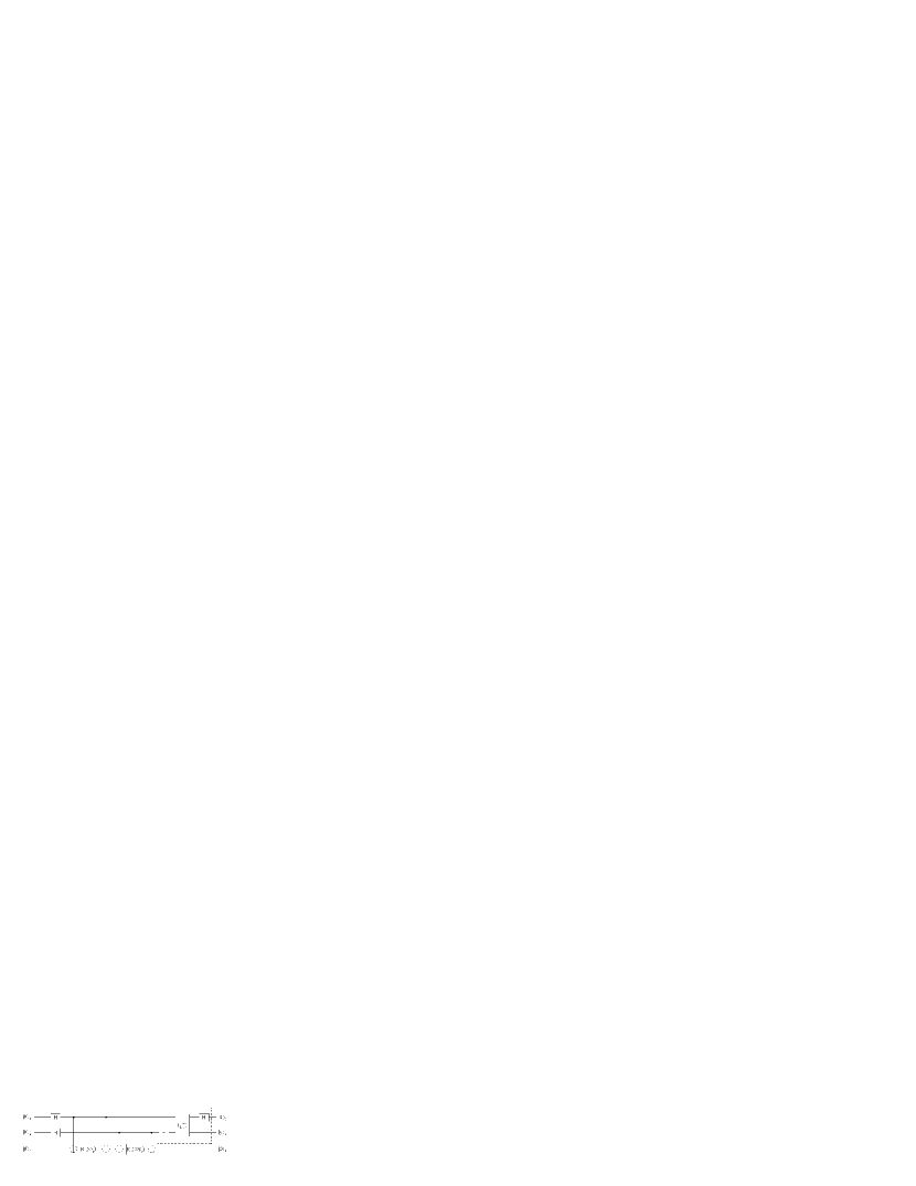
Figure 1: The quantum network to implement the QCS algorithm. The three lines denote the three qubits. $H$ denotes the Hadmamard transform, $I_{|11\rangle}^{-\pi/2}$ denotes the controlled phase shift operation, and $R_{z}(\varphi_{k})=e^{i\varphi_{k}I_{z}}$, where $\varphi_{k}=-k\pi/2$ $(k=0,1,2,3)$. The network outlined by the dashed rectangle implements the inverse of quantum Fourier transform without the SWAP operation. Time goes from left to right. $|x\rangle_{1}|y\rangle_{2}$ is the output state, which can be obtained through measuring qubits 1 and 2.

Figure 2: Pulse sequence to realize $[\tau]_{13}$ (a) and the chemical shift evolution $R^{2}_{z}(2\pi\delta 8t)$ (b), where $\delta$ is the offset between the chemical shift of C2 and the transmitter frequency. Rectangles denote $\pi$ pulses. The narrow ones are so short that the widths can be ignored. The wide ones, however, are long pulses of which widths can not be ignored.

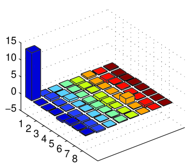
Figure 3: The density matrix (in arbitrary units) reconstructed using the state tomography technique, when the system is prepared in effective- pure state $|000\rangle$.

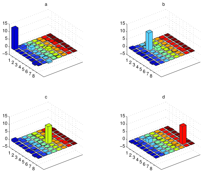
Figure 4: The density matrices of the three- qubit system, after the implementation of the QCS algorithm. Only the real components are plotted. The imaginary portions, which are theoretically zero, are found to contribute less than $10\%$ to the experimental results. Figs. (a-d) correspond to the four effective- pure states $|000\rangle$, $|010\rangle$, $|100\rangle$, and $|110\rangle$, and the four effective- pure states correspond to the four different time differences $\Delta=0$, $\Delta=1/4\omega$, $\Delta=1/2\omega$, and $\Delta=3/4\omega$, respectively.

References

- (1) P. W. Shor, Proc. 35th Annual IEEE Symposium on Foundations of Computer Science-FOCS, 20-22 (1994)
- (2) I. L. Chuang, Phys. Rev. Lett, 85, 2006(2000)
- (3) R. Jozsa, D. S. Abrams, J. P. Dowling, and C. P. Williams, Phys. Rev. Lett, 85, 2010(2000)
- (4) V. Giovannetti, S. Lloyd, and L. Maccone, Narure, 412, 417(2001)
- (5) A. Y. Kitaev, quantum measurements and the Abelian stabilizer problem, arXiv eprint quant-ph/9511026, 1995.
- (6) R. Cleve, A. Ekert, C. Macchiavello, and M. Mosca, P. R. Soc. London A, 454 (1969): 339, 1998.
- (7) I. L. Chuang, N. Gershenfeld, and M. Kubinec. Phys. Rev. Lett. 80, 3408 (1998)
- (8) L. M. K. Vandersypen, M. Steffen, G. Breyta, C. S. Yannoni, M. H. Sherwood, and I. L. Chuang, Nature, 414, 883(2001)
- (9) Y. S. Weinstein, M. A. Pravia, E. M. Fortunato, S. Lloyd, and D. G. Cory, Phys. Rev. Lett, 86, 1889(2001)
- (10) G. L. Long, L. Xiao, J. Chem. Phys. 119, 8473-8481 (2003)
- (11) X.-H. Peng, X.-W. Zhu, M. Fang, M.-L. Liu, K.-L. Gao, Phys. Rev. A65 042315 (2002)
- (12) M.A. Nielsen, E. Knill and R. Laflamme, Nature 396, 52(1998)
- (13) X. M. Fang, X.- W. Zhu , M. Feng , X.- A. Mao, and F. Du, Phys. Rev. A, 61, 022307(2000)
- (14) D. X. Wei et al, Chinese Science Bulletin, 48, 2501 (2003)
- (15) L. M. K. Vandersypen, M. Steffen, G. Breyta, C. S. Yannoni, R. Cleve, and I. L. Chuang, Phys. Rev. Lett, 85, 5452 (2000)
- (16) Y. S. Weinstein, S. Lloyd, J. Emerson and D. G. Cory, Phys. Rev. Lett, 89, 157902 (2002)
- (17) D. G. Cory, A. F. Fahmy, and T. F. Havel, PNAS 94, 1634(1997).
- (18) N. A. Gershenfeld and I. L.Chuang, Science 275, 350 (1997).
- (19) I. L. Chuang, N. Gershenfeld, M. G. Kubinec and D. W. Leung, Proc. R. Soc. Lond. A 454,447 (1998)
- (20) D. G. Cory, M. D. Price, and T. F. Havel, Physica D.120,82 (1998)
- (21) E. Knill, I. Chuang, and R. Laflamme, Phys. Rev. A, 57, 3348(1998)
- (22) S. Somaroo, C. H. Tseng, T. F. Havel, R. Laflamme, and D. G. Cory Phys. Rev. Lett, 82, 5381(1999)
- (23) E. Knill, R. Laflamme, R. Martinez, and C.-H. Tseng, Nature, 404, 368(2000)
- (24) D. G. Cory, M. D. Price, W. Maas, E. Knill, R. Laflamme, W. H. Zurek, T. F. Havel, and S. S. Somaroo, Phys. Rev. Lett, 81, 2152(1998)
- (25) N. Boulant, E. M. Fortunato, M. A. Pravia, G. Teklemariam, D. G. Cory, and T. F. Havel, Phys. Rev. A 65, 024302 (2002)
- (26) G. Teklemariam, E. M. Fortunato, M. A. Pravia, Y. Sharf, T. F. Have D. G. Cory, A. Bhattaharyya, and J. Hou, Phys. Rev. A 66, 012309 (2002)
- (27) N. Boulant, K. Edmonds, J. Yang, M. A. Pravia, and D. G. Cory, Phys. Rev. A 68, 032305 (2003)
- (28) L. Viola, E. M. Fortunato, M. A. Pravia, E. Knill,1 R. Laflamme, David G. Cory, Science, 293, 2059(2001)
- (29) R. R. Ernst, G. Bodenhausen and A. Wokaum, Principles of nuclear magnegtic resonance in one and two dimensions, Oxford University Press(1987)
- (30) N.Linden, . Kupe, and R. Freeman, Chem. Phys. Lett, 311, 321(1999)
- (31) N. Linden, B. Herv, R. J. Carbajo, and R. Freeman, Chem. Phys. Lett, 305, 28(1999)
- (32) H. Geen, and R. Freeman, J. Magn. Reson. 93, 93 (1991)
- (33) J.-F Zhang, Z.-H Lu, L. Shan, and Z.-W. Deng, Phys. Rev. A, 66, 044308(2002).
- (34) G. L. Long et al, Phys. Lett. A 286, 121 (2001)
- (35) L. M. K. Vandersypen, and I. L. Chuang, arXiv eprint quant-ph/0404064
- (36) G. M. Leskowitz, and L. J. Mueller, Phys. Rev. A 69, 052302 (2004)
- (37) L. M. K. Vandersypen, M. Steffen, M. H. Sherwood, C. S. Yannoni, G. Breyta, and I. L. Chuang, Appl. Phys. Lett, 76, 646(2000)