Modularization of the multi-qubit controlled phase gate and its NMR implementation

Abstract

Quantum circuit network is a set of circuits that implements a certain computation task. Being at the center of the quantum circuit network, the multi-qubit controlled phase shift is one of the most important quantum gates. In this paper, we apply the method of modular structuring in classical computer architecture to quantum computer and give a recursive realization of the multi-qubit phase gate. This realization of the controlled phase shift gate is convenient in realizing certain quantum algorithms. We have experimentally implemented this modularized multi-qubit controlled phase gate in a three qubit nuclear magnetic resonance (NMR) quantum system. The network is demonstrated experimentally using line selective pulses in NMR technique. The procedure has the advantage of being simple and easy to implement.

I Introduction

Quantum computer is born with the combination of quantum mechanics and computer science. Quantum properties have enabled quantum computer to outperform a classical computer for factorizing a large number shor , or searching an unordered database Grover97 . In Ref. Deutsch85 , Deutsch proposed quantum gates and quantum network, and described a blue print for quantum computer. It has been shown that it is possible to construct arbitrary $n$-qubit quantum gate by using only a finite set of one-qubit gates and two-qubit gates Deutsch95 ; Bremner . These basic quantum gates are universal for quantum computationNielsen . Barenco et al, and Cleve have developed methods for designing networks in multiple- qubit system Barenco ; Cleve .

Quantum network can be viewed as the quantum analog of the classical computing. It provides with us a convenient method to build a quantum computer similar to building a classical computer. A classical compute can be implemented as a fixed classical gate array, with an input programm and data. A universal gate array can be programmed to perform any possible function on the input data. However for a quantum computer, Nielsen and Chuang demonstrated a rather different property Nielsen97 . They pointed out it is not possible to build a fixed, general purpose quantum computer which can be programmed to perform any arbitrary quantum computation task. The implementation of a universal quantum gate array on a quantum computer can only be realized in a probabilistic fashion, not in a deterministic fashion. By extending the one-to-one processor to one-input-to multiple-output processor, Yu et al proposed an approximate and probabilistic programmable multi-output quantum processor Yu . Schuch et al proposed a general programmable network to implement arbitrary two-qubit phase-shift operation with a network of one-qubit and two- qubit operations Schuch . It embodies the following transformation $|x\rangle\rightarrow e^{-i\theta_{x}}|x\rangle$ where $x$ runs over all possible basis states. Other interesting results were also obtained Vidal ; Rosko ; Pable ; Barenco ; Vandersypen .

In quantum computation, a special controlled phase gate is of particular importance: it only changes the phase for a particular basis state $|s\rangle$, and leaves the other basis states unchanged. For instance, in the Grover quantum search algorithmGrover97 , there are two phase inversions, $I_{\tau}$ which inverses the phase of the marked state and leaves alone the phases of other basis states, and $I_{0}$ which acts likewise. Starting from this controlled phase gate, other controlled gate operation, such as the multi-qubit controlled-not gate can be realized, and multi-qubit controlled gate is the major operation in many practical application such as initializing a quantum computer from $|00\cdots 0\rangle$ into an arbitrary superposed statelongsun , and in designing quantum cloning machinesknight . This multi-qubit gate can be decomposed into a set of one-qubit gate and two-qubit gates as given in Ref.Barenco . In fact, this decomposition has been used in, for instance, Refs.jcplong ; Du to implement multi-qubit controlled-NOT gate. In the same spirit, the multi-qubit controlled phase gate can be implemented systematically using the method proposed in Ref. Schuch .

In this paper, we propose a different realization scheme for the $n$ -qubit controlled phase gate using modular structure and recursion. The network retains the same form when the system extends to more qubits. It contains an $n$-qubit controlled phase rotation about the $z$-axis plus an $n-1$- qubit controlled phase gate. Again the $n-1$- qubit controlled phase gate can then be further realized similarly. In one hand, the controlled phase gate is used in many computing algorithms, and it merits special attention. In the other hand, the modular realization of this controlled phase gate may provide convenience for some physical systems such as the nuclear magnetic resonance(NMR). Das et al proposed the scheme to implement the controlled phase-shift gate in the NMR system using line-selective pulses, where a controlled phase rotation was realized through three line selective pulses Das . A line-selective pulse is the high-selective radio-frequency pulse designed to perturbed transverse magnetization one line at a time Linden98 . Experimentally, line-selective pulses can simplify a network circuit greatly, and makes it easy to extend the circuit to more qubits. The operational time of a line-selective pulse is not influenced by the number of the qubits but the spin system with well resolved couplings Du . For some certain systems, the line-selective pulses can use short time and this is an attractive feature considering the limited decoherence time in candidate quantum computer realization systems. Das et al demonstrated their scheme in a three qubit NMR system by simulations and in a two qubit system experimentally. Their method can be applicable for both the weakly-coupled spin systems and the strongly coupled systems.

Our work concentrates on the weakly-coupled spin systems, which have been widely used in quantum computation Chuang . We have experimentally demonstrated the feasibility of the proposed network in a three qubit NMR quantum system, where the multi-qubit controlled phase rotation is realized by the line-selective radio-frequency pulses and the spin selective pulses on the target qubit. Compared with the method used in Das et al’s work, our method is experimentally simple. In our experiment, the line-selective pulse that pin-points directly the right frequency for the controlled configuration has been successfully demonstrated. The line-selective pulse has the advantage of the reduced operating time and ease in algorithm design.

The paper is organized as follows. In section II, we describe the modularized realization of the multi-qubit controlled phase gate. In section III, we report the details of the experimental realization in a three-qubit NMR quantum system. In section IV, we discuss some issues in the realization and a briefly summarize the result.

II Modularized quantum network for controlled phase gate

The controlled phase- shift gate is one of most important operation in quantum computation. On one hand, with a two-bit phase gate and one-qubit rotation gate, one can build any arbitrary unitary operation in quantum computation. On the other hand, multi-qubit controlled phase gate is the essential operation in many quantum algorithms, such as the Grover quantum search algorithm, quantum Fourier transform and so onGrover97 ; Grover98 ; Biham ; Weinstein . The controlled phase- shift operation for $n$-qubit system is denoted by $I_{|s_{n}\rangle}^{\varphi}$, where $|s_{n}\rangle$ is a basis state of an $n$-qubit system. $I_{|s_{n}\rangle}^{\varphi}$ transforms $|s_{n}\rangle$ to $e^{i\varphi}|s_{n}\rangle$, and leaves the other basis states unaltered. Without loss of generality, we assume that qubit $n$ is the target bit, and the other $n-1$ qubits are the controlling bits. Let $|s_{n}\rangle=|1\cdots 1\rangle$, denoting that all qubits lie in state $|1\rangle$. $I_{|s_{n}\rangle}^{\varphi}$ can be expressed as

$$I_{|s_{n}\rangle}^{\varphi}=\left(\begin{array}[]{cc}I_{2^{n}-2}&0\\ 0&U\\ \end{array}\right),$$ (1)

where

$$U=\left(\begin{array}[]{cc}1&0\\ 0&e^{i\varphi}\\ \end{array}\right),$$ (2)

and $I_{2^{n}-2}$ denotes the $(2^{n}-2)\times(2^{n}-2)$ unit matrix. $U$ is an operation applied to the target qubit. $U$ cannot be constructed from the Pauli operators $\sigma_{x}$, $\sigma_{y}$, $\sigma_{z}$ and $I_{2}$ directly, because it is not in $SU(2)$ groupBarenco . Practically, $U$ can be realized in the following manner, noting that

$$U=\left(\begin{array}[]{cc}e^{i\varphi/2}&0\\ 0&e^{i\varphi/2}\end{array}\right)\left(\begin{array}[]{cc}e^{-i\varphi/2}&0\\ 0&e^{i\varphi/2}\\ \end{array}\right)\equiv\Phi(\varphi/2)R_{z}(-\varphi),$$ (3)

where $R_{z}(-\varphi)\equiv e^{-i\varphi I_{z}}$. $I_{z}$ is $\hat{z}$-component of the angular momentum of the spin, and $I_{z}|0\rangle={1\over 2}|0\rangle$, $I_{z}|1\rangle=-{1\over 2}|1\rangle$, by setting $\hbar=1$. $R_{z}(-\varphi)$ can be realized by a rotation about the $z$-axis, and in NMR it is realized by radio-frequency (rf) pulsesLinden . For a single qubit, the difference between $R_{z}(-\varphi)$ and $U$ is negligible because they differ only by a global phase. But for the controlled phase gate, this difference cannot be ignored. For instance, in a two-qubit system, the controlled-rotation $R^{C}_{z}(\varphi)$ is

$$R^{C}_{z}(\varphi)=\left({\begin{array}[]{cccc}1&0&0&0\\ 0&1&0&0\\ 0&0&e^{-i\varphi/2}&0\\ 0&0&0&e^{i\varphi/2}\end{array}}\right),$$ (8)

and it is obvious the overall phase between $U$ and $R_{z}$ is no longer trivial, and $\Phi(\varphi/2)$ must be considered in designing the network for $I_{|s_{n}\rangle}^{\varphi}$.

The network to implement $I_{|s_{n}\rangle}^{\varphi}$ is shown by Fig. 1, where the ”global” controlled-$\Phi(\varphi/2)$ is explicitly drawn. By a simple observation, it is not difficult to show that the controlled-$\Phi(\varphi/2)$ is equivalent to:

$$\Phi^{C\cdots C}(\varphi/2)=I_{|s_{n-1}\rangle}^{\varphi/2},$$ (9)

where $I_{|s_{n-1}\rangle}^{\varphi/2}$ denotes the phase- shift operation for the $n-1$- qubit system composed of the control qubits in the original $n$-qubit system. $|s_{n-1}\rangle$ is the basis state of the first $n-1$ control qubits where the corresponding basis state of the whole $n$ qubit is $|s_{n}\rangle=|s_{n-1}\rangle|1\rangle_{n}$. The $n-1$-th qubit is the target qubit, the other $n-2$ qubits are the control qubits in $I_{|s_{n-1}\rangle}^{\varphi/2}$. The effect of this shortened controlled phase gate can be seen as follows: the controlled-phase rotation $R^{C}_{z}(\varphi)$ changes

$$|s_{n-1}0\rangle \rightarrow e^{-i\varphi/2}|s_{n-1}0\rangle,$$

$$|s_{n-1}1\rangle \rightarrow e^{i\varphi/2}|s_{n-1}1\rangle,$$ (10)

and it leaves other basis states unaltered. A follow-up $I_{|s_{n-1}\rangle}^{\varphi/2}$ operation changes $|s_{n-1}\rangle$ into $e^{i\varphi/2}|s_{n-1}\rangle$, and this takes $e^{-i\varphi/2}|s_{n-1}0\rangle$ into $|s_{n-1}0\rangle$, and $e^{i\varphi/2}|s_{n-1}1\rangle$ into $e^{i\varphi}|s_{n-1}1\rangle$. Hence the total effect is to change $|s_{n}\rangle$ into $e^{i\varphi}|s_{n}\rangle$. Fig. 1 can be further represented as Fig. 2, where $I_{|s_{n-1}\rangle}^{\varphi/2}$ is applied to the control qubits. We call the $I_{|s_{n-1}\rangle}^{\varphi/2}$ part as the compensatory network module. The controlled-phase rotation can be realized by two multi-qubit controlled-NOT gates ($\Lambda_{n-1}({\rm NOT})$) and two single-bit phase rotations Barenco . $\Lambda_{n-1}({\rm NOT})$ can be directly realized in some physical realizations such as the NMR system, or be further reduced to a set of single qubit rotations and two-qubit controlled NOT gates as described in Ref.Barenco .

The nice feature in Fig.2 is that $I_{|s_{n-1}\rangle}^{\varphi/2}$ can be realized in the same way as $I_{|s_{n}\rangle}^{\varphi}$: it can be realized by a compensatory module composed of the $n-2$ qubits together with an $n-2$ qubits controlled phase rotation, and the compensatory module unit can be similarly constructed shown as the right network in Fig. 2. Hence we have obtained a recursive way to construct the multi-qubit phase shift gate. In summary, $I_{|s_{n}\rangle}^{\varphi}$ is constructed by the n-1 -qubit controlled phase rotation and the compensatory network module $I_{|s_{n-1}\rangle}^{\varphi/2}$. $I_{|s_{n}\rangle}^{\varphi}$ is realized recursively.

III NMR realization of the modularized network

In the experiment, we use a sample of Carbon-13 labelled trichloroethylene (TCE) dissolved in d-chloroform. Data are taken at controlled temperature (22⁰) with a Bruker DRX 500 MHz spectrometer. ¹H is denoted as qubit 3, the ¹³C directly connecting to ¹H is denoted as qubit 2, and the other ¹³C is denoted as qubit 1. The three qubits are denoted as C1, C2 and H3. By setting $\hbar=1$, the Hamitonian of the three-qubit system is

$$H=-2\pi\nu_{1}I_{z}^{1}-2\pi\nu_{2}I_{z}^{2}-2\pi\nu_{3}I_{z}^{3}+2\pi J_{12}I_{z}^{1}I_{z}^{2}+2\pi J_{23}I_{z}^{2}I_{z}^{3}+2\pi J_{13}I_{z}^{1}I_{z}^{3},$$ (11)

where $\nu_{1}$, $\nu_{2}$, $\nu_{3}$ are the resonance frequencies for C1, C2 and H3, respectively, and $\nu_{1}=\nu_{2}+904.4$Hz. The coupling constants are measured to be $J_{12}=103.1$ Hz, $J_{23}=203.8$ Hz, and $J_{13}=9.16$ Hz respectively.

We realize $I_{|11\rangle}^{\varphi}$ in the two-qubit system composed of C1 and C2, through decoupling H3. The spin-coupling evolution between C1 and C2 is described by

$$[\tau]=e^{-i2\pi J\tau I_{z}^{1}I_{z}^{2}}.$$ (12)

C1 and C2 construct a homonuclear system, which can demonstrate the implementation of $I_{|11\rangle}^{\varphi}$ clearly, and represent the effect of the compensatory module. Fig. 2 is simplified to a two-qubit network, where C1 is the control qubit, and C2 is the target qubit. The compensatory module is expressed as $I_{|1\rangle}^{\varphi/2}=\Phi^{1}(\varphi/4)R_{z}^{1}(-\varphi/2)$, and is equivalent to $R_{z}^{1}(-\varphi/2)$. $\Phi^{1}(\varphi/4)$ only contributes an irrelevant overall phase factor before $I_{|11\rangle}^{\varphi}$. $\Lambda_{n-1}(NOT)$ is the ordinary CNOT operation. The operation sequence CNOT-$R_{z}^{2}(\varphi/2)$-CNOT can be realized by $[\frac{-\varphi}{2\pi J_{12}}]$. Hence $I_{|11\rangle}^{\varphi}$ is realized by the following pulse sequence

$$R_{z}^{1,2}(-\varphi/2)-[\frac{-\varphi}{2\pi J_{12}}],$$

where $\varphi$ is taken as the menus value during the experiment.

The experiment starts with the pseudo-pure state prepared by spatial averaging. The following pulse sequence Somarooprl991 ; Fang

$$[\frac{\pi}{4}]_{x}^{1,2}-\frac{1}{4J_{12}}-[\pi]_{y}^{1,2}-\frac{1}{4J_{12}}-[-\pi]_{y}^{1,2}-[-\frac{5\pi}{6}]_{y}^{1,2}-[grad]_{z}$$

transforms the system from equilibrium state to the pseudo-pure state

$$\rho_{ini}=I_{z}^{1}/2+I_{z}^{2}/2+I_{z}^{1}I_{z}^{2},$$ (13)

which is equivalent to state $|00\rangle$. The symbol $1/4J_{12}$ denotes the evolution caused by the magnetic field for $1/4J_{12}$ when the pulses are switched off. After the application of the Hadamard transform, $|00\rangle$ is transform to the superposition of states

$$|p\rangle=(|00\rangle+|01\rangle+|10\rangle+|11\rangle)/2.$$ (14)

It is obvious $I_{|11\rangle}^{\varphi}|p\rangle=(|00\rangle+|01\rangle+|10\rangle+e^{i\varphi}|11\rangle)/2$, represented by density matrix

$$\rho_{f}=\frac{1}{4}\left(\begin{array}[]{cccc}1&1&1&e^{-i\varphi}\\ 1&1&1&e^{-i\varphi}\\ 1&1&1&e^{-i\varphi}\\ e^{i\varphi}&e^{i\varphi}&e^{i\varphi}&1\\ \end{array}\right).$$ (15)

In Eq. (15), the matrix elements $\rho_{f}(1,3)$ and $\rho_{f}(2,4)$ can be directly observed through the spectra of C1, and $\rho_{f}(1,2)$, $\rho_{f}(3,4)$ can be directly observed through the spectra of C2.

The Hadamard transform is realized by $[-\frac{\pi}{2}]_{y}^{1,2}-[\pi]_{x}^{1,2}$. $I_{|11\rangle}^{\varphi}$ is realized by

$$\frac{-\varphi}{4\pi J_{12}}-[\pi]_{y}^{1,2}-\frac{-\varphi}{4\pi J_{12}}-[-\pi]_{y}^{1,2}-[-\frac{\pi}{2}]_{y}^{1,2}-[-\frac{\varphi}{2}]_{x}^{1,2}-[\frac{\pi}{2}]_{y}^{1,2}.$$

Figs. 3(a-d) show the results when $-\varphi/2=\pi/4$, $\pi/2$, $3\pi/4$ and $\pi$, respectively. In each figure, the frequency centers of the doublets of C1 and C2 are 124.14ppm and 116.91ppm, respectively. The right and left peaks in the doublet of C1 correspond to $\rho_{f}(1,3)$ and $\rho_{f}(2,4)$ in Eq.(15), and the right and left ones in the doublet of of C2 correspond to $\rho_{f}(1,2)$ and $\rho_{f}(3,4)$ in Eq.(15) respectively. The phases of the right peaks of C1 and C2 hardly change with $-\varphi/2$. They are chosen as the reference phases to observe the phases of the other peaks so that the phases of signals are meaningfulJones . The phase of the left peak (denoted by $Ph2$) changes via $-\varphi/2$ proportionably, which are shown in Fig. 4.

To show the effect of the compensatory module, we add $R^{1}_{z}(\varphi/2)$ at the end of network shown in Fig. 2 to cancel the compensatory network module. The network without the compensatory network module implements the transformation

$$I_{|11\rangle}^{\varphi}R^{1}_{z}(\varphi/2)=e^{i\varphi/4}\left(\begin{array}[]{cccc}1&0&0&0\\ 0&1&0&0\\ 0&0&e^{-i\varphi/2}&0\\ 0&0&0&e^{i\varphi/2}\\ \end{array}\right).$$ (16)

It is obvious that $I_{|11\rangle}^{\varphi}R^{1}_{z}(\varphi/2)|p\rangle=e^{i\varphi/4}(|00\rangle+|01\rangle+e^{-i\varphi/2}|10\rangle+e^{i\varphi/2}|11\rangle)/2$, which is represented as

$$\rho_{f}^{{}^{\prime}}=\frac{1}{4}\left(\begin{array}[]{cccc}1&1&e^{i\varphi/2}&e^{-i\varphi/2}\\ 1&1&e^{i\varphi/2}&e^{-i\varphi/2}\\ e^{-i\varphi/2}&e^{-i\varphi/2}&1&e^{-i\varphi}\\ e^{i\varphi/2}&e^{i\varphi/2}&e^{i\varphi}&1\\ \end{array}\right).$$ (17)

From Eq. (17), the signals of C1 and C2 have phase difference, which can be observed in this homonuclear system.

$R^{1}_{z}(\varphi/2)$ can be realized by

$$t-[\pi]_{y}^{2}-2t-[-\pi]_{y}^{2}-t.$$

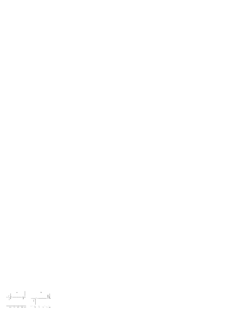
Figure 5: ${}^{13}C$ spectra after $I_{|11\rangle}^{\varphi}R^{1}_{z}(\varphi/2)$ is applying to the uniform superposition of basis states, when $-\varphi/2=\pi/2$, $\pi$, shown by Figs. (a) and (b), respectively.

In theory, $\varphi/2=4(\nu_{1}-\nu_{2})2\pi(t+t_{p}/2)$, where $t_{p}$ is the width of the $\pi$ pulse selective for C2 Linden . However, the dependence of $\varphi/2$ on $t$ needs be measured due to the errors caused by decoherence and imperfection in the pulses. Figs. 5(a-b) show the results of $I_{|11\rangle}^{\varphi}R^{1}_{z}(\varphi/2)|p\rangle$ with $-\varphi/2=\pi/2$, $\pi$. Compared with Figs. 4(b) and (d), consequently the phases in peaks C1 and C2 are no longer the same. Theoretically this phase difference should be $\varphi/2$, and our experiment results agree with this theoretical expectation.

IV Discussion and summary

We realize the network shown in Fig. 6 in a three qubit system by switching off the decoupling pulses for $H3$. The network consists of two rotation operations for C2 and two controlled-controlled-NOT gates (CCNOT or Toffoli gate). C2 is the target qubit, C1 and H3 are the control qubits with control condition $|0\rangle_{1}|1\rangle_{3}$. The network implements the transform $I^{-\varphi/2}_{|001\rangle}I^{\varphi/2}_{|011\rangle}$, which can be transformed to $I^{\varphi}_{|011\rangle}$ by multiplying $I^{\varphi/2}_{|001\rangle}I^{\varphi/2}_{|011\rangle}$. In fact, $I^{\varphi/2}_{|001\rangle}I^{\varphi/2}_{|011\rangle}$ is the controlled phase- shift operation for the system composed of C1 and H3, and it is represented as

$$I_{|0\rangle_{1}|1\rangle_{3}}^{\varphi/2}=\left(\begin{array}[]{cccc}1&0&0&0\\ 0&e^{i\varphi/2}&0&0\\ 0&0&1&0\\ 0&0&0&1\end{array}\right),$$ (18)

with the basis state order $|0\rangle_{1}|0\rangle_{3}$, $|0\rangle_{1}|1\rangle_{3}$, $|1\rangle_{1}|0\rangle_{3}$, $|1\rangle_{1}|1\rangle_{3}$. $I_{|0\rangle_{1}|1\rangle_{3}}^{\varphi/2}$ can realized by a similar way in Sec. III. $I^{-\varphi/2}_{|001\rangle}I^{\varphi/2}_{|011\rangle}$ transforms the superposition of states

$$|p\rangle_{3}=(|000\rangle-|001\rangle-|010\rangle+|011\rangle)/2$$ (19)

to $(|000\rangle-e^{-i\varphi/2}|001\rangle-|010\rangle+e^{i\varphi/2}|011\rangle)/2$, expressed as the density matrix

$$\rho_{f3}=\left(\begin{array}[]{cccccccc}1&-e^{i\varphi/2}&-1&e^{-i\varphi/2}&0&0&0&0\\ -e^{-i\varphi/2}&1&e^{-i\varphi/2}&-e^{-i\varphi}&0&0&0&0\\ -1&e^{i\varphi/2}&1&-e^{-i\varphi/2}&0&0&0&0\\ e^{i\varphi/2}&-e^{i\varphi}&-e^{i\varphi/2}&1&0&0&0&0\\ 0&0&0&0&0&0&0&0\\ 0&0&0&0&0&0&0&0\\ 0&0&0&0&0&0&0&0\\ 0&0&0&0&0&0&0&0\\ \end{array}\right),$$ (20)

where $|p\rangle_{3}$ is obtained by applying $[\frac{\pi}{2}]_{y}^{2,3}$ to $|000\rangle$. The elements (1,3) and (2,4) in the matrix can be observed in the spectrum of C2 directly.

The pseudo-pure state $|000\rangle$ can be represented by

$$\rho_{eff}=(\frac{1}{2}I+I_{z}^{1})(\frac{1}{2}I+I_{z}^{2})(\frac{1}{2}I+I_{z}^{3}).$$ (21)

$\rho_{eff}$ can be expressed as $\rho_{eff}\equiv\rho_{1}+\rho_{2}+\frac{1}{8}I_{8\times 8}$, where

$$\rho_{1}=(\frac{1}{2}I_{z}^{1}+\frac{1}{2}I_{z}^{2}+I_{z}^{1}I_{z}^{2}+\frac{1}{4})I_{z}^{3},$$ (22)

$$\rho_{2}=\frac{1}{2}(\frac{1}{2}I_{z}^{1}+\frac{1}{2}I_{z}^{2}+I_{z}^{1}I_{z}^{2}),$$ (23)

and the last term $\frac{1}{8}I_{8\times 8}$ can be ignored Knill1 . Quantum computation can start with $\rho_{1}$ and $\rho_{2}$, respectively. The average of the two results is equivalent to the result obtained from the initial state $\rho_{eff}$. Because the results of applying $[\frac{\pi}{2}]_{y}^{2,3}$ to $\rho_{1}$ have no observable signals in the carbon spectra, it is sufficient to use $\rho_{2}$ as the initial state to observe the results of applying $I^{-\varphi/2}_{|001\rangle}I^{\varphi/2}_{|011\rangle}$ to $|p\rangle_{3}$. This fact can simplify the process of experiments greatly.

The initial state described as Eq. (23) is realized by $[\frac{\pi}{2}]_{y}^{3}-[grad]_{z}-[\frac{\pi}{4}]_{x}^{1,2}-\frac{1}{8J_{12}}-[\pi]_{y}^{3}-\frac{1}{8J_{12}}-[\pi]_{y}^{1,2,3}-\frac{1}{8J_{12}}-[-\pi]_{y}^{3}-\frac{1}{8J_{12}}-[-\pi]_{y}^{1,2,3}-[-\frac{5\pi}{6}]_{y}^{1,2}-[grad]_{z}$. CCNOT gate can be approximately realized by a line selective $\pi$ pulse with frequency $\nu_{2}+J_{12}/2-J_{23}/2$, which causes transition $|001\rangle\leftrightarrow|011\rangle$. Figs. 7 show the results of $I^{-\varphi/2}_{|001\rangle}I^{\varphi/2}_{|011\rangle}$$|p\rangle_{3}$. In each figure, the right peak, with frequency $\nu_{2}+J_{12}/2+J_{23}/2$, corresponds the element (1,3), and the left peak, with frequency $\nu_{2}+J_{12}/2-J_{23}/2$, corresponds the element (2,4), which changes versus $\varphi/2$. Figs. 7 (a-f) show the results of $\varphi/2=0$, $25.2^{\circ}$, $38.2^{\circ}$, $90^{\circ}$, $141.8^{\circ}$, $154.7^{\circ}$, respectively. The graph in Fig. 8 shows the phase of the right peak (denoted by $Ph3$) versus $\varphi/2$. It can be fitted as a line with slope approximate to 1.95. In theory, slope is -2. The difference of sign results from the approximation of CCNOT gates.

The modularized quantum network to implement the controlled phase- shift gate is proposed, and realized on a three qubit NMR quantum computer. The $n$- qubit network nests the $n-1$- qubit network. This idea represents the essential thoughts of computer science. The quantum modules provide a systemic method to building practical quantum computers. It is sure that the modularized quantum networks will play central role for large- scale quantum computer.

Figure 1: The quantum network to implement $I_{|s_{n}\rangle}^{\varphi}$. The lines represent the $n$ qubits, respectively. Qubit $n$ is the target qubit, and the other qubits are the control ones. $\Phi(\varphi/2)$ is a phase- shift operation, and $R_{z}(-\varphi)=e^{-i\varphi I_{z}}$.

Figure 2: The network in Fig. 1 which is represented by a multiple qubit-controlled phase rotation operation and a compensatory network module, denoted by $I_{|s_{n-1}\rangle}^{\varphi/2}$, which is equivalent to the multiple qubit-controlled $\Phi(\varphi/2)$ in Fig. 1. The compensatory network module can be further decomposed as the network circuit denoted by the dashed rectangle in the right network.

Figure 3: ${}^{13}C$ spectra of trichloroethylene after $I_{|s_{n}\rangle}^{\varphi}$ is applied to the uniform superposition of basis states obtained through applying Hadmamard transform to $|00\rangle$. ${}^{1}H$ has been decoupled. The phases of the right peaks of in the doublets hardly change. The phases of the left peaks, denoted by $Ph2$ (2 for the two qubit system), change with $-\varphi/2$ proportionably. Figs. (a-d) are the spectra for $-\varphi/2=\pi/4$, $\pi/2$, $3\pi/4$ and $\pi$, respectively.

Figure 4: The phase of the left peak in the doublet of C1 or C2, which is denoted as $Ph2$, versus $-\varphi/2$. The graph can be fitted as a line with slope equal to 1.96. The theoretical expectation is 2.

Figure 6: The quantum network to implement $I^{-\varphi/2}_{|001\rangle}I^{\varphi/2}_{|011\rangle}$.

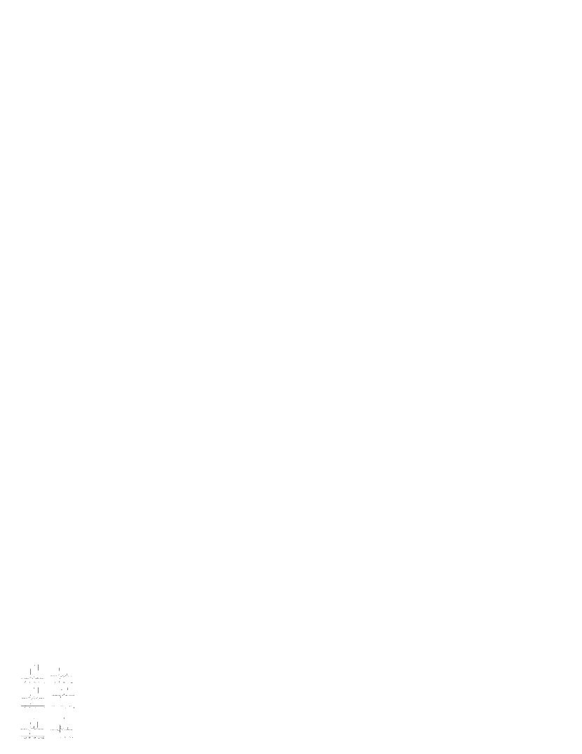
Figure 7: Spectra of C2 after $I^{-\varphi/2}_{|001\rangle}I^{\varphi/2}_{|011\rangle}$ is applied to $(|000\rangle-|001\rangle-|010\rangle+|011\rangle)/2$. Only two NMR peaks appear in each spectrum. The phase of the right peak hardly changes. The phase of the left peak changes with $\varphi/2$, proportionably. Figs. (a-f) show the spectra for $\varphi/2=0$, $25.2^{\circ}$, $38.2^{\circ}$, $90^{\circ}$, $141.8^{\circ}$, $154.7^{\circ}$, respectively.

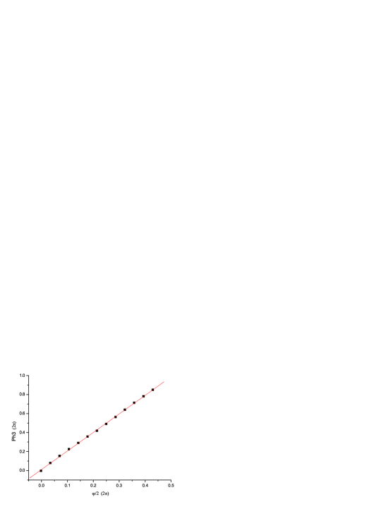
Figure 8: The phase of the left peak in the spectrum shown in Fig. 7, which is denoted as $Ph3$, versus $\varphi/2$. The graph can be fitted as a line with slope approximate to 1.95. In theory, slope is -2. The difference of sign results from the approximation of CCNOT gates.

References

- (1) P W Shor, Proc. 35th Annual IEEE Symposium on Foundations of Computer Science-FOCS, 20-22 (1994)
- (2) L. K. Grover, Phys. Rev. Lett. 79, 325 (1997)
- (3) D. Deutsch, Proc. R. Soc. A, 400, 97-117(1985)
- (4) D. Deutsch, A. Barenco, and A. Ekert, Proc. R. Soc. London A 449, 669 (1995); quant-ph/9505018
- (5) M. J. Bremner, C. M. Dawson, J. L. Dodd, A. Gilchrist, A. W. Harrow, D. Mortimer, M. A. Nielsen, and T. J. Osborne1, Phys. Rev. Lett, 89, 247902 (2002)
- (6) M. A. Nielsen, and I. L. Chuang, Quantum computation and quantum information(Cambridge University Press,2000)
- (7) A. Barenco, C. H. Bennett, R. Cleve, D. P. DiVincenzo, N. Margolus, P. Shor, T. Sleator, J. A. Smolin, and H. Weinfurter, Phys. Rev. A, 52, 3457(1995)
- (8) R. Cleve, A. Ekert, C. Macchiavello, and M. Mosca, Proc. R. Soc, Lond, A 454, 339 (1998)
- (9) M. A. Nielsen, and I. L. Chuang, Phys. Rev. Lett. 79, 321 (1997)
- (10) Y.-F. Yu, J. Feng, and M. -S. Zhan, Phys. Rev. A 66, 052310 (2002)
- (11) N. Schunch, and J. Siewert, Phys. Rev. Lett, 91, 027902(2003)
- (12) G. Vidal, L. Masanes, and J. I. Cirac, Phys. Rev. Lett. 88, 047905 (2002)
- (13) M. Roko, V. Buek, P. R. Chouha, and M. Hillery, Phys. Rev. A 68, 062302 (2003)
- (14) J. P. Paz, and A. Roncaglia, Phys. Rev. A 68, 052316 (2003)
- (15) L. M. K. Vandersypen, M. Steffen, M. H. Sherwood, C. S. Yannoni, G. Breyta, and I. L. Chuang, Appl. Phys. Lett, 76, 646(2000)
- (16) G. L. Long and Y. Sun, Phys. Rev. A 64, 014303 (2001)
- (17) K. Maruyama and P. L. Knight, Phys. Rev. A 67, 032303 (2003)
- (18) G. L. Long and L. Xiao, J. Chem. Phys. 119, 8473 (2003)
- (19) R. Das, T. S. Mahesh, and A. Kumar, J. Magn. Res. 159, 46 (2002)
- (20) N. Linden, H. Barjat, R. Freeman, Chem. Phys. Lett, 296, 61(1998)
- (21) J.-F. Du, M.-J. Shi, J. -H. Wu, X.-Y. Zhou, and R.-D. Han, Phys. Rev. A, 63, 042302(2001)
- (22) L. M. K. Vandersypen, and I. L. Chuang, quant-ph/0404064
- (23) L. K. Grover, Phys. Rev. Lett, 80, 4329(1998)
- (24) E. Biham, O. Biham ,D. Biron , M. Grassl , D. A. Lidar, and D. Shapira, Phys. Rev. A, 63, 012310 (2000)
- (25) Y. S. Weinstein, M. A. Pravia, E. M. Fortunato, S. Lloyd, and D. G. Cory, Phys. Rev. Lett, 86, 1889(2001)
- (26) N. Linden, B. Herv, R. J. Carbajo, and R. Freeman, Chem. Phys. Lett, 305, 28(1999)
- (27) S. Somaroo, C. H. Tseng, T. F. Havel, R. Laflamme, and D. G. Cory, Phys. Rev. Lett, 82, 5381(1999)
- (28) F.-X. Mang, X.- W. Zhu , M. Feng , X.- A. Mao, and F. Du, Phys. Rev. A, 61, 022307(2000)
- (29) J. A. Jones, in The Physics of quantum Information, edited by D. Bouwmeester, A. Ekert, and A. Zeilinger (Springer, Berlin Heidelberg, 2000) pp.177-189.
- (30) E. Knill, I. Chuang, and R. Laflamme, Phys. Rev. A, 57, 3348(1998)