Quantum Searching via Entanglement and Partial Diffusion

Abstract

In this paper, we will define a quantum operator that performs the inversion about the mean only on a subspace of the system (Partial Diffusion Operator). This operator is used in a quantum search algorithm that runs in $O(\sqrt{N/M})$ for searching an unstructured list of size $N$ with $M$ matches such that $1\leq M\leq N$. We will show that the performance of the algorithm is more reliable than known fixed operators quantum search algorithms especially for multiple matches where we can get a solution after a single iteration with probability over 90% if the number of matches is approximately more than one-third of the search space. We will show that the algorithm will be able to handle the case where the number of matches $M$ is unknown in advance such that $1\leq M\leq N$ in $O(\sqrt{N/M})$. A performance comparison with Grover’s algorithm will be provided.

1 Introduction

In 1996, Lov Grover [12] presented an algorithm for searching an unstructured list of $N$ items for a single match with quadratic speed-up over classical algorithms. Grover’s original algorithm exploits quantum parallelism by preparing a uniform superposition that represents all the items in the list then iterates both an oracle that marks the desired item by applying a phase shift of -1 on that item ($e^{\underline{i}\theta_{1}}$, with $\theta_{1}=\pi$) and nothing on the other items ($e^{\underline{i}\theta_{2}}$, with $\theta_{2}=0$) and an operator that performs inversion about the mean (diffusion operator) to amplify the amplitude of the match, the processes of this operator includes the operation $\left({2\left|0\right\rangle\left\langle 0\right|-I}\right)$ which applies a phase shift of -1 on the states within the superposition ($e^{\underline{i}\phi_{1}}$, with $\phi_{1}=\pi$) except the state $\left|0\right\rangle^{\otimes n}$ where it applies nothing ($e^{\underline{i}\phi_{2}}$, with $\phi_{2}=0$) [18]. To maintain consistency with literatures, this operation can also be written as $\left({I-2\left|0\right\rangle\left\langle 0\right|}\right)$ which applies a phase shift if -1 on the state $\left|0\right\rangle^{\otimes n}$ ($e^{\underline{i}\phi_{2}}$, with $\phi_{2}=\pi$) and nothing on the other states of the superposition ($e^{\underline{i}\phi_{1}}$, with $\phi_{1}=0$) together with a global phase shift of -1 [15].

It was shown that the required number of iterations is approximately ${\pi}/{4}\sqrt{N}$ which is proved to be optimal to get the highest probability with the minimum number of iterations [20], such that there is only one match in the search space.

In [13, 15, 11, 16, 2], Grover’s algorithm is generalised by showing that the uniform superposition can be replaced by almost any arbitrary superposition and the phase shifts applied by the oracle and the diffusion operator ($e^{\underline{i}\theta_{1}},e^{\underline{i}\theta_{2}},e^{\underline{i}\phi_{1}}$ and $e^{\underline{i}\phi_{2}}$) can be generalised to deal with the arbitrary superposition and/or to increase the probability of success even with a factor increase in the number of iterations to still run in $O(\sqrt{N/M})$. These give a larger class of algorithms for amplitude amplification using variable operators from which Grover’s algorithm was shown to be a special case.

In another direction, work has been done trying to generalise Grover’s algorithm with a uniform superposition for the case where there are known number of multiple matches in the search space [4, 9, 8, 7], where it was shown that the required number of iterations is approximately ${\pi}/{4}\sqrt{{N}/{M}}$ for small ${M}/{N}$. The required number of iterations will increase for $M>{N}/{2}$, i.e. the problem will be harder where it might be excepted to be easier [18]. Another work has been done for known number of multiple matches with arbitrary superposition and phase shifts [17, 3, 5, 14, 10] where the same problem for multiple matches occurs. In [6, 17, 5], a hybrid algorithm was presented to deal with this problem by applying Grover’s fixed operators algorithm for ${\pi}/{4}\sqrt{{N}/{M}}$ times then apply one more step using different oracle and diffusion operator by replacing the standard phase shifts $\theta_{1}=\pi,\phi_{1}=\pi$ with accurately calculated phase shifts $\theta_{1}^{{}^{\prime}}$ and $\phi_{1}^{{}^{\prime}}$ according to the knowledge of the number of matches $M$ to get the solution with probability close to certainty. Using this algorithm will increase the hardware cost since we have to build one more oracle and one more diffusion operator for each particular $M$. For the sake of practicality, the operators should be fixed for any given $M$ and are able to handle the problem with high probability whether or not $M$ is known in advance.

In the case of multiple matches, where the number of matches is unknown, an algorithm for estimating the number of matches (known as quantum counting algorithm) was presented [6, 17]. In [4], another algorithm was presented to find a match even if the number of matches is unknown which will be able to work if $M$ lies within the range $1\leq M\leq 3N/4$.

In this paper, we will propose a fixed operator quantum search algorithm that is able to handle the whole range $1\leq M\leq N$ more reliably whether or not the number of matches in known in advance. The plan of the paper is as follows: Section 2 introduces the general definition of the unstructured search problem. Section 3 defines the partial diffusion operator [21]. Section 4 introduces the algorithm and an analysis on its behaviour. Section 5 shows a comparison with Grover’s algorithm. Section 6 introduces the algorithm shown in [4] for unknown number of matches by replacing Grover’s algorithm with the algorithm proposed here. The paper will end up with a general conclusion in Section 7.

2 Unstructured Search Problem

Consider an unstructured list $L$ of $N$ items. For simplicity and without loss of generality we will assume that $N=2^{n}$ for some positive integer $n$. Suppose the items in the list are labelled with the integers $\{0,1,...,N-1\}$, and consider a function (oracle) $f$ which maps an item $i\in L$ to either 0 or 1 according to some properties this item should satisfy, i.e. $f:L\to\{0,1\}$. The problem is to find any $i\in L$ such that $f(i)=1$ assuming that such $i$ exists in the list. In conventional computers, solving this problem needs $O\left({N}/{M}\right)$ calls to the oracle (query), where $M$ is the number of items that satisfy the oracle.

3 Partial Diffusion

In this section, we will define the Partial Diffusion Operator $D_{p}$ which performs the inversion about the mean only on a subspace of the system. The diagonal representation of the partial diffusion operator $D_{p}$ when applied on $n+1$ qubits system can take this form:

$$D_{p}=\left(H^{\otimes n}\otimes I_{1}\right)\left({2\left|0\right\rangle\left\langle 0\right|-I_{n+1}}\right)\left(H^{\otimes n}\otimes I_{1}\right),$$ (1)

where the vector $\left|0\right\rangle$ used in Eqn. 1 is of length $2N=2^{n+1}$, $I_{k}$ is the identity matrix of size $2^{k}\times 2^{k}$ and $H$ is the Hadamard gate $\left(H={\textstyle{1\over{\sqrt{2}}}}\left[{\begin{array}[]{*{20}c}1&{\,\,\,1}\\ 1&{-1}\\ \end{array}}\right]\right)$.

To understand the effect of this operator, consider a general state $\left|\psi\right\rangle$ of $n+1$ qubits register:

$$\left|\psi\right\rangle=\sum\limits_{k=0}^{2N-1}{\delta_{k}\left|k\right\rangle}.$$ (2)

For our purposes and without loss of generality, the general system $\left|\psi\right\rangle$ can be re-written as,

$$\left|\psi\right\rangle=\sum\limits_{j=0}^{N-1}{\alpha_{j}\left({\left|j\right\rangle\otimes\left|0\right\rangle}\right)}+\sum\limits_{j=0}^{N-1}{\beta_{j}\left({\left|j\right\rangle\otimes\left|1\right\rangle}\right)},$$ (3)

where {$\alpha_{j}=\delta_{k}$ : $k$ even} and {$\beta_{j}=\delta_{k}$ : $k$ odd}. The effect of applying $D_{p}$ on $\left|\psi\right\rangle$ produces,

$$\begin{array}[]{l}D_{p}\left|\psi\right\rangle=\left(H^{\otimes n}\otimes I_{1}\right)\left({2\left|0\right\rangle\left\langle 0\right|-I_{n+1}}\right)\left(H^{\otimes n}\otimes I_{1}\right)\sum\limits_{k=0}^{2N-1}{\delta_{k}\left|k\right\rangle}\\ \,\,\,\,\,\,\,\,\,\,\,\,\,\,\,\,\,\,=2\left({H^{\otimes n}\otimes I_{1}\left|0\right\rangle\left\langle 0\right|H^{\otimes n}\otimes I_{1}}\right)\sum\limits_{k=0}^{2N-1}{\delta_{k}\left|k\right\rangle}-\sum\limits_{k=0}^{2N-1}{\delta_{k}\left|k\right\rangle}\\ \,\,\,\,\,\,\,\,\,\,\,\,\,\,\,\,\,\,=\sum\limits_{j=0}^{N-1}{2\left\langle\alpha\right\rangle\left({\left|j\right\rangle\otimes\left|0\right\rangle}\right)}-\sum\limits_{k=0}^{2N-1}{\delta_{k}}\left|k\right\rangle\\ \,\,\,\,\,\,\,\,\,\,\,\,\,\,\,\,\,\,=\sum\limits_{j=0}^{N-1}{\left({2\left\langle\alpha\right\rangle-\alpha_{j}}\right)\left({\left|j\right\rangle\otimes\left|0\right\rangle}\right)}-\sum\limits_{j=0}^{N-1}{\beta_{j}\left({\left|j\right\rangle\otimes\left|1\right\rangle}\right)},\\ \end{array}$$ (4)

where $\left\langle\alpha\right\rangle=\sum\nolimits_{j=0}^{N-1}{\alpha_{j}}/N$ is the mean of the amplitudes of the subspace entangled with the state $\left|0\right\rangle$ of the extra qubit workspace, i.e. ${\alpha_{j}\left({\left|j\right\rangle\otimes\left|0\right\rangle}\right)}$. That is, applying the operator $D_{p}$ will perform the inversion about the mean only on the subspace ${\alpha_{j}\left({\left|j\right\rangle\otimes\left|0\right\rangle}\right)}$ and will only change the sign of the amplitudes for the rest of the system ${\beta_{j}\left({\left|j\right\rangle\otimes\left|1\right\rangle}\right)}$. A circuit implementation for $D_{p}$ using elementary gates [1] is shown in Fig. 1.

Figure 1: Quantum circuit representing the partial diffusion operator $D_{p}$ over $n+1$ qubits.

4 The Algorithm

In this section we will propose the algorithm assuming that the number of matches is known in advance. For a list of size $N=2^{n}$, prepare a quantum register of size $n+1$ qubits all in state $\left|0\right\rangle$ and apply the steps of the algorithm as follows (its quantum circuit is as shown in Fig. 2):

• Apply Hadamard gate on each of the first $n$ qubits.

• Iterate the following steps $q$ times:

  • Apply the oracle $U_{f}$.

  • Apply the partial diffusion operator $D_{p}$.

• Measure the first $n$ qubits.

Figure 2: Quantum circuit for the proposed algorithm.

4.1 Analysis of Performance

Figure 3: Mechanism of amplitude amplification for the proposed algorithm with $N=4$ and $M=1$.

For the sake of clarity and to understand the behaviour of the algorithm, we will trace the algorithm during the first few iterations. The mechanism of amplifying the amplitudes can be understood as shown in Fig. 3. Now consider the algorithm if iterated once. Its behaviour can be understood as follows:

• Register Preparation. Prepare a quantum register of $n+1$ qubits all in state $\left|0\right\rangle$, where the extra qubit is used as a workspace for evaluating the oracle $U_{f}$, the state of the system $\left|{W_{0}^{(1)}}\right\rangle$ can be written as follows, where the subscript number refers to the step within the iteration and $(1)$ in the superscript refers to the iteration number:

  $$\left|{W_{0}^{(1)}}\right\rangle=\left|0\right\rangle^{\otimes n}\otimes\left|0\right\rangle.$$ (5)

• Register Initialisation. Apply Hadamard gate on each of the first $n$ qubits in parallel, so they contain the $2^{n}$ states representing the list, where $i$ is the integer representation of items in the list:

  $$\left|{W_{1}^{(1)}}\right\rangle={H^{\otimes n}\otimes I}\,\left|{W_{0}^{(1)}}\right\rangle={\frac{1}{\sqrt{N}}\sum\limits_{i=0}^{N-1}{\left|i\right\rangle}}\otimes\left|0\right\rangle.$$ (6)

• Applying the Oracle. Apply the oracle $U_{f}$ that maps the items in the list to either 0 or 1 simultaneously and stores the result in the extra workspace qubit:

  $$\left|{W_{2}^{(1)}}\right\rangle=U_{f}\left|{W_{1}^{(1)}}\right\rangle=\frac{1}{\sqrt{N}}\sum\limits_{i=0}^{N-1}{\left({\left|i\right\rangle\otimes\left|{f(i)}\right\rangle}\right)}.$$ (7)

• Partial Diffusion. Apply the partial diffusion operator defined above. Let $M$ be the number of matches, which make the oracle $U_{f}$ evaluate to 1 (solutions) such that $1\leq M\leq N$. Assume that $\sum\nolimits_{i}{{{}^{\prime}}}$ denotes a sum over $i$ which are desired matches, and $\sum\nolimits_{i}{{{}^{\prime\prime}}}$ denotes a sum over $i$ which are undesired items in the list. So, the system $\left|{W_{2}^{(1)}}\right\rangle$ shown in Eqn. 7 can be written as follows:

  $$\left|{W_{2}^{(1)}}\right\rangle=\frac{1}{{\sqrt{N}}}\sum\limits_{i=0}^{N-1}{{}^{\prime\prime}\left({\left|i\right\rangle\otimes\left|0\right\rangle}\right)}+\frac{1}{{\sqrt{N}}}\sum\limits_{i=0}^{N-1}{{}^{\prime}\left({\left|i\right\rangle\otimes\left|1\right\rangle}\right)}.$$ (8)

  Applying $D_{p}$ on $\left|{W_{2}^{(1)}}\right\rangle$ will result in a new system described as follows:

  $$\left|{W_{3}^{(1)}}\right\rangle=a_{1}\sum\limits_{i=0}^{N-1}{{}^{\prime\prime}\left({\left|i\right\rangle\otimes\left|0\right\rangle}\right)}+b_{1}\sum\limits_{i=0}^{N-1}{{}^{\prime}\left({\left|i\right\rangle\otimes\left|0\right\rangle}\right)}+c_{1}\sum\limits_{i=0}^{N-1}{{}^{\prime}\left({\left|i\right\rangle\otimes\left|1\right\rangle}\right)},$$ (9)

  where the mean used in the definition of partial diffusion operator is,

  $$\left\langle{\alpha_{1}}\right\rangle=\left({\frac{{N-M}}{{N\sqrt{N}}}}\right),$$ (10)

  and $a_{1}$, $b_{1}$ and $c_{1}$ used in Eqn. 9 are calculated as follows:

  $$a_{1}=2\left\langle{\alpha_{1}}\right\rangle-\frac{1}{{\sqrt{N}}},\,\,\,\,\,\ b_{1}=2\left\langle{\alpha_{1}}\right\rangle,\,\,\,\,\,\ c_{1}=\frac{{-1}}{{\sqrt{N}}}.$$ (11)

  Such that,

  $$\left({N-M}\right)a_{1}^{2}+Mb_{1}^{2}+Mc_{1}^{2}=1.$$ (12)

  Notice that, the states with amplitude $b_{1}$ had amplitude zero before applying $D_{p}$ as shown in the first iteration in Fig. 3.

• Measurement. If we measure the first $n$ qubits after the first iteration ($q=1$), then the probabilities of the system will be as follows:

  • Probability $P_{s}^{(1)}$ to find a match out of the $M$ possible matches is given by taking into account that a solution $\left|i\right\rangle$ occurs twice as $\left({\left|i\right\rangle\otimes\left|0\right\rangle}\right)$ with amplitude $b_{1}$ and $\left({\left|i\right\rangle\otimes\left|1\right\rangle}\right)$ with amplitude $c_{1}$ as shown in Eqn. 9:

    $$\begin{array}[]{l}P_{s}^{(1)}=M\left({b_{1}^{2}+c_{1}^{2}}\right)\\ \,\,\,\,\,\,\,=M\left({\left({\frac{{2\left({N-M}\right)}}{{N\sqrt{N}}}}\right)^{2}+\left({\frac{{-1}}{{\sqrt{N}}}}\right)^{2}}\right)\\ \,\,\,\,\,\,\,=5\left({\frac{M}{N}}\right)-8\left({\frac{M}{N}}\right)^{2}+4\left({\frac{M}{N}}\right)^{3}.\\ \end{array}$$ (13)

  • Probability $P_{ns}^{(1)}$ to find undesired result out of the states is given by:

    $$P_{ns}^{(1)}=(N-M)a_{1}^{2}.$$ (14)

    Notice that, using Eqn. 12,

    $$P_{s}^{(1)}+P_{ns}^{(1)}=1.$$ (15)

Consider the system after first iteration shown in Eqn. 9 before applying the measurement, the second iteration will modify the system as follows:

Applying the oracle $U_{f}$ will swap the amplitudes of the states which represent the matches, i.e. states with amplitudes $b_{1}$ will be with amplitudes $c_{1}$ and states with amplitudes $c_{1}$ will be with amplitudes $b_{1}$ so the system can be described as,

$$\left|{W_{1}^{(2)}}\right\rangle=a_{1}\sum\limits_{i=0}^{N-1}{{}^{\prime\prime}\left({\left|i\right\rangle\otimes\left|0\right\rangle}\right)}+c_{1}\sum\limits_{i=0}^{N-1}{{}^{\prime}\left({\left|i\right\rangle\otimes\left|0\right\rangle}\right)}+b_{1}\sum\limits_{i=0}^{N-1}{{}^{\prime}\left({\left|i\right\rangle\otimes\left|1\right\rangle}\right)}.$$ (16)

Applying the operator $D_{p}$ will change the system as follows,

$$\left|{W_{2}^{(2)}}\right\rangle=a_{2}\sum\limits_{i=0}^{N-1}{{}^{\prime\prime}\left({\left|i\right\rangle\otimes\left|0\right\rangle}\right)}+b_{2}\sum\limits_{i=0}^{N-1}{{}^{\prime}\left({\left|i\right\rangle\otimes\left|0\right\rangle}\right)}+c_{2}\sum\limits_{i=0}^{N-1}{{}^{\prime}\left({\left|i\right\rangle\otimes\left|1\right\rangle}\right)},$$ (17)

where the mean used in the definition of partial diffusion operator is,

$$\left\langle{\alpha_{2}}\right\rangle=\frac{1}{N}\left({\left({N-M}\right)a_{1}+Mc_{1}}\right),$$ (18)

and $a_{2}$, $b_{2}$ and $c_{2}$ used in Eqn. 17 are calculated as follows:

$$a_{2}=2\left\langle{\alpha_{2}}\right\rangle-a_{1},\,\,\,\,\,\,\,\,b_{2}=2\left\langle{\alpha_{2}}\right\rangle-c_{1},\,\,\,\,\,\,c_{2}=-b_{1},$$ (19)

and the probabilities of the system are,

$$\begin{array}[]{l}P_{s}^{(2)}=M\left({b_{2}^{2}+c_{2}^{2}}\right)\\ \,\,\,\,\,\,\,\,\,\,\,\,=M\left({b_{2}^{2}+b_{1}^{2}}\right),\\ \end{array}$$ (20)

and,

$$\begin{array}[]{l}P_{ns}^{(2)}=(N-M)\left({a_{2}^{2}}\right)\\ \,\,\,\,\,\,\,\,\,\,\,\,=(N-M)\left({b_{2}+c_{2}}\right)^{2}\\ \,\,\,\,\,\,\,\,\,\,\,\,=(N-M)\left({b_{2}-b_{1}}\right)^{2}.\\ \end{array}$$ (21)

In the same fashion, the third iteration will give the following system,

$$\begin{array}[]{l}\left|{W_{1}^{(3)}}\right\rangle=U_{f}\left|{W_{2}^{(2)}}\right\rangle\\ \,\,\,\,\,\,\,\,\,\,\,\,\,\,\,\,\,\,\,\,=a_{2}\sum\limits_{i=0}^{N-1}{{}^{\prime\prime}\left({\left|i\right\rangle\otimes\left|0\right\rangle}\right)}+c_{2}\sum\limits_{i=0}^{N-1}{{}^{\prime}\left({\left|i\right\rangle\otimes\left|0\right\rangle}\right)}+b_{2}\sum\limits_{i=0}^{N-1}{{}^{\prime}\left({\left|i\right\rangle\otimes\left|1\right\rangle}\right)}.\\ \end{array}$$ (22)

$$\begin{array}[]{l}\left|{W_{2}^{(3)}}\right\rangle=D_{p}\left|{W_{1}^{(3)}}\right\rangle\\ \,\,\,\,\,\,\,\,\,\,\,\,\,\,\,\,\,\,\,\,=a_{3}\sum\limits_{i=0}^{N-1}{{}^{\prime\prime}\left({\left|i\right\rangle\otimes\left|0\right\rangle}\right)}+b_{3}\sum\limits_{i=0}^{N-1}{{}^{\prime}\left({\left|i\right\rangle\otimes\left|0\right\rangle}\right)}+c_{3}\sum\limits_{i=0}^{N-1}{{}^{\prime}\left({\left|i\right\rangle\otimes\left|1\right\rangle}\right)},\end{array}$$ (23)

where the mean used in $D_{p}$ is,

$$\left\langle{\alpha_{3}}\right\rangle=\frac{1}{N}\left({\left({N-M}\right)a_{2}+Mc_{2}}\right),$$ (24)

and $a_{3}$, $b_{3}$ and $c_{3}$ used in Eqn. 23 are calculated as follows:

$$a_{3}=2\left\langle{\alpha_{3}}\right\rangle-a_{2},\,\,\,\,\,\,\,\,b_{3}=2\left\langle{\alpha_{3}}\right\rangle-c_{2},\,\,\,\,\,\,c_{3}=-b_{2},$$ (25)

and the probabilities of the system are,

$$\begin{array}[]{l}P_{s}^{(3)}=M\left({b_{3}^{2}+c_{3}^{2}}\right)\\ \,\,\,\,\,\,\,\,\,\,\,\,=M\left({b_{3}^{2}+b_{2}^{2}}\right),\\ \end{array}$$ (26)

and,

$$\begin{array}[]{l}P_{ns}^{(3)}=(N-M)\left({a_{3}^{2}}\right)\\ \,\,\,\,\,\,\,\,\,\,\,\,=(N-M)\left({b_{3}+c_{3}}\right)^{2}\\ \,\,\,\,\,\,\,\,\,\,\,\,=(N-M)\left({b_{3}-b_{2}}\right)^{2}.\\ \end{array}$$ (27)

In general, the system after $q\geq 2$ iterations can be described using the following recurrence relations,

$$\left|{W^{(q)}}\right\rangle=a_{q}\sum\limits_{i=0}^{N-1}{{}^{\prime\prime}\left({\left|i\right\rangle\otimes\left|0\right\rangle}\right)}+b_{q}\sum\limits_{i=0}^{N-1}{{}^{\prime}\left({\left|i\right\rangle\otimes\left|0\right\rangle}\right)}+c_{q}\sum\limits_{i=0}^{N-1}{{}^{\prime}\left({\left|i\right\rangle\otimes\left|1\right\rangle}\right)},$$ (28)

where the mean to be used in the definition of the partial diffusion operator is as follows: Let $y=1-{M}/{N}$ and $s={1}/{\sqrt{N}}$, then,

$$\left\langle{\alpha_{q}}\right\rangle={ya_{q-1}+(1-y)c_{q-1}},$$ (29)

and $a_{q}$, $b_{q}$ and $c_{q}$ used in Eqn. 28 are calculated as follows:

$$a_{0}=s,\,\,a_{1}=s\left({2y-1}\right),\,\,a_{q}=2\left\langle{\alpha_{q}}\right\rangle-a_{q-1},$$ (30)

$$b_{0}=s,\,\,b_{1}=2sy,\,\,b_{q}=2\left\langle{\alpha_{q}}\right\rangle-c_{q-1},$$ (31)

$$c_{0}=0,\,\,c_{1}=-s,\,\,c_{q}=-b_{q-1},$$ (32)

and the probabilities of the system are,

$$\begin{array}[]{l}P_{s}^{(q)}=M\left({b_{q}^{2}+c_{q}^{2}}\right)\\ \,\,\,\,\,\,\,\,\,\,\,\,=M\left({b_{q}^{2}+b_{q-1}^{2}}\right),\\ \end{array}$$ (33)

and

$$\begin{array}[]{l}P_{ns}^{(q)}=(N-M)\left({a_{q}^{2}}\right)\\ \,\,\,\,\,\,\,\,\,\,\,\,=(N-M)\left({b_{q}+c_{q}}\right)^{2}\\ \,\,\,\,\,\,\,\,\,\,\,\,=(N-M)\left({b_{q}-b_{q-1}}\right)^{2}.\\ \end{array}$$ (34)

Solving the above recurrence relations for $a_{q}$, $b_{q}$ and $c_{q}$ shown Eqn. 30, Eqn. 31 and Eqn. 32 respectively, the closed forms are as follows:

$$a_{q}=s\left({U_{q}(y)-U_{q-1}(y)}\right),\,\,b_{q}=sU_{q}(y),\,\,c_{q}=-sU_{q-1}(y),$$ (35)

where $y=\cos\left(\theta\right)=1-M/N$, $0<\theta\leq{\pi}/{2}$ and $U_{q}(y)$ is the Chebyshev polynomial of the second kind [19] which is defined as follows,

$$U_{q}\left(y\right)=\frac{\sin\left({\left({q+1}\right)\theta}\right)}{\sin\left(\theta\right)}.$$ (36)

The probabilities of the system,

$$P_{s}^{(q)}=(1-\cos\left(\theta\right))\left({U_{q}^{2}(y)+U_{q-1}^{2}(y)}\right),$$ (37)

and,

$$P_{ns}^{(q)}=\cos\left(\theta\right)\left({U_{q}(y)-U_{q-1}(y)}\right)^{2}.$$ (38)

Such that,

$$\begin{array}[]{l}P_{s}^{(q)}+P_{ns}^{(q)}=M\left({b_{q}^{2}+c_{q}^{2}}\right)+\left({N-M}\right)a_{q}^{2}\\ \,\,\,\,\,\,\,\,\,\,\,\,\,\,=N\left({b_{q}^{2}+c_{q}^{2}}\right)+2\left({N-M}\right)c_{q}b_{q}\\ \,\,\,\,\,\,\,\,\,\,\,\,\,\,=\frac{1}{\sin^{2}\left(\theta\right)}\left({\sin^{2}\left({\left({q+1}\right)\theta}\right)+\sin^{2}\left({q\theta}\right)-2\cos\left(\theta\right)\sin\left({\left({q+1}\right)\theta}\right)\sin\left({q\theta}\right)}\right)\\ \,\,\,\,\,\,\,\,\,\,\,\,\,\,=\frac{1}{\sin^{2}\left(\theta\right)}\left({\cos^{2}\left({q\theta}\right)\sin^{2}\left(\theta\right)-\sin^{2}\left({q\theta}\right)\cos^{2}\left(\theta\right)+\sin^{2}\left({q\theta}\right)}\right)\\ \,\,\,\,\,\,\,\,\,\,\,\,\,\,=\frac{1}{\sin^{2}\left(\theta\right)}\left({\left({1-\sin^{2}\left({q\theta}\right)}\right)\sin^{2}\left(\theta\right)-\sin^{2}\left({q\theta}\right)\left({1-\sin^{2}\left(\theta\right)}\right)+\sin^{2}\left({q\theta}\right)}\right)\\ \,\,\,\,\,\,\,\,\,\,\,\,\,\,=\frac{\sin^{2}\left(\theta\right)}{\sin^{2}\left(\theta\right)}=1.\\ \end{array}$$ (39)

Now, we have to calculate how many iterations, $q$, are required to find any match with probability close to certainty for different cases of $1\leq M\leq N$. To find a match with high probability on any measurement, then $P_{s}^{(q)}$ must be as close as possible to one. To calculate the number of iterations, $q$, required to satisfy this condition, we need the following theorem.

Theorem 4.1.

Consider the following relation,

$$P_{s}^{(\overline{q})}=(1-\cos\left(\theta\right))\left({\left({U_{\overline{q}}\left(y\right)}\right)^{2}+\left({U_{\overline{q}-1}\left(y\right)}\right)^{2}}\right)=1,$$ (40)

where $U_{\overline{q}}\left(y\right)$ is the Chebyshev polynomial of the second kind, $y=\cos\left(\theta\right)$ and $0<\theta\leq{\pi}/{2}$, then,

$$\overline{q}=\frac{\pi-\theta}{2\theta}\mbox{ or }\theta=\frac{\pi}{2}.$$

Proof.

From the definition of $U_{\overline{q}}\left(y\right)$ shown in Eqn. 36 then Eqn. 40 can take this form,

$$\left({1-\cos\left(\theta\right)}\right)\left({\frac{\sin^{2}\left({\left({\overline{q}+1}\right)\theta}\right)}{\sin^{2}\left(\theta\right)}+\frac{\sin^{2}\left({\overline{q}\theta}\right)}{\sin^{2}\left(\theta\right)}}\right)=1,$$

or,

$$\sin^{2}\left({\left({\overline{q}+1}\right)\theta}\right)+\sin^{2}\left({\overline{q}\theta}\right)=1+\cos\left(\theta\right).$$

Using simple trigonometric identities, the above relation may take the form,

$$\cos\left({2\overline{q}\theta+2\theta}\right)+\cos\left({2\overline{q}\theta}\right)+2\cos\left(\theta\right)=0.$$

Using the addition formulas for cosine we get,

$$2\cos\left({2\overline{q}\theta}\right)\cos^{2}\left(\theta\right)-2\cos\left(\theta\right)\sin\left({2\overline{q}\theta}\right)\sin\left(\theta\right)+2\cos\left(\theta\right)=0,$$

$$2\cos\left(\theta\right)\left({\cos\left({2\overline{q}\theta}\right)\cos\left(\theta\right)-\sin\left({2\overline{q}\theta}\right)\sin\left(\theta\right)+1}\right)=0,$$

$$\cos\left(\theta\right)\left({\cos\left({2\overline{q}\theta+\theta}\right)+1}\right)=0.$$

From the last equation we get,

$$\cos\left(\theta\right)=0\mbox{ or }\cos\left({2\overline{q}\theta+\theta}\right)=-1,$$

which gives the required conditions, $\theta={\pi}/{2}\mbox{ or }\overline{q}={(\pi-\theta)}/{2\theta}$.

∎

The number of iterations must be integer, let $q=\left\lfloor\pi/2\theta\right\rfloor$ where $\left|{q-\overline{q}}\right|\leq 1/2$. And since, $\cos\left(\theta\right)=1-{M}/{N}$, we have $\theta\geq\sin\left(\theta\right)=\sqrt{2NM-M^{2}}/N$, then,

$$q=\left\lfloor{\frac{\pi}{{2\theta}}}\right\rfloor\leq{\frac{\pi}{{2\theta}}}\leq\frac{\pi}{2\sqrt{2}}\sqrt{\frac{N}{M}}=O\left({\sqrt{\frac{N}{M}}}\right),$$ (41)

where $\left\lfloor{\,\,}\right\rfloor$ is the floor operation. To determine the lower bound of $P_{s}^{(q)}$ using $q$, let $P_{s}^{(q)}$ to take the form,

$$\begin{array}[]{l}P_{s}^{(q)}=\frac{{1-\cos\left(\theta\right)}}{{\sin^{2}\left(\theta\right)}}\left({\sin^{2}\left({\left({q+1}\right)\theta}\right)+\sin^{2}\left({q\theta}\right)}\right)\\ \,\,\,\,\,\,\,\,\,\,\,\,\,=\frac{1}{{1+\cos\left(\theta\right)}}\left({1-\cos\left(\theta\right)\cos\left({2q\theta+\theta}\right)}\right).\\ \end{array}$$ (42)

We have,

$$\left|{q-\overline{q}}\right|\leq\frac{1}{2},$$

then,

$$\left|{\left({2q+1}\right)\theta-\left({2\overline{q}+1}\right)\theta}\right|\leq\theta,$$

and from the definition of $\overline{q}$,

$$\left({2\overline{q}+1}\right)\theta=\pi,$$

then,

$$\cos\left({\left({2q+1}\right)\theta-\pi}\right)\leq\cos\left(\theta\right),$$

or,

$$-\cos\left({\left({2q+1}\right)\theta}\right)\leq\cos\left(\theta\right).$$

Using this in Eqn.42, we get the following lower bound,

$$P_{s}^{(q)}\geq\frac{{1+\cos^{2}\left(\theta\right)}}{{1+\cos\left(\theta\right)}}=\frac{{1+\left({1-\frac{M}{N}}\right)^{2}}}{{1+\left({1-\frac{M}{N}}\right)}}.$$ (43)

The minimum of the lower bound is $2\sqrt{2}-2$ ($\approx 0.83$) when $M/N=2-\sqrt{2}$ ($\approx 0.5857$). Notice that, when $M/N\approx 0.5857$, the probability of success is 98.78% after a single iteration using Eqn. 13. This minimum of the lower bound can be neglected with respect to the real behaviour of the algorithm.

To demonstrate the real behaviour of the algorithm, we may plot the probability of success $P_{s}^{(q)}$ using the required number of iterations $q$ for any given $M$, Fig. 4 shows this behaviour as a function of $0<{M}/{N}\leq 1$. We can see from the plot that the minimum probability that the algorithm may reach is approximately 87.88% when $M/N\approx 0.2928$. For $0.2928<M/N\leq 1$, $q=1$ where only a single iteration is required to handle this range. For $M/N<0.2928$, $q>1$ where the algorithm will behave more reliable than Grover’s algorithm as we will see.

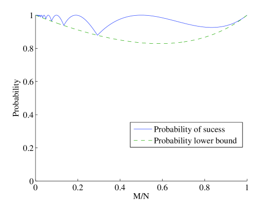
Figure 4: Probability of success of the algorithm using the required number of iterations $q$.

5 Comparison with Grover’s Algorithm

First we will summarise the probabilities of success and the required number of iterations for Grover’s algorithm and the proposed algorithm before giving the comparison. The probability of success of Grover’s algorithm as shown in [4] is as follows:

$$P^{(q_{G})}_{s}=\sin^{2}\left({\left({2q_{G}+1}\right)\theta_{G}}\right)\geq 1-\frac{M}{N},$$ (44)

where $\sin^{2}\left(\theta_{G}\right)={M}/{N},\,\,\,0<\theta_{G}\leq{\pi}/{2}$ and the required number of iterations $q_{G}$ is,

$$q_{G}=\left\lfloor{\frac{\pi}{4\theta_{G}}}\right\rfloor\leq\frac{\pi}{4}\sqrt{\frac{N}{M}}.$$ (45)

For the proposed algorithm, the probability of success is as follows,

$$P_{s}^{(q)}=\left({1-\cos\left(\theta\right)}\right)\left({\frac{\sin^{2}\left({\left({q+1}\right)\theta}\right)}{\sin^{2}\left(\theta\right)}+\frac{\sin^{2}\left({q\theta}\right)}{\sin^{2}\left(\theta\right)}}\right),$$ (46)

where $\cos\left(\theta\right)=1-{M}/{N},\,\,\,0<\theta\leq{\pi}/{2}$ and the required $q$ is,

$$q=\left\lfloor{\frac{\pi}{2\theta}}\right\rfloor\leq\frac{\pi}{2\sqrt{2}}\sqrt{\frac{N}{M}}.$$ (47)

Fig. 5.a shows the probability of success for both algorithms using the required number of iterations. We can see from the plot that the minimum probability that Grover’s algorithm may reach is approximately 50.0% when $M/N\approx 0.5$ while for the proposed algorithm, the minimum probability is 87.88% when $M/N\approx 0.2928$. Grover’s algorithm will behave similar to the single guess technique for $M/N>0.5$ where $q_{G}=0$ in that range so that $P^{(q_{G})}_{s}=M/N$. Although the proposed algorithm is slower than Grover’s algorithm for small $M/N$ by $\sqrt{2}$, Fig. 5.b shows the probability of success for both algorithms for small $M/N$ (hard cases where $M/N<1\times 10^{-3})$, where we can see that the proposed algorithm is more reliable (higher probability) than Grover’s algorithm. For $M/N>1/3$, $q=1$ where the proposed algorithm runs in $O(1)$ to get probability at least 90%, i.e. the problem is easier for multiple matches.

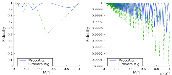
Figure 5: Probability of success using the $q_{G}$ and $q$ for both algorithms: a. $0<{M}/{N}\leq 1$ (left), b. $M/N<1\times 10^{-3}$ (right).

6 Unknown Number of Matches

In case we do not know the number of matches $M$ in advance, we can apply the algorithm shown in [4] for $1\leq M\leq N$ by replacing Grover’s step with the proposed algorithm. The algorithm can be summarised as follows:

• Start with $m=1$ and $\lambda={8}/{7}$. (where $\lambda$ can take any value between 1 and ${4}/{3}$)

• Pick an integer $j$ between 0 and $m-1$ in a uniform random manner.

• Run $j$ iterations of the proposed algorithm on the state:

  $$\frac{1}{{\sqrt{N}}}\sum\limits_{i=0}^{N-1}{\left|i\right\rangle\otimes\left|0\right\rangle}.$$

• Measure the register and assume $i$ is the output.

• If $f(i)=1$, then we found a solution and exit.

• Let $m=min\left(\lambda m,\sqrt{N}\right)$ and go to step 2.

For the sake of simplicity and to be able to compare the performance of this algorithm with that shown in [4], we will try to follow the same style of analysis used in [4]. Before we construct the analysis, we need the following lemmas. The first lemma is straightforward using mathematical induction.

Lemma 6.1.

For any positive integer $m$ and real number $\theta$ such that $0<\theta\leq\pi/2$,

$$\sum\limits_{q=0}^{m-1}{\sin^{2}\left({\left({q+1}\right)\theta}\right)+\sin^{2}\left({q\theta}\right)=m-\frac{{\cos\left(\theta\right)\sin\left({2m\theta}\right)}}{{2\sin\left(\theta\right)}}}.$$

Lemma 6.2.

Assume $M$ is the unknown number of matches such that $1\leq M\leq N$. Let $\theta$ be a real number such that $\cos\left(\theta\right)=1-M/N$ and $0<\theta\leq\pi/2$. Let $m$ be any positive integer. Let $q$ be any integer picked in a uniform random manner between 0 and $m-1$. Measuring the register after applying $q$ iterations of the proposed algorithm starting from the initial state, the probability $P_{m}$ of finding a solution is as follows,

$$P_{m}=\frac{1}{{1+\cos\left(\theta\right)}}\left({1-\frac{{\cos\left(\theta\right)\sin\left({2m\theta}\right)}}{{2m\sin\left(\theta\right)}}}\right),$$

where, $P_{m}>0.2725$ for $m\geq 1/\sin\left(\theta\right)$ and small $M/N$.

Proof.

The average probability of success when applying $q$ iterations of the proposed algorithm when $0\leq q\leq m$ is picked in a uniform random manner is as follows,

$$\begin{array}[]{l}P_{m}=\sum\limits_{q=0}^{m-1}{\frac{1}{m}}P_{s}^{(q)}=\frac{1}{{m\left({1+\cos\left(\theta\right)}\right)}}\sum\limits_{q=0}^{m-1}{\sin^{2}\left({\left({q+1}\right)\theta}\right)+\sin^{2}\left({q\theta}\right)}\\ \,\,\,\,\,\,\,\,=\frac{1}{{1+\cos\left(\theta\right)}}\left({1-\frac{{\cos\left(\theta\right)\sin\left({2m\theta}\right)}}{{2m\sin\left(\theta\right)}}}\right).\\ \end{array}$$

If $m\geq 1/\sin\left(\theta\right)$ and $M\ll N$ then $\cos\left(\theta\right)\approx 1$, so,

$$P_{m}>\frac{1}{2}-\frac{{\sin\left({2m\theta}\right)}}{{4m\sin\left(\theta\right)}}\geq\frac{1}{2}-\frac{{\sin\left({2m\theta}\right)}}{4}>0.2725,$$

where $\sin\left({2m\theta}\right)<0.91$ for $0<\theta\leq\pi/2$.

∎

We calculate the total expected number of iterations as done in Theorem 3 in [4]. Assume that $m_{q}\geq 1/\sin\left(\theta\right)$, and $v_{q}=\left\lceil{\log_{\lambda}m_{q}}\right\rceil$. Notice that, $m_{q}=O\left({\sqrt{N/M}}\right)$ for $1\leq M\leq N$, then:

• The total expected number of iterations to reach the critical stage, i.e. when $m\geq m_{q}$:

  $$\frac{1}{2}\sum\limits_{v=1}^{v_{q}}{\lambda^{v-1}}=\frac{1}{{2\left({\lambda-1}\right)}}m_{q}=3.5m_{q}.$$

• The total expected number of iterations after reaching the critical stage:

  $$\frac{1}{2}\sum\limits_{u=0}^{\infty}{\left({0.7275}\right)^{u}\lambda^{v_{q}+u}=\frac{1}{{2\left({1-0.7275\lambda}\right)}}}m_{q}=2.9m_{q}.$$

The total expected number of iterations whether we reach to the critical stage or not is $6.4m_{q}$ which is in $O(\sqrt{N/M})$ for $1\leq M\leq N$.

When this algorithm employed Grover’s algorithm [4], and based on the condition $m_{G}\geq 1/\sin\left({2\theta_{G}}\right)=O\left({\sqrt{N/M}}\right)$ for $1\leq M\leq{3N}/{4}$, where $m_{G}$ will act as a lower bound for $q_{G}$ in that range. The total expected number of iterations is approximately $8m_{G}$. For $M>{3N}/{4}$, $m_{G}$ will increase exponentially where it will not be able to approximate $q_{G}$. Employing the proposed algorithm instead, and based on the condition $m_{q}\geq 1/\sin\left({\theta}\right)=O\left({\sqrt{N/M}}\right)$ for $1\leq M\leq N$, the total expected number of iterations is approximately $6.4m_{q}$, i.e. the algorithm will be able to handle the whole range, since $m_{q}$ will be able to act as a lower bound for $q$ over $1\leq M\leq N$. Fig. 6 compares between the total expected number of iterations for both algorithms taking $\lambda=8/7$.

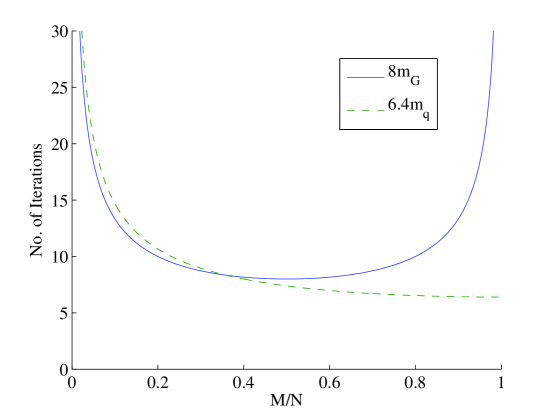
Figure 6: The actual behaviour of the functions representing the total expected number of iterations for Grover’s algorithm $8m_{G}$ and the proposed algorithm $6.4m_{q}$ taking $\lambda=8/7$, where the number of iterations is the flooring of the values (step function).

7 Conclusion

In Grover’s algorithm, the search space is split into two subspaces (the solution and non-solution subspaces) then amplifies the amplitudes of the solution states by iterating the diffusion operator and the oracle [12] to find a match with high probability in $O(\sqrt{N/M})$ for small $M/N$ and in the neighbourhood of $M/N=1/4$ [4]. The main idea of using partial diffusion in quantum search is to split the subspace of the solutions into two smaller subspaces. In each iteration, one of the solution subspaces will be inverted about the mean (together with the non-solution subspace) while the other half will have the sign of their amplitudes changed to the negative sign, preparing it to be inverted about the mean (together again with the non-solution subspace) in the next iteration. The benefit of this alternating inversion is to preserve half the number of the solution states at each iteration so as to resist the de-amplification behaviour of the standard diffusion operator when reaching the so-called turning points and get the solution with high probability in $O(\sqrt{N/M})$ for $1\leq M\leq N$. Apply the oracle $U_{f}$ each iteration will switch the entanglement of the two solution subspaces with the extra qubit workspace to decide which subspace to be inverted about the mean with the non-solution subspace.

An algorithm for unknown number of matches replacing Grover’s step in the algorithm shown in [4] is presented, where we showed that the algorithm will be able to handle the range $1\leq M\leq N$ in $O(\sqrt{N/M})$ compared with $1\leq M\leq 3N/4$ when using Grover’s algorithm.

We showed that the algorithm will be able to handle the whole possible range $1\leq M\leq N$ more reliably using fixed operators in $O\left({\sqrt{N/M}}\right)$ for both known and unknown number of matches which makes it more suitable for practical purposes.

References

• [1] A. Barenco, C. Bennett, R. Cleve, D. P. Divincenzo, N. Margolus, P. Shor, T. Sleator, J. Smolin, and H. Weinfurter. Elementary gates for quantum computation. Physical Review A, 52(5):3457–3467, 1995.
• [2] E. Biham and D. Dan Kenigsberg. Grover’s quantum search algorithm for an arbitrary initial mixed state. Physical Review A, 66:062301, 2002. Also in quant-ph/0306182.
• [3] D. Biron, O. Biham, E. Biham, M. Grassl, and D. A. Lidar. Generalized Grover search algorithm for arbitrary initial amplitude distribution. Los Alamos Physics Preprint Archive, quant-ph/9801066.
• [4] M. Boyer, G. Brassard, P. Høyer, and A. Tapp. Tight bounds on quantum searching. Fortschritte der Physik, 46:493, 1998.
• [5] G. Brassard, P. Høyer, M. Mosca, , and A. Tapp. Quantum amplitude amplification and estimation. Los Alamos Physics Preprint Archive, quant-ph/0005055.
• [6] G. Brassard, P. Høyer, and A. Tapp. Quantum counting. Los Alamos Physics Preprint Archive, quant-ph/9805082.
• [7] G. Chen and S. Fulling. Generalization of Grover’s algorithm to multiobject search in quantum computing, part II: General unitary transformation. Los Alamos Physics Preprint Archive, quant-ph/0007124.
• [8] G. Chen, S. Fulling, and J. Chen. Generalization of Grover’s algorithm to multiobject search in quantum computing, part I: Continuous time and discrete time. Los Alamos Physics Preprint Archive, quant-ph/0007123.
• [9] G. Chen, S. Fulling, and M. Scully. Grover’s algorithm for multiobject search in quantum computing. Los Alamos Physics Preprint Archive, quant-ph/9909040.
• [10] A General Phase Matching Condition for Quantum Searching Algorithm. Li, c. and hwang, c. and hsieh, j. and wang, k. Los Alamos Physics Preprint Archive, quant-ph/0108086.
• [11] A. Galindo and M.A. Martin-Delgado. Family of Grover’s quantum-searching algorithms. Physical Review A, 62:062303, 2000. Also in quant-ph/0009086.
• [12] L. Grover. A fast quantum mechanical algorithm for database search. In Proceedings of the 28th Annual ACM Symposium on the Theory of Computing, pages 212–219, 1996.
• [13] L. Grover. Quantum computers can search rapidly by using almost any transformation. Physical Review Letters, 80(19):4329–4332, 1998.
• [14] P. Høyer. Arbitrary phases in quantum amplitude amplification. Physical Review A, 62:052304, 2000.
• [15] R. Jozsa. Searching in Grover’s algorithm. Los Alamos Physics Preprint Archive, quant-ph/9901021.
• [16] G. L. Long. Grover algorithm with zero theoretical failure rate. Los Alamos Physics Preprint Archive, quant-ph/0106071.
• [17] M. Mosca. Quantum searching, counting and amplitude amplification by eigenvector analysis. In Proceedings of Randomized Algorithms, Workshop of Mathematical Foundations of Computer Science, pages 90–100, 1998.
• [18] M. Nielsen and I. Chuang. Quantum Computation and Quantum Information. Cambridge University Press, Cambridge, United Kingdom, 2000.
• [19] T. J. Rivlin. Chebyshev Polynomials. Wiley, New York, 1990.
• [20] C. Zalka. Grover’s quantum searching algorithm is optimal. Physical Review A, 60(4):2746–2751, 1999.
• [21] A. Younes, J. Rowe and J  Miller. Quantum Search Algorithm with more Reliable Behaviour using Partial Diffusion. Los Alamos Physics Preprint Archive, quant-ph/0312022.