Recursive Calculation of Effective Potential and Variational Resummation

Abstract

We set up a method for a recursive calculation of the effective potential which is applied to a cubic potential with imaginary coupling. The result is resummed using variational perturbation theory (VPT), yielding an exponentially fast convergence.

I Introduction

Perturbation theory is the most commonly used technique for an approximate description of non-exactly solvable systems. However, most perturbation series are divergent and yield acceptable results only after resummation. In recent years, based on a variational approach due to Feynman and Kleinert Feynman2 , a systematic and uniformly convergent variational perturbation theory (VPT) has been developed Kleinertsys ; PathInt3 ; VerenaBuch ; Festschrift . It permits the conversion of divergent weak-coupling into convergent strong-coupling expansions and has been applied successfully in quantum mechanics, quantum statistics, condensed matter physics, and the theory of critical phenomena.

The convergence of VPT has been proved to be exponentially fast PathInt3 ; VerenaBuch , and this has been verified for the ground-state energy of different quantum mechanical model systems. If the underlying potential is mirror-symmetric, one introduces a trial oscillator whose frequency $\Omega$ is regarded as a variational parameter and whose influence is minimized according to the principle of minimal sensitivity Stevenson . In this way, the ground-state energy of the quartic anharmonic oscillator was analyzed up to very high orders in Refs. JankeC1 ; JankeC2 .

If the potential is not mirror-symmetric, the center of fluctuations no longer lies at the origin but at some nonzero place $X$. In VPT, this situation is accounted for by regarding the nonvanishing center of fluctuations $X$ as a second variational parameter. An extreme example is a complete antisymmetric potential, such as $V(x)=Ax^{3}$, which for real $A$ does not correspond to a stable system. Interestingly, if the parameter $A$ is chosen to be imaginary, so that there does not exist a classical system at all, the quantum-mechanical system turns out to be well-defined, and the spectrum of the Hamilton operator

$$H=-\frac{1}{2}\frac{\partial^{2}}{\partial x^{2}}+ix^{3}$$ (1)

is real and positive. This remarkable property of the non-Hermitian Hamilton operator, found in Refs. BenderPT ; BenderPT2 ; BenderPT3 ; BenderPT4 ; BenderPT5 , can be attributed to the fact that it possesses a different symmetry: it is invariant under the combined application of the parity and the time-reversal operation.

In this paper, we apply VPT to the ${\cal PT}$-symmetric Hamilton operator (1). In a first naive approach, we ignore the necessary shift $X$ of the center of fluctuations and resum the weak-coupling series of the ground-state energy for the anharmonic oscillator

$$V(x)=\frac{\omega^{2}}{2}x^{2}+igx^{3}$$ (2)

in the strong-coupling limit. In this limit, the potential (2) reduces to the purely cubic potential of (1). It turns out that the VPT results approach the corresponding numerical value for the ground-state energy of (1) with increasing order, but the rate of convergence is not satisfactory. Afterwards, we allow for a nonvanishing center of fluctuations $X$ by using the effective potential, whose calculation is accomplished by an efficient recursion scheme. This refined approach improves the convergence of the results drastically.

In Section II, we derive the weak-coupling series for the ground-state energy of (2) by evaluating connected vacuum diagrams. In Section III, we show how this perturbation series can be obtained more efficiently by means of the Bender-Wu recursion method Bender/Wu . In Section IV, we resum the weak-coupling series for the ground-state energy of (2) by applying VPT and examine the resulting convergence. In Section V, we determine the effective potential with the background method DeWitt ; Jackiw from one-particle irreducible vacuum diagrams. In Section VI, we set up new recursion relations for a more efficient calculation of the effective potential. In Section VII, we finally treat the resulting expansion with VPT and examine the improved convergence.

II Perturbation Theory

The perturbation series for the ground-state energy of the anharmonic oscillator (2) can be calculated from connected vacuum diagrams. Up to the fourth order in the coupling constant $g$, the ground-state energy is given by the Feynman diagrams

$$E = \frac{\hbar\omega}{2}-\lim_{T\to 0}k_{B}T\bigg{\{}\hskip 2.84526pt\frac{1}{8}\hskip 5.69054pt\parbox{42.67912pt}{\centerline{\hbox{ \immediate\ignorespaces\immediate\ignorespaces\immediate\ignorespaces\immediate\ignorespaces\immediate\ignorespaces\leavevmode\includegraphics{graph.1}\ignorespaces\immediate\ignorespaces\immediate\ignorespaces\immediate\ignorespaces\immediate\ignorespaces\immediate\ignorespaces\immediate\ignorespaces\immediate\ignorespaces\immediate\ignorespaces\immediate\ignorespaces\immediate\ignorespaces\immediate\ignorespaces\immediate\ignorespaces\immediate\ignorespaces\immediate\ignorespaces\immediate\ignorespaces\immediate\ignorespaces\immediate\ignorespaces \immediate\ignorespaces }} }+\frac{1}{12}\hskip 5.69054pt\parbox{19.91692pt}{\centerline{\hbox{ \immediate\ignorespaces\immediate\ignorespaces\immediate\ignorespaces\immediate\ignorespaces\immediate\ignorespaces\leavevmode\includegraphics{graph.2}\ignorespaces\immediate\ignorespaces\immediate\ignorespaces\immediate\ignorespaces\immediate\ignorespaces\immediate\ignorespaces\immediate\ignorespaces\immediate\ignorespaces\immediate\ignorespaces\immediate\ignorespaces\immediate\ignorespaces\immediate\ignorespaces\immediate\ignorespaces\immediate\ignorespaces\immediate\ignorespaces \immediate\ignorespaces }} }$$

$$+\hskip 2.84526pt\frac{1}{24}\hskip 5.69054pt\parbox{25.60747pt}{\centerline{\hbox{ \immediate\ignorespaces\immediate\ignorespaces\immediate\ignorespaces\immediate\ignorespaces\immediate\ignorespaces\leavevmode\includegraphics{graph.3}\ignorespaces\immediate\ignorespaces\immediate\ignorespaces\immediate\ignorespaces\immediate\ignorespaces\immediate\ignorespaces\immediate\ignorespaces\immediate\ignorespaces\immediate\ignorespaces\immediate\ignorespaces\immediate\ignorespaces\immediate\ignorespaces\immediate\ignorespaces\immediate\ignorespaces\immediate\ignorespaces\immediate\ignorespaces\immediate\ignorespaces\immediate\ignorespaces \immediate\ignorespaces }} }+\frac{1}{16}\hskip 5.69054pt\parbox{25.60747pt}{\centerline{\hbox{ \immediate\ignorespaces\immediate\ignorespaces\immediate\ignorespaces\immediate\ignorespaces\immediate\ignorespaces\leavevmode\includegraphics{graph.4}\ignorespaces\immediate\ignorespaces\immediate\ignorespaces\immediate\ignorespaces\immediate\ignorespaces\immediate\ignorespaces\immediate\ignorespaces\immediate\ignorespaces\immediate\ignorespaces\immediate\ignorespaces\immediate\ignorespaces\immediate\ignorespaces\immediate\ignorespaces\immediate\ignorespaces\immediate\ignorespaces\immediate\ignorespaces\immediate\ignorespaces\immediate\ignorespaces \immediate\ignorespaces }} }+\frac{1}{8}\hskip 5.69054pt\parbox{42.67912pt}{\centerline{\hbox{ \immediate\ignorespaces\immediate\ignorespaces\immediate\ignorespaces\immediate\ignorespaces\immediate\ignorespaces\leavevmode\includegraphics{graph.5}\ignorespaces\immediate\ignorespaces\immediate\ignorespaces\immediate\ignorespaces\immediate\ignorespaces\immediate\ignorespaces\immediate\ignorespaces\immediate\ignorespaces\immediate\ignorespaces\immediate\ignorespaces\immediate\ignorespaces\immediate\ignorespaces\immediate\ignorespaces\immediate\ignorespaces\immediate\ignorespaces\immediate\ignorespaces\immediate\ignorespaces\immediate\ignorespaces\immediate\ignorespaces\immediate\ignorespaces\immediate\ignorespaces \immediate\ignorespaces }} }$$

$$+\hskip 2.84526pt\frac{1}{16}\hskip 5.69054pt\parbox{65.44133pt}{\centerline{\hbox{ \immediate\ignorespaces\immediate\ignorespaces\immediate\ignorespaces\immediate\ignorespaces\immediate\ignorespaces\leavevmode\includegraphics{graph.6}\ignorespaces\immediate\ignorespaces\immediate\ignorespaces\immediate\ignorespaces\immediate\ignorespaces\immediate\ignorespaces\immediate\ignorespaces\immediate\ignorespaces\immediate\ignorespaces\immediate\ignorespaces\immediate\ignorespaces\immediate\ignorespaces\immediate\ignorespaces\immediate\ignorespaces\immediate\ignorespaces\immediate\ignorespaces\immediate\ignorespaces\immediate\ignorespaces\immediate\ignorespaces\immediate\ignorespaces\immediate\ignorespaces\immediate\ignorespaces \immediate\ignorespaces }} }+\frac{1}{48}\hskip 5.69054pt\parbox{48.36967pt}{\centerline{\hbox{ \immediate\ignorespaces\immediate\ignorespaces\immediate\ignorespaces\immediate\ignorespaces\immediate\ignorespaces\leavevmode\includegraphics{graph.7}\ignorespaces\immediate\ignorespaces\immediate\ignorespaces\immediate\ignorespaces\immediate\ignorespaces\immediate\ignorespaces\immediate\ignorespaces\immediate\ignorespaces\immediate\ignorespaces\immediate\ignorespaces\immediate\ignorespaces\immediate\ignorespaces\immediate\ignorespaces\immediate\ignorespaces\immediate\ignorespaces\immediate\ignorespaces\immediate\ignorespaces\immediate\ignorespaces\immediate\ignorespaces\immediate\ignorespaces\immediate\ignorespaces\immediate\ignorespaces\immediate\ignorespaces\immediate\ignorespaces \immediate\ignorespaces }} }+{\cal O}(g^{6})\bigg{\}}\hskip 2.84526pt,$$

with the propagator

$$\parbox{19.91692pt}{\centerline{\hbox{ \begin{picture}(6.0,6.0)\immediate\ignorespaces\immediate\ignorespaces\immediate\ignorespaces\immediate\ignorespaces\immediate\ignorespaces\put(0.0,0.0){\includegraphics{graph.8}}\ignorespaces\immediate\ignorespaces\immediate\ignorespaces\immediate\ignorespaces\immediate\ignorespaces\immediate\ignorespaces\immediate\ignorespaces\immediate\ignorespaces\immediate\ignorespaces\immediate\ignorespaces\immediate\ignorespaces\immediate\ignorespaces\immediate\ignorespaces\immediate\ignorespaces\immediate\ignorespaces\immediate\ignorespaces \immediate\ignorespaces{\put(-1.0,3.0){\makebox(0.0,0.0)[r]{${\scriptstyle i}$}}\put(7.0,3.0){\makebox(0.0,0.0)[l]{${\scriptstyle j}$}}}\end{picture} }} }\hskip 14.22636pt\to\hskip 5.69054ptG_{\omega}(\tau_{i},\tau_{j})=\frac{\hbar}{2\omega}e^{-\omega|\tau_{i}-\tau_{j}|}$$ (4)

and the vertices

$$\parbox{19.91692pt}{\centerline{\hbox{ \begin{picture}(6.0,6.0)\immediate\ignorespaces\immediate\ignorespaces\immediate\ignorespaces\immediate\ignorespaces\immediate\ignorespaces\put(0.0,0.0){\includegraphics{graph.9}}\ignorespaces\immediate\ignorespaces\immediate\ignorespaces\immediate\ignorespaces\immediate\ignorespaces\immediate\ignorespaces\immediate\ignorespaces\immediate\ignorespaces\immediate\ignorespaces\immediate\ignorespaces\immediate\ignorespaces\immediate\ignorespaces\immediate\ignorespaces\immediate\ignorespaces\immediate\ignorespaces\immediate\ignorespaces\immediate\ignorespaces\immediate\ignorespaces\immediate\ignorespaces \immediate\ignorespaces{\put(3.0,2.0){\makebox(0.0,0.0)[t]{${\scriptstyle i}$}}}\end{picture} }} }\hskip 14.22636pt\to\hskip 5.69054pt-\frac{6ig}{\hbar}\int_{0}^{\hbar\beta}d\tau_{i}\hskip 2.84526pt.$$ (5)

Evaluating the Feynman diagrams (II) leads to the following analytical expression for the ground-state energy:

$$E=\hbar\omega\left[\frac{1}{2}+\frac{11g^{2}\hbar}{8\omega^{5}}-\frac{465g^{4}\hbar^{2}}{32\omega^{10}}+{\cal O}(g^{6})\right]\hskip 2.84526pt.$$ (6)

Since evaluating Feynman diagrams of higher orders is cumbersome, only low perturbation orders are feasible by this procedure. If we want to study higher orders, we better use the Bender-Wu recursion relations Bender/Wu .

III Bender-Wu Recursion Relations

The Schrödinger eigenvalue equation for the anharmonic oscillator (2),

$$-\frac{\hbar^{2}}{2}\psi^{\prime\prime}(x)+\left(\frac{\omega^{2}}{2}x^{2}+igx^{3}\right)\psi(x)=E\psi(x)\hskip 2.84526pt,$$ (7)

is solved as follows: We write the wave function $\psi(x)$ as

$$\psi(x)=\left(\frac{\omega}{\pi\hbar}\right)^{1/4}\exp\left[-\frac{\hat{x}^{2}}{2}+\phi(\hat{x})\right]\hskip 2.84526pt,$$ (8)

with the abbreviation $\hat{x}=x\sqrt{\omega/\hbar}$, and expand the exponent in powers of the dimensionless coupling constant $\hat{g}=g\sqrt{\hbar/\omega^{5}}$ by using

$$\phi(\hat{x})=\sum_{k=1}^{\infty}\hat{g}^{k}\phi_{k}(\hat{x})\hskip 2.84526pt.$$ (9)

The $\phi_{k}(\hat{x})$ are expanded in powers of the rescaled coordinate $\hat{x}$:

$$\phi_{k}(\hat{x})=\sum_{m=1}^{k+2}c_{m}^{(k)}\hat{x}^{m}\hskip 2.84526pt.$$ (10)

For the ground-state energy we make the ansatz

$$E=\hbar\omega\left(\frac{1}{2}+\sum_{k=1}^{\infty}\hat{g}^{k}\epsilon_{k}\right)\hskip 2.84526pt.$$ (11)

Inserting (8) – (11) into (7), we obtain to first order

$$c_{1}^{(1)}=-i,\quad c_{2}^{(1)}=0,\quad c_{3}^{(1)}=-\frac{i}{3},\quad\epsilon_{1}=0\hskip 2.84526pt.$$ (12)

For $k\geq 2$, we find the following recursion relation for the expansion coefficients in (10):

$$c_{m}^{(k)} = \frac{(m+2)(m+1)}{2m}\hskip 2.84526ptc_{m+2}^{(k)}$$

$$+\hskip 2.84526pt\frac{1}{2m}\sum_{l=1}^{k-1}\sum_{n=1}^{m+1}n(m+2-n)\hskip 2.84526ptc_{n}^{(l)}\hskip 2.84526ptc_{m+2-n}^{(k-l)}\hskip 2.84526pt,$$

with $c_{m}^{(k)}\equiv 0$ for $m>k+2$. The expansion coefficients of the ground-state energy follow from

$$\epsilon_{k}=-c_{2}^{(k)}-\frac{1}{2}\sum_{l=1}^{k-1}c_{1}^{(l)}\hskip 2.84526ptc_{1}^{(k-l)}\hskip 2.84526pt.$$ (14)

Table 1 shows the coefficients $\epsilon_{k}$ up to the 10th order. We observe that all odd orders vanish for symmetry reasons and that the first two even orders agree, indeed, with the earlier result (6).

$k$	$1$	$2$	$3$	$4$	$5$
$\epsilon_{k}$	$0$	${\displaystyle\frac{11}{8}}$	$0$	${\displaystyle-\frac{465}{32}}$	$0$
$k$	$6$	$7$	$8$	$9$	$10$
$\epsilon_{k}$	${\displaystyle\frac{39709}{128}}$	$0$	${\displaystyle-\frac{19250805}{2048}}$	$0$	${\displaystyle\frac{2944491879}{8192}}\hskip 5.69054pt$

Table 1: Expansion coefficients for the ground-state energy of the anharmonic oscillator (2) up to the 10th order.

IV Resummation of Ground-State Energy

In this section, we consider the strong-coupling limit of the perturbation series (11). Rescaling the coordinate according to $x\to xg^{-1/5}$, the Schrödinger equation (7) becomes

$$-\frac{\hbar^{2}}{2}\hskip 2.84526pt\frac{\partial^{2}}{\partial x^{2}}\hskip 2.84526pt\psi(x)+\left(\frac{1}{2}g^{-4/5}\omega^{2}x^{2}+ix^{3}\right)\psi(x) =$$

$$g^{-2/5}E\hskip 2.84526pt\psi(x)\hskip 2.84526pt.$$

Expanding the wave function and the energy in powers of the coupling constant yields

$$\psi(x)=\psi_{0}(\hat{x})+\hat{g}^{-4/5}\psi_{1}(\hat{x})+\hat{g}^{-8/5}\psi_{2}(\hat{x})+\ldots$$ (16)

and

$$E = \hbar\omega\hskip 2.84526pt\hat{g}^{2/5}\left(b_{0}+\hat{g}^{-4/5}b_{1}+\hat{g}^{-8/5}b_{2}+\ldots\right)\hskip 2.84526pt.$$ (17)

By considering (IV) in the limit $g\to\infty$, we find that the leading strong-coupling coefficient $b_{0}$ equals the ground-state energy associated with the Hamilton operator (1). A precise numerical value for this ground-state energy was given by C.M. Bender BenderPT ; BenderPrivat :

$$b_{0}=0.762851773\ldots\hskip 2.84526pt.$$ (18)

The weak-coupling series (11) is of the form

$$E^{(N)}(\alpha,\omega)=\hbar\omega\left[\frac{1}{2}+\sum_{k=1}^{N}\left(\frac{\hbar\alpha}{\omega^{5}}\right)^{k}\epsilon_{2k}\right]\hskip 2.84526pt,$$ (19)

with the abbreviation $\alpha=g^{2}$. Table 1 suggests that (19) represents a divergent Borel series which is resummable by applying VPT Kleinertsys ; PathInt3 ; VerenaBuch ; Festschrift . To this end, an artificial parameter is introduced in the perturbation series, which is most easily obtained by Kleinert’s square-root trick

$$\omega\to\Omega\sqrt{1+\alpha r}\hskip 2.84526pt,$$ (20)

with

$$r=\frac{\omega^{2}-\Omega^{2}}{\alpha\Omega^{2}}\hskip 2.84526pt.$$ (21)

Thus, one replaces the frequency $\omega$ in the weak-coupling series (19) according to (20) and re-expands the resulting expression in powers of $\alpha$ up to the order $\alpha^{N}$. Afterwards, the auxiliary parameter $r$ is replaced according to (21). The ground-state energy thus becomes dependent on the variational parameter $\Omega$: $E^{(N)}(\alpha,\hskip 2.84526pt\omega)\to E^{(N)}(\alpha,\hskip 2.84526pt\omega,\hskip 2.84526pt\Omega)$. The influence of $\Omega$ is then optimized according to the principle of minimal sensitivity Stevenson , i.e. one approximates the ground-state energy to $N$th order by

$$E^{(N)}=E^{(N)}(\alpha,\hskip 2.84526pt\omega,\hskip 2.84526pt\Omega^{(N)})\hskip 2.84526pt,$$ (22)

where $\Omega^{(N)}$ denotes that value of the variational parameter for which $E^{(N)}(\alpha,\hskip 2.84526pt\omega,\hskip 2.84526pt\Omega)$ has an extremum or a turning point.

Consider, as an example, the weak-coupling series (19) to first order:

$$E^{(1)}(\alpha,\hskip 2.84526pt\omega)=\frac{\hbar\omega}{2}+\alpha\frac{11\hbar^{2}}{8\omega^{4}}\hskip 2.84526pt.$$ (23)

Inserting (20), re-expanding in $\alpha$ to first order, and taking into account (21), we obtain

$$E^{(1)}(\alpha,\hskip 2.84526pt\omega,\hskip 2.84526pt\Omega)=\frac{\hbar\Omega}{4}+\frac{\hbar\omega^{2}}{4\Omega}+\alpha\frac{11\hbar^{2}}{8\Omega^{4}}\hskip 2.84526pt.$$ (24)

Extremizing this and going to large coupling constants, we obtain the strong-coupling behavior of the variational parameter:

$$\Omega^{(1)}=\omega\hat{\alpha}^{1/5}\left(\Omega^{(1)}_{0}+\Omega^{(1)}_{1}\hat{\alpha}^{-2/5}+\Omega^{(1)}_{2}\hat{\alpha}^{-4/5}+\ldots\right),$$ (25)

with the abbreviation $\hat{\alpha}=\hat{g}^{2}$ and the coefficients

$$\Omega_{0}^{(1)}=\sqrt[5]{22},\hskip 2.84526pt\Omega_{1}^{(1)}=\frac{1}{5\sqrt[5]{22}},\hskip 2.84526pt\Omega_{2}^{(1)}=\frac{1}{25\sqrt[5]{10648}},\hskip 2.84526pt\ldots\hskip 2.84526pt.$$ (26)

Inserting the result (25), (26) into (24), we obtain the strong-coupling series (17) with the first-order coefficients

$$b_{0}^{(1)}=\frac{5\sqrt[5]{22}}{16},\hskip 2.84526pt\hskip 2.84526ptb_{1}^{(1)}=\frac{4}{\sqrt[5]{22}},\hskip 2.84526pt\hskip 2.84526ptb_{2}^{(1)}=\frac{-1}{100\sqrt[5]{22}}\hskip 2.84526pt,\hskip 2.84526pt\ldots\hskip 2.84526pt.$$ (27)

The numerical value of the leading strong-coupling coefficient is $b_{0}^{(1)}\approx 0.5799$. Thus, to first order, the relative deviation of the result from the precise value (18) is

$$\frac{|b^{(1)}_{0}-b_{0}|}{b_{0}}\approx 24\%\hskip 2.84526pt.$$ (28)

Despite this relatively poor agreement, it turns out that the VPT results for $b_{0}^{(N)}$ in higher orders converge towards the exact value (18). In Refs. PathInt3 ; VerenaBuch it is proved that VPT in general yields approximations whose relative deviation from the exact value vanishes exponentially. In our case we have

$$\frac{|b_{0}^{(N)}-b_{0}|}{b_{0}}\propto\exp\left(-CN^{3/5}\right)\hskip 2.84526pt,$$ (29)

where the exponent $3/5$ is determined by the structure of the strong-coupling series (17).

In Fig. 1 the exponential convergence of our variational results is shown up to the $20$th order. Fitting the logarithm of the relative deviation to a straight line yields

$$\ln\frac{|b_{0}^{(N)}-b_{0}|}{b_{0}}=-0.96(11)N^{3/5}-1.83(44)\hskip 2.84526pt.$$ (30)

In the following, we show how this exponential convergence is improved drastically by allowing for a shift of the center of fluctuations.

V Diagrammatic Approach to Effective Potential

In the presence of a constant external current $j$, the quantum statistical partition function reads

$$Z(j):=\oint{\cal D}x\hskip 2.84526pt\exp\left\{-\frac{1}{\hbar}\hskip 2.84526pt{\cal A}[x](j)\right\}\hskip 1.42262pt,$$ (31)

where ${\cal A}[x](j)$ is the Euclidean action:

$${\cal A}[x](j)=\int_{0}^{\hbar\beta}d\tau\left[\frac{1}{2}\dot{x}^{2}(\tau)+V(x(\tau))-jx(\tau)\right]\hskip 2.84526pt.$$ (32)

The free energy thus becomes a function of the external current:

$$F(j)=-\frac{1}{\beta}\ln Z(j)\hskip 2.84526pt.$$ (33)

The path average,

$$X=\frac{1}{Z(j)}\oint{\cal D}x\left[\int_{0}^{\hbar\beta}\frac{d\tau}{\hbar\beta}\hskip 2.84526ptx(\tau)\hskip 2.84526pt\right]\exp\left\{-\frac{1}{\hbar}\hskip 2.84526pt{\cal A}[x](j)\right\}\hskip 2.84526pt,$$

then follows from the first derivative of the free energy with respect to the external current:

$$X=-\frac{\partial F(j)}{\partial j}\hskip 2.84526pt.$$ (35)

Assuming that the last identity can be inverted to yield the current $j$ as a function of the average $X$, one defines the effective potential $V_{\rm eff}(X)$ as the Legendre transform of the free energy with respect to the external current:

$$V_{\rm eff}(X)=F(j(X))+j(X)X\hskip 2.84526pt.$$ (36)

Furthermore, the first derivative of the effective potential gives back the external current $j$:

$$\frac{\partial V_{\rm eff}(X)}{\partial X}=j(X)\hskip 2.84526pt.$$ (37)

Thus, the free energy $F\equiv F(j=0)$ can be obtained by extremizing the effective potential,

$$F=V_{\rm eff}(X_{\rm e})\hskip 2.84526pt,$$ (38)

with

$$\left.\frac{\partial V_{\rm eff}(X)}{\partial X}\right|_{X=X_{\rm e}}=0\hskip 2.84526pt.$$ (39)

In the zero-temperature limit, extremizing the effective potential then yields the ground-state energy.

The effective potential is usually not calculated by performing explicitly the Legendre transformation (36) but by a diagrammatic technique derived via the so-called background method Jackiw ; DeWitt . There, the effective potential is expanded in powers of the Planck constant $\hbar$, and the expansion terms are one-particle irreducible vacuum diagrams. The result is

$$V_{\rm eff}(X)=V(X)+\frac{\hbar}{2}\mbox{Tr}\ln G^{-1}+V^{(\rm int)}(X)\hskip 2.84526pt,$$ (40)

where the trace-log term is given by the ground-state energy of a harmonic oscillator of $X$-dependent frequency $\tilde{\omega}=\sqrt{V^{\prime\prime}(X)}$:

$$\frac{\hbar}{2}\mbox{Tr}\ln G^{-1}=\frac{\hbar\tilde{\omega}}{2}\hskip 2.84526pt.$$ (41)

The interaction term $V^{(\rm int)}(X)$ contains the sum of all one-particle irreducible vacuum diagrams. For the anharmonic oscillator (2), the relevant subset of the diagrams in (II) is

$$V^{(\rm int)}(X) = -\lim_{T\to 0}k_{B}T\bigg{\{}\hskip 2.84526pt\frac{1}{12}\hskip 5.69054pt\parbox{19.91692pt}{\centerline{\hbox{ \immediate\ignorespaces\immediate\ignorespaces\immediate\ignorespaces\immediate\ignorespaces\immediate\ignorespaces\leavevmode\includegraphics{graph.10}\ignorespaces\immediate\ignorespaces\immediate\ignorespaces\immediate\ignorespaces\immediate\ignorespaces\immediate\ignorespaces\immediate\ignorespaces\immediate\ignorespaces\immediate\ignorespaces\immediate\ignorespaces\immediate\ignorespaces\immediate\ignorespaces\immediate\ignorespaces\immediate\ignorespaces\immediate\ignorespaces \immediate\ignorespaces }} }+\frac{1}{24}\hskip 5.69054pt\parbox{25.60747pt}{\centerline{\hbox{ \immediate\ignorespaces\immediate\ignorespaces\immediate\ignorespaces\immediate\ignorespaces\immediate\ignorespaces\leavevmode\includegraphics{graph.11}\ignorespaces\immediate\ignorespaces\immediate\ignorespaces\immediate\ignorespaces\immediate\ignorespaces\immediate\ignorespaces\immediate\ignorespaces\immediate\ignorespaces\immediate\ignorespaces\immediate\ignorespaces\immediate\ignorespaces\immediate\ignorespaces\immediate\ignorespaces\immediate\ignorespaces\immediate\ignorespaces\immediate\ignorespaces\immediate\ignorespaces\immediate\ignorespaces \immediate\ignorespaces }} }$$ (42)

$$+\hskip 2.84526pt\frac{1}{16}\hskip 5.69054pt\parbox{25.60747pt}{\centerline{\hbox{ \immediate\ignorespaces\immediate\ignorespaces\immediate\ignorespaces\immediate\ignorespaces\immediate\ignorespaces\leavevmode\includegraphics{graph.12}\ignorespaces\immediate\ignorespaces\immediate\ignorespaces\immediate\ignorespaces\immediate\ignorespaces\immediate\ignorespaces\immediate\ignorespaces\immediate\ignorespaces\immediate\ignorespaces\immediate\ignorespaces\immediate\ignorespaces\immediate\ignorespaces\immediate\ignorespaces\immediate\ignorespaces\immediate\ignorespaces\immediate\ignorespaces\immediate\ignorespaces\immediate\ignorespaces \immediate\ignorespaces }} }\bigg{\}}+\hskip 2.84526pt{\cal O}(\hbar^{4})\hskip 2.84526pt.$$

These one-particle irreducible vacuum diagrams are derived most easily by an efficient graphical recursion method Phi3Phi4 . The frequency of the propagators is now given by:

$$\tilde{\omega}=\sqrt{\omega^{2}+6igX}\hskip 2.84526pt.$$ (43)

By evaluating the diagrams (42) we obtain

$$V_{\rm eff}(X) = \frac{\omega^{2}}{2}X^{2}+igX^{3}+\frac{\hbar}{2}\sqrt{\omega^{2}+6igX}$$

$$+\frac{\hbar^{2}g^{2}}{4(\omega^{2}+6igX)^{2}}-\frac{51\hbar^{3}g^{4}}{32\left(\omega^{2}+6igX\right)^{9/2}}+{\cal O}(\hbar^{4})\hskip 2.84526pt.$$

The ground-state energy of the anharmonic oscillator (2) is found by extremizing the effective potential (V). To this end, we expand the extremal background according to

$$X_{\rm e}=i(X_{0}+\hbar X_{1}+\hbar^{2}X_{2}+\hbar^{3}X_{3})+{\cal O}(\hbar^{4})\hskip 2.84526pt.$$ (45)

Inserting (45) into the vanishing first derivative of (V) and re-expanding in $\hbar$, we obtain a system of equations which are solved by

$$X_{0}=0\hskip 2.84526pt,\quad\quad X_{1}=-\frac{3g}{2\omega^{3}}\hskip 2.84526pt,\quad\quad X_{2}=\frac{33g^{3}}{2\omega^{8}}\hskip 2.84526pt.$$ (46)

Inserting (45), (46) into (V) and re-expanding in $\hbar$ yields again the ground-state energy (6).

In order to go to higher orders, we shall now develop a recursion relation for the effective potential.

VI Recursive Approach to Effective Potential

In the presence of a constant external current $j$, the Schrödinger eigenvalue equation for the anharmonic oscillator (2) reads

$$-\frac{\hbar^{2}}{2}\psi^{\prime\prime}(x)+\left(\frac{\omega^{2}}{2}x^{2}+igx^{3}-jx\right)\psi(x)=E\psi(x)\hskip 2.84526pt.$$ (47)

Taking into account the Legendre identities (36), (37), Eq. (47) becomes

$$-\frac{\hbar^{2}}{2}\psi^{\prime\prime}(x)+\left(\frac{\omega^{2}}{2}x^{2}+igx^{3}-V_{\rm eff}^{\prime}(X)x\right)\psi(x)$$

$$=\Big{[}V_{\rm eff}(X)-V_{\rm eff}^{\prime}(X)X\Big{]}\psi(x)\hskip 2.84526pt.$$ (48)

If the coupling constant $g$ vanishes, Eq. (48) is solved by

$$\psi(x) = {\cal N}\hskip 2.84526pt\exp\left(\hat{X}\hat{x}-\frac{\hat{x}^{2}}{2}\right)\hskip 2.84526pt,$$ (49)

$$V_{\rm eff}(X) = \hbar\omega\left(\frac{1}{2}+\frac{\hat{X}}{2}\right)\hskip 2.84526pt,$$ (50)

where the path average has been rescaled by the oscillator length: $\hat{X}=X\sqrt{\omega/\hbar}$. For a nonvanishing coupling constant $g$, we solve the differential equation (48) by the expansions

$$\psi(x) = {\cal N}\hskip 2.84526pt\exp\left[\hat{X}\hat{x}-\frac{\hat{x}^{2}}{2}+\phi(\hat{x})\right],$$ (51)

$$V_{\rm eff}(X) = \hbar\omega\left[\frac{1}{2}+\frac{\hat{X}^{2}}{2}+\sum_{k=1}^{\infty}\hat{g}^{k}V_{k}(\hat{X})\right]\hskip 2.84526pt.$$ (52)

For the correction to the wave function, $\phi(\hat{x})$, we make again the ansatz (9), (10). Thus, we obtain from (48) for $k=1$:

$$c_{1}^{(1)}=\frac{i}{2}+2i\hat{X}^{2},\quad\hskip 2.84526pt\hskip 2.84526ptc_{2}^{(1)}=-\frac{i\hat{X}}{2},\quad\hskip 2.84526pt\hskip 2.84526ptc_{3}^{(1)}=-\frac{i}{3}\hskip 2.84526pt,$$ (53)

$$\hskip 39.83385ptV_{1}(\hat{X})=\frac{3i\hat{X}}{2}+i\hat{X}^{3}\hskip 2.84526pt.$$ (54)

For $k\geq 2$ one finds for $m\geq 2$ the following recursion relation for the expansion coefficients of the wave function

$$c_{m}^{(k)} = \frac{(m+2)(m+1)}{2m}\hskip 2.84526ptc_{m+2}^{(k)}+\frac{\hat{X}(m+1)}{m}\hskip 2.84526ptc_{m+1}^{(k)}$$ (55)

$$+\hskip 2.84526pt\frac{1}{2m}\sum_{l=1}^{k-1}\sum_{n=1}^{m+1}n(m+2-n)\hskip 2.84526ptc_{n}^{(l)}\hskip 2.84526ptc_{m+2-n}^{(k-l)}\hskip 2.84526pt,$$

with $c_{m}^{(k)}\equiv 0$ for $m>k+2$. For $m=1$, we have

$$c_{1}^{(k)} = 3c_{3}^{(k)}+2\hat{X}c_{2}^{(k)}+V_{k}^{\prime}(\hat{X})$$ (56)

$$+\sum_{l=1}^{k-1}\left(c_{2}^{(k-l)}c_{1}^{(l)}+c_{1}^{(k-l)}c_{2}^{(l)}\right)\hskip 2.84526pt.$$

The expansion coefficients of the effective potential follow from

$$V_{k}(\hat{X}) = -c_{2}^{(k)}-3\hat{X}c_{3}^{(k)}-2\hat{X}^{2}c_{2}^{(k)}$$

$$-\hat{X}\sum_{l=1}^{k-1}\left(c_{2}^{(k-l)}c_{1}^{(l)}+c_{1}^{(k-l)}c_{2}^{(l)}\right)-\frac{1}{2}\sum_{l=1}^{k-1}c_{1}^{(l)}\hskip 2.84526ptc_{1}^{(k-l)}.$$

$l$	$0$	$1$	$2$
$V^{(l)}(X)$	${\displaystyle\frac{\omega^{2}}{2}X^{2}+igX^{3}}$	${\displaystyle\frac{\tilde{\omega}}{2}}$	${\displaystyle\frac{g^{2}}{4\tilde{\omega}^{4}}}$
$l$	$3$	$4$	$5$
$V^{(l)}(X)$	${\displaystyle-\frac{51g^{4}}{32\tilde{\omega}^{9}}}$	${\displaystyle\frac{3331g^{6}}{128\tilde{\omega}^{14}}}$	${\displaystyle-\frac{1371477g^{8}}{2048\tilde{\omega}^{19}}}$

Table 2: Expansion coefficients for the effective potential of (2) up to five loops.

Using these results, the effective potential can be determined recursively, yielding an expansion in the coupling constant $g$:

$$V_{\rm eff}(X) = \frac{\hbar\omega}{2}+\frac{\omega^{2}}{2}X^{2}+ig\left(\frac{3\hbar X}{2\omega}+X^{3}\right)$$

$$+\hskip 2.84526ptg^{2}\frac{\hbar(\hbar+9\omega X^{2})}{4\omega^{4}}-ig^{3}\frac{3\hbar X(4\hbar+9\omega X^{2})}{4\omega^{6}}$$

$$-\hskip 2.84526ptg^{4}\frac{3\hbar(17\hbar^{2}+288\hbar X^{2}+270X^{4}\omega^{2})}{32\omega^{9}}+{\cal O}(g^{5})\hskip 2.84526pt.$$

This result is in agreement with the expansion of (V) in powers of $g$ and can be carried to higher orders without effort. The expansion coefficients for the $\hbar$-expansion

$$V_{\rm eff}(X)=\sum_{l=0}^{N}\hbar^{l}V^{(l)}(X)+{\cal O}(\hbar^{N+1})$$ (59)

can then be obtained easily Diplomarbeit . Iterating the recursion relations (55) – (VI) up to the order $g^{8}$, we obtain the effective potential up to five loops as shown in Tab. 2.

VII Resummation of Effective Potential

We now apply VPT to the loop expansion of the effective potential (59). Since the Planck constant $\hbar$ is now the expansion parameter rather than the coupling constant $g$, Kleinert’s square-root trick will be modified accordingly:

$$\omega\to\Omega\sqrt{1+\hbar r}\hskip 2.84526pt,$$ (60)

with

$$r=\frac{\omega^{2}-\Omega^{2}}{\hbar\Omega^{2}}\hskip 2.84526pt.$$ (61)

As an example, we consider again the first order:

$$V_{\rm eff}^{(1)}(X)=\frac{\omega^{2}}{2}X^{2}+igX^{3}+\frac{\hbar}{2}\sqrt{\omega^{2}+6igX}\hskip 2.84526pt.$$ (62)

After substituting $\omega$ according to (60), re-expanding in $\hbar$, and taking into account (61), we obtain

$$V_{\rm eff}^{(1)}(X,\Omega)=\frac{\omega^{2}}{2}X^{2}+igX^{3}+\frac{\hbar}{2}\sqrt{\Omega^{2}+6igX}\hskip 2.84526pt.$$ (63)

In order to calculate an approximation for the ground-state energy, we now optimize in $\Omega$ and extremize in $X$, yielding

$$\frac{\partial}{\partial\Omega}V_{\rm eff}^{(1)}(X,\Omega)\bigg{|}_{X=X^{(1)},\hskip 2.84526pt\Omega=\Omega^{(1)}} = 0\hskip 2.84526pt,$$ (64)

$$\frac{\partial}{\partial X}V_{\rm eff}^{(1)}(X,\Omega)\bigg{|}_{X=X^{(1)},\hskip 2.84526pt\Omega=\Omega^{(1)}} = 0\hskip 2.84526pt.$$ (65)

1-loop VPT	0.742751023
2-loop VPT	0.764570478
3-loop VPT	0.758783545
4-loop VPT	0.762843684
5-loop VPT	0.762849959
Numerical	0.762851773

Table 3: Variational results for the ground-state energy of (1) compared to the numerical result (18) of Refs. BenderPT ; BenderPrivat .

Equation (64) is solved by

$$\Omega^{(1)}=0\hskip 2.84526pt.$$ (66)

Afterwards, we obtain from (65):

$$X^{(1)}+\frac{\omega^{2}}{3ig}+\frac{\hbar}{2\sqrt{6ig}(X^{(1)})^{3/2}}=0\hskip 2.84526pt.$$ (67)

This equation allows us to determine the strong-coupling behavior of $X$:

$$X^{(1)} = -i\hat{g}^{-1/5}\sqrt{\frac{\hbar}{\omega}}$$

$$\times\hskip 2.84526pt\left(X_{0}^{(1)}+X_{1}^{(1)}\hat{g}^{-4/5}+X_{2}^{(1)}\hat{g}^{-8/5}+\ldots\right)\hskip 2.84526pt,$$

where the coefficients read

$$X_{0}^{(1)}=\frac{1}{\sqrt[5]{24}},\hskip 2.84526ptX_{1}^{(1)}=-\frac{2}{15},\hskip 2.84526ptX_{2}^{(1)}=\frac{\sqrt[5]{24}}{75},\hskip 2.84526pt\ldots\hskip 2.84526pt.$$ (69)

Inserting the results (66), (VII), (69) into (63) yields the strong-coupling behavior of the ground-state energy (17), with the new coefficients:

$$b_{0}^{(1)}=\frac{5}{2\sqrt[5]{432}},\hskip 2.84526ptb_{1}^{(1)}=-\frac{1}{4\sqrt[5]{18}},\hskip 2.84526ptb_{2}^{(1)}=\frac{1}{15\sqrt[5]{24}},\hskip 2.84526pt\ldots\hskip 2.84526pt.$$ (70)

The new numerical value of the leading strong-coupling coefficient is $b_{0}^{(1)}\approx 0.7428$, which is in much better agreement with (18) than the previous value of (27):

$$\frac{|b^{(1)}_{0}-b_{0}|}{b_{0}}\approx 3\%\hskip 2.84526pt.$$ (71)

Thus, the variational path average has led to a significant improvement of the first-order result. Table 3 summarizes our results for $b_{0}^{(N)}$ up to the fifth order.

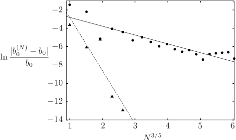
Figure 1: Convergence of the results for the strong-coupling coefficient $b_{0}$ obtained from resummation of the weak-coupling series of the ground-state energy (circles). The resummation involving a variational path average $X$ converges much faster (triangles). The lines represent fits of the respective data to straight lines.

Figure 1 shows the much faster exponential convergence up to the fifth order. A best fit of the data yields

$$\ln\frac{|b_{0}^{(N)}-b_{0}|}{b_{0}}=-5.8(1.6)N^{3/5}+3.0(3.0)\hskip 2.84526pt$$ (72)

which is to be compared with (30).

VIII Conclusion and Outlook

We have developed a recursive technique to determine the effective potential, which is far more efficient than diagrammatic methods. In combination with VPT, this leads to a fast converging determination of the ground-state energy of quantum-mechanical systems with non-mirror symmetric potentials. It will be interesting to analyze in a similar way systems with a coordinate dependent mass term, where only a lowest order effective potential has been calculated so far KleinertEffMass . Interesting future applications will address the effective potential of $\phi^{4}$ theories in $4-\epsilon$ dimensions to obtain equations of state near to a critical point. A first attempt in this direction is Ref. Brazil .

References

• (1) R.P. Feynman and H. Kleinert: Phys. Rev. A 34, 5080 (1986).
• (2) H. Kleinert: Phys. Lett. A 173, 332 (1993).
• (3) H. Kleinert: Path Integrals in Quantum Mechanics, Statistics, Polymer Physics, and Financial Markets, Third Edition (World Scientific, Singapore, 2004).
• (4) H. Kleinert and V. Schulte-Frohlinde: Critical Properties of $\phi^{4}$-Theories (World Scientific, Singapore, 2001).
• (5) W. Janke, A. Pelster, H.-J. Schmidt, and M. Bachmann (Editors): Fluctuating Paths and Fields – Dedicated to Hagen Kleinert on the Occasion of his 60th Birthday (World Scientific, Singapore, 2001).
• (6) P.M. Stevenson: Phys. Rev. D 23, 2916 (1981).
• (7) W. Janke and H. Kleinert: Phys. Rev. Lett. 75, 2787 (1995).
• (8) H. Kleinert and W. Janke: Phys. Lett. A 206, 283 (1995).
• (9) C.M. Bender and S. Boettcher: Phys. Rev. Lett. 80, 5243 (1998).
• (10) C.M. Bender, S. Boettcher, and P.N. Meisinger: J. Math. Phys. 40, 2201 (1999).
• (11) C.M. Bender, S. Boettcher, and P.N. Meisinger: Ref. Festschrift , p. 105.
• (12) C.M. Bender, D.C. Brody, and H.F. Jones: Phys. Rev. Lett. 89, 270401 (2002).
• (13) C.M. Bender, D.C. Brody, and H.F. Jones: Am. J. Phys. 71, 1095 (2003).
• (14) C.M. Bender and T.T. Wu: Phys. Rev. 184, 1231 (1969); Phys. Rev. D 7, 1620 (1973).
• (15) B. De Witt: Dynamical Theory of Groups and Fields (Gordon and Breach, New York, 1965).
• (16) R. Jackiw: Phys. Rev. D 9, 1686 (1974).
• (17) A. Pelster and H. Kleinert: Physica A 323, 370 (2003).
• (18) C.M. Bender (private communication).
• (19) More details can be found in: S.F. Brandt: Beyond Effective Potential via Variational Perturbation Theory (Diplom thesis, Freie Universität Berlin, 2004):
http://www.physik.fu-berlin.de/~sbrandt.
• (20) H. Kleinert and A. Chervyakov: Phys. Lett. A 299, 319 (2002).
• (21) C.M.L. de Aragão and C.E.I. Carneiro: Phys. Rev. D 68, 065010 (2003).