Fast Quantum Algorithm for Numerical Gradient Estimation

Abstract

Given a blackbox for $f$, a smooth real scalar function of $d$ real variables, one wants to estimate $\nabla f$ at a given point $\mathbf{x}=\left(x_{1},x_{2},\ldots,x_{d}\right)$ with $n$ bits of precision. On a classical computer this requires a minimum of $d+1$ blackbox queries, whereas on a quantum computer it requires only one query regardless of $d$. The number of bits of precision to which $f$ must be evaluated matches the classical requirement in the limit of large $n$.

In the context of many numerical calculations, blackbox query complexity is a natural measure of algorithmic efficiency. For example, in optimization problems, the function evaluations are frequently the most time consuming part of the computation, and an efficient optimization algorithm is therefore one which uses as few function evaluations as possible Press et al. (1992).

Here we investigate the query complexity of numerically estimating the gradient of a blackbox function at a given point. We find that gradients can be estimated on a quantum computer using a single blackbox query. The algorithm which achieves this can be viewed as a generalization of the Bernstein-Vazirani Bernstein and Vazirani (1993) algorithm, which has been described in other contexts Mosca (1999); Høyer (1999); Cleve et al. (1998); Bennett et al. (1997). The blackbox in this algorithm has always previously been described as evaluating a function over the integers rather than approximating a continuous function with finite precision. Gradient finding is the first known practical variant of this algorithm. In Mosca (1999), the question as to whether the algorithm could be adapted for any task of practical interest was presented as an open problem, which this paper resolves.

The blackbox that we consider takes as its input $d$ binary strings, each of length $n$, along with $n_{o}$ ancilla qubits which should be set to zero. The blackbox writes its output into the ancilla bits using addition modulo $2^{n_{o}}$ and preserves the input bits. This is a standard technique for making any function reversible, which it must be for a quantum computer to implement it.

The purpose of the blackbox is to evaluate some function $f:\mathbb{R}^{d}\to\mathbb{R}$ with $n_{o}$ bits of precision on a finite domain. It does so in fixed-point notation. That is, the inputs and outputs to the function $f$, which are real numbers within a finite range, are approximated by the inputs and outputs to the blackbox, which are integers ranging from 0 to $2^{n}$, and 0 to $2^{n_{o}}$, respectively, via appropriate scaling and offset.

For numerical gradient estimation to work, in the classical or quantum case, $f$ and its first partial derivatives must be continuous in the vicinity of the point $(x_{1},x_{2},\ldots,x_{d})$ at which the gradient is to be evaluated. Classically, to estimate $\nabla f$ at $\mathbf{x}$ in $d$ dimensions, one can evaluate $f$ at $\mathbf{x}$ and at $d$ additional points, each displaced from $f$ along one of the $d$ dimensions.

In practice, it may be desirable in the classical gradient estimation algorithm to perform the function evaluations displaced by $\pm l/2$ from $\mathbf{x}$ along each dimension so that the region being sampled is centered at $\mathbf{x}$. In this case $2d$ function evaluations are required instead of $d+1$. $\partial f/\partial x_{1}$ will then be given by $(f(x_{1}+l/2,\ldots)-f(x_{1}-l/2,\ldots))/l$, and similarly for the other partial derivatives. Inserting the Taylor expansion for $f$ about $\mathbf{x}$ into this expression shows that the quadratic terms will cancel, leaving an error of order $l^{2}$ and higher. One must choose $l$ sufficiently small that these terms are negligible.

Now we consider the quantum case. It suffices to show how to perform a quantum gradient estimation at $\mathbf{x}=\mathbf{0}$, since the gradient at other points can be obtained by trivially redefining $f$. To estimate the gradient at the origin, start with $d$ input registers of $n$ qubits each, plus a single output register of $n_{o}$ qubits, all initialized to zero. Perform the Hadamard transform on the input registers, write the value 1 into the output register and then perform an inverse Fourier transform on it. This yields the superposition

$$\frac{1}{\sqrt{N^{d}N_{o}}}\sum_{\delta_{1}=0}^{N-1}\sum_{\delta_{2}=0}^{N-1}\ldots\sum_{\delta_{d}=0}^{N-1}|\delta_{1}\rangle\ldots|\delta_{d}\rangle\sum_{a=0}^{N_{o}-1}e^{i2\pi a/N_{o}}|a\rangle$$

where $N\equiv 2^{n}$ and $N_{o}\equiv 2^{n_{o}}$. In vector notation,

$$=\frac{1}{\sqrt{N^{d}N_{o}}}\sum_{\bm{\delta}}|\bm{\delta}\rangle\sum_{a}e^{i2\pi a/N_{o}}|a\rangle$$

Next, use the blackbox to compute $f$ and add it modulo $N_{o}$ into the output register. The output register is an eigenstate of addition modulo $N_{o}$. The eigenvalue corresponding to addition of x is $e^{i2\pi x/N_{o}}$. Thus by writing into the output register via modular addition, we obtain a phase proportional to $f$. This technique is sometimes called phase kickback. The resulting state is

$$\frac{1}{\sqrt{N^{d}N_{o}}}\sum_{\bm{\delta}}e^{i2\pi\frac{N}{ml}f(\frac{l}{N}(\bm{\delta}-\frac{\mathbf{N}}{2}))}|\bm{\delta}\rangle\sum_{a}e^{i2\pi a/N_{o}}|a\rangle$$

where $\mathbf{N}$ is the $d$-dimensional vector $(N,N,N,\ldots)$, and $l$ is the size of the region over which $f$ is approximately linear. $l$ and $\mathbf{N}$ are used to convert from the components of $\bm{\delta}$, which are nonnegative integers represented by bit strings, to rationals evenly spaced over a small region centered at the origin. Similarly, the blackbox output is related to the value of $f$ by $a\to a\oplus\lceil\frac{NN_{o}}{ml}f\rfloor\mod N_{o}$. $m$ is the size of the interval which bounds the components of $\nabla f$. This ensures proper scaling of the final result into a fixed point representation, that is, as an integer from 0 to $2^{n}$.

For sufficiently small $l$,

$$\approx\frac{1}{\sqrt{N^{d}N_{o}}}\sum_{\bm{\delta}}e^{i\frac{2\pi N}{ml}\left(f(\mathbf{0})+\frac{l}{N}(\bm{\delta}-\frac{\mathbf{N}}{2})\cdot\nabla f\right)}|\bm{\delta}\rangle\sum_{a}e^{i2\pi a/N_{o}}|a\rangle.$$

Writing out the vector components, and ignoring global phase, the input registers are now approximately in the state

$$\begin{split}=\frac{1}{\sqrt{N^{d}}}\sum_{\delta_{1}\ldots\delta_{d}}e^{i\frac{2\pi}{m}\left(\delta_{1}\frac{\partial f}{\partial x_{1}}+\delta_{2}\frac{\partial f}{\partial x_{2}}+\ldots+\delta_{d}\frac{\partial f}{\partial x_{d}}\right)}\times\\ |\delta_{1}\rangle|\delta_{2}\rangle\ldots|\delta_{d}\rangle.\end{split}$$

This is a product state:

$$=\frac{1}{\sqrt{N^{d}}}\left(\sum_{\delta_{1}}e^{i\frac{2\pi}{m}\delta_{1}\frac{\partial f}{\partial x_{1}}}|\delta_{1}\rangle\right)\ldots\left(\sum_{\delta_{d}}e^{i\frac{2\pi}{m}\delta_{d}\frac{\partial f}{\partial x_{d}}}|\delta_{d}\rangle\right).$$

Fourier transform each of the registers, obtaining

$$\left|\frac{N}{m}\frac{\partial f}{\partial x_{1}}\right>\left|\frac{N}{m}\frac{\partial f}{\partial x_{2}}\right>\ldots\left|\frac{N}{m}\frac{\partial f}{\partial x_{d}}\right>.$$

Then simply measure in the computational basis to obtain the components of $\nabla f$ with $n$ bits of precision. Because $f$ will in general not be perfectly linear, even over a small region, there also will be nonzero amplitude to measure other values close to the exact gradient, as will be discussed later.

Normally, the quantum Fourier transform is thought of as mapping the discrete planewave states to the computational basis states:

$$\frac{1}{\sqrt{N}}\sum_{j=0}^{N}e^{2\pi ijk/N}|j\rangle\to|k\rangle$$

where $0<k<N$. However, negative $k$ is also easily dealt with, since

$$\frac{1}{\sqrt{N}}\sum_{j=0}^{N}e^{-2\pi ij|k|/N}\to|N-|k|\rangle.$$

Thus negative components of $\nabla f$ pose no difficulties for the quantum gradient estimation algorithm provided that bounds for the values of the components are known, which is a requirement for any algorithm using fixed-point arithmetic.

In general the number of bits of precision necessary to represent a set of values is equal to $\log_{2}(r/\delta)$, where $r$ is the range of values, and $\delta$ is the smallest difference in values one wishes to distinguish. Thus for classical gradient estimation with $n$ bits of precision, one needs to evaluate $f$ to

$$\log_{2}\left[\frac{\mathrm{max}(f)-\mathrm{min}(f)}{\frac{ml}{2^{n}}}\right]$$ (1)

bits of precision.

An important property of the quantum Fourier transform is that it can correctly distinguish between exponentially many discrete planewave states with high probability without requiring the phases to be exponentially precise Nielsen and Chuang (2000). It is not hard to show that if each phase is accurate to within $\theta$ then the inner product between the ideal state and the actual state is at least $\cos\theta$, and therefore the algorithm will still succeed with probability at least $\cos^{2}\theta$.

As shown earlier, the phase acquired by “kickback” is equal to $\frac{2\pi N}{ml}f$, and therefore, for the phase to be accurate to within $\pm\theta$, $f$ must be evaluated to within $\pm\frac{ml}{2\pi N}\theta$. Thus, recalling that $N=2^{n}$,

$$n_{o}=\log_{2}\left[\frac{\max f-\min f}{\frac{ml}{2^{n}}\frac{\theta}{2\pi}}\right].$$ (2)

As an example, if $\theta=\pi/8$, then the algorithm will behave exactly as in the idealized case with approximately $85\%$ probability, and $N_{o}$ will exceed the classically required precision by four bits, for a given value $l$. $l$ also differs between the quantum and classical cases, as will be discussed later. Thus $n_{o}$ differs from the classically required precision only by an additive constant which depends on $\theta$ and $l$. Because the classical and quantum precision requirements are both proportional to $n$, this difference becomes negligible in the limit of large $n$.

The only approximation made in the description of the quantum gradient estimation algorithm was expanding $f$ to first order. Therefore the lowest order error term will be due to the quadratic part of $f$. The behavior of the algorithm in the presence of such a quadratic term provides an idea of its robustness. Furthermore, in order to minimize the number of bits of precision to which $f$ must be evaluated, $l$ should be chosen as large as possible subject to the constraint that $f$ be locally linear. The analysis of the quadratic term provides a more precise description of this constraint.

The series of quantum Fourier transforms on different registers can be thought of as a single $d$-dimensional quantum Fourier transform. Including the quadratic term, the state which this Fourier transform is acting on has amplitudes

$$f(\bm{\delta})=\frac{1}{N^{d/2}}\mathrm{exp}\left[i2\pi\left(\bm{\delta}\cdot\nabla f+\frac{l}{2mN}\bm{\delta}^{T}H\bm{\delta}\right)\right],$$

where $H$ is the Hessian matrix of $f$. After the Fourier transform, the amplitudes should peak around the correct value of $\nabla f$. Here we are interested in the width of the peak, which should not be affected by $\nabla f$, so for simplicity it will be set to 0. The Fourier transform will yield amplitudes of

$$\tilde{f}(\mathbf{k})=\frac{1}{N^{d}}\sum_{\bm{\delta}}\mathrm{exp}\left[i2\pi\left(\frac{l}{2mN}\bm{\delta}^{T}H\bm{\delta}-\frac{1}{N}\mathbf{k}\cdot\bm{\delta}\right)\right].$$

Ignoring global phase and doing a change of variables ($\mathbf{u}=\delta/N$),

$$\approx\int_{-1/2}^{1/2}\ldots\int_{-1/2}^{1/2}\mathrm{exp}\left[i2\pi\left(\frac{Nl}{2m}\mathbf{u}^{T}H\mathbf{u}-\mathbf{k}\cdot\mathbf{u}\right)\right]\mathrm{d}^{d}\mathbf{u}$$

This integral can be approximated using the method of stationary phase. $\nabla\phi=\frac{Nl}{2m}\left(H^{T}+H\right)\mathbf{u}-\mathbf{k}$ but Hessians are symmetric, so $\nabla\phi=\frac{Nl}{m}H\mathbf{u}-\mathbf{k}.$ Thus (again ignoring global phase),

$$\tilde{f}(\mathbf{k})\approx\left\{\begin{array}[]{ll}\sqrt{\frac{1}{\mathrm{Det}\left(\frac{Nl}{m}H\right)}}&\textrm{if}\ \exists\ \mathbf{u}\in C\ \textrm{s.t.}\ \frac{Nl}{m}H\mathbf{u}-\mathbf{k}=0\\ &\\ 0&\textrm{otherwise}\end{array}\right.$$

where $C$ is the region $-1/2<u_{i}<1/2\quad\forall\ i$. So according to the stationary phase approximation, the peak is simply a region of uniform amplitude, with zero amplitude elsewhere. Geometrically, this region is what is obtained by applying the linear transformation $\frac{Nl}{m}H$ to the $d$-dimensional unit hypercube.

Since we have set $\nabla f=0$, the variance of $\frac{N}{m}\frac{\partial f}{\partial x_{i}}$ will be

$$\sigma_{i}^{2}=\frac{1}{\mathrm{Det}A}\int_{D}k_{i}^{2}d^{d}\mathbf{k}\quad\textrm{where}\quad A=\frac{Nl}{m}H$$

and $D$ is the region of nonzero amplitude. Doing a change of variables with $A$ as the Jacobian,

$$\sigma_{i}^{2}=\frac{1}{\mathrm{Det}A}\int_{C}(A\mathbf{k}^{\prime})_{i}^{2}\mathrm{Det}A\ d^{d}\mathbf{k}^{\prime}$$

where $C$ is again the unit hypercube centered at the origin. In components,

$$\sigma_{i}^{2}=\int_{C}\left(\sum_{j}A_{ij}k_{j}^{\prime}\right)^{2}d^{d}\mathbf{k}^{\prime}.$$

The expectation values on a hypercube of uniform probability are $\left<x_{i}x_{j}\right>=\frac{1}{12}\delta_{ij}$, thus

$$\sigma_{i}^{2}=\frac{1}{12}\sum_{j}A_{ij}^{2}=\frac{N^{2}l^{2}}{12m^{2}}\sum_{j}\left(\frac{\partial^{2}f}{\partial x_{i}\partial x_{j}}\right)^{2}.$$

This quadratic dependence on $N$ is just as expected since, at the end of the computation, the register that we are measuring is intended to contain $\frac{N}{m}\frac{\partial f}{\partial x}$. Therefore the uncertainty in $\partial f/\partial x_{i}$ is approximately

$$\frac{l}{2\sqrt{3}}\sqrt{\sum_{j}\left(\frac{\partial^{2}f}{\partial x_{i}\partial x_{j}}\right)^{2}}$$ (3)

independent of $N$. In the classical algorithm which uses $2d$ function evaluations, the cubic term introduces an error of $\sigma\sim\frac{l^{2}}{24}D_{3}$ where $D_{3}$ is the typical magnitude of third partial derivatives of $f$. If the $2^{\textrm{nd}}$ partial derivatives of $f$ have a magnitude of approximately $D_{2}$ then the typical uncertainty in the quantum case will be $\sigma\sim\frac{lD_{2}\sqrt{d}}{2\sqrt{3}}$. To obtain a given uncertainty $\sigma$,

$$l\sim\left\{\begin{array}[]{ll}2\sqrt{\frac{6\sigma}{D_{3}}}&\textrm{classical}\\ &\\ \frac{2\sqrt{3}\sigma}{D_{2}\sqrt{d}}&\textrm{quantum}\end{array}\right.$$

Recalling Eq. (1) and (2), the number of bits of precision to which $f$ must be evaluated depends logarithmically on $l$. However, in the limit of large $n$, the number of bits will match the classical requirement.

The level of accuracy of the stationary phase approximation can be assessed by comparison to numerical solutions of example cases. In one dimension, Eq. (3) reduces to $\sigma^{2}=\frac{\alpha^{2}N^{2}}{3}$ where $\alpha=\frac{l}{2m}\frac{\partial^{2}f}{\partial x^{2}}$. Figures 2 and 1 display the close agreement between numerical results and the analytical solution obtained using stationary phase.

Figure 1: Comparison between error estimates obtained in the stationary phase approximation (solid line) and numerical results (points) for the one dimensional case. Here the $2^{\textrm{nd}}$ derivative remains constant ($\alpha=0.02$), and the number of bits to which the gradient is being evaluated is varied.

Figure 2: Analytical error estimates (solid line) are again tested against numerical results (the points) in the one dimensional case, varying the $2^{\textrm{nd}}$ derivative instead of the number of bits. Here $N=80$.

A two dimensional example provides a nontrivial test of the stationary phase method’s prediction of the peak shape. If the Hessian is such that

$$\frac{N}{m}H=0.1\left[\begin{array}[]{rr}1&1\\ 1&-1\end{array}\right]$$

then, according to the stationary phase approximation, the peak should be a square of side length $\frac{\sqrt{2}}{10}l$ with a $45^{\circ}$ rotation. This is in reasonable agreement with the numerical result, as shown in figure 3.

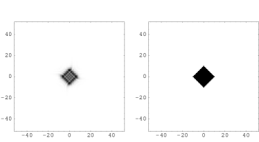
Figure 3: On the left, the probability, as numerically calculated, is shown. The areas of highest probability appear darkest. On the right, the region of nonzero probability, as calculated in the stationary phase approximation, is shaded in black.

Because this algorithm requires only one blackbox query, one might expect that it could be run recursively to efficiently obtain higher derivatives. In this case, another instance of the same algorithm serves as the blackbox. However, the algorithm itself differs from the blackbox in that the blackbox has scalar output which it adds modulo $N_{o}$ to the existing value in the output register, and it does not incur any input-dependent global phase. An additive scalar output can be obtained by minor modification to this algorithm, but the most straightforward techniques for eliminating the global phase require an additional blackbox query, thus necessitating $2^{n}$ queries for the evaluation of an $n^{th}$ partial derivative, just as in the classical case.

The problem of global phase when recursing quantum algorithms as well as the difficulties inherent in recursing approximate or probabilistic algorithms are not specific to gradient finding but are instead fairly general.

Efficient gradient estimation may be useful, for example, in some optimization and rootfinding algorithms. Furthermore, upon discretization, the problem of minimizing a functional is converted into the problem of minimizing a function of many variables, which might benefit from gradient descent techniques. A speedup in the minimization of functionals may in turn enable more efficient solution of partial differential equations via the Euler-Lagrange equation. The analysis of the advantage which this technique can provide in quantum numerical algorithms remains open for further research.

The author thanks P. Shor, E. Farhi, L. Grover, J. Traub, and M. Rudner for useful discussions, and MIT’s Presidential Graduate Fellowship program for financial support.

References

- Press et al. (1992) W. H. Press, S. A. Teukolsky, W. T. Vetterling, and B. P. Flannery, Numerical Recipes in C (Cambridge University Press, 1992), 2nd ed.
- Bernstein and Vazirani (1993) E. Bernstein and U. Vazirani, Proceedings of the 25 ACM Symposium on the Theory of Computing pp. 11–20 (1993).
- Mosca (1999) M. Mosca, Ph.D. thesis, University of Oxford (1999).
- Høyer (1999) P. Høyer, Physical Review A 59, 3280 (1999).
- Cleve et al. (1998) R. Cleve, A. Ekert, C. Macchiavello, and M. Mosca, Proceedings of the Royal Society of London, Series A 454, 339 (1998).
- Bennett et al. (1997) C. H. Bennett, G. Brassard, P. Høyer, and U. Vazirani, SIAM Journal of Computing 26, 1510 (1997).
- Nielsen and Chuang (2000) M. A. Nielsen and I. L. Chuang, Quantum Computation and Quantum Information (Cambridge University Press, 2000), (See exercise 5.6).