Qubit Decoherence and Non-Markovian Dynamics
at Low Temperatures via an Effective Spin-Boson Model

Abstract

Quantum Brownian oscillator model (QBM), in the Fock-space representation, can be viewed as a multi-level spin-boson model. At sufficiently low temperature, the oscillator degrees of freedom are dynamically reduced to the lowest two levels and the system behaves effectively as a two-level (E2L) spin-boson model (SBM) in this limit. We discuss the physical mechanism of level reduction and analyze the behavior of E2L-SBM from the QBM solutions. The availability of close solutions for the QBM enables us to study the non-Markovian features of decoherence and leakage in a SBM in the non-perturbative regime (e.g. without invoking the Born approximation) in better details than before. Our result captures very well the characteristic non-Markovian short time low temperature behavior common in many models.

1 Introduction

Recent development in quantum information processing and quantum computation has attracted much attention to the study of discrete quantum systems with finite degrees of freedom. The most commonly used model is an array of interacting two-level systems (2LS) each of which representing a qubit. As the system almost always interacts with its environment, quantum decoherence in the system usually is the most serious obstacle of actual implementation of quantum information processors [1, 2, 3]. For this reason a detailed understanding of quantum decoherence in open systems is crucial. There are a handful models useful for such studies, the quantum Brownian motion(QBM) [4, 5, 6, 7] is one, the spin-boson model [4, 8] is another: the system in the former case is a harmonic oscillator and in the latter case a 2LS, both interacting with an environment of a harmonic oscillator bath (HOB).

Most qubit models presently employed are the results of picking out the levels most relevant to the description of the qubit from a multi-level structure. In atom optics, internal electronic excitations are often approximated by a 2LS consisting of the ground state and the excited state. A similar model is used for the study of low temperature tunneling process where the two levels degrees of freedom represent the quasi ground states in a double well potential. The simplification to two-levels allows for detailed analytical or numerical treatment, but this remains an approximation applicable only when the effect of higher levels are negligible, e.g. , at low enough temperature when higher levels are not populated. However, in the presence of gate operation, the existence of higher levels causes a leakage of the 2LS due to transitions to other levels. Some extra perturbation may be necessary to select or restrict multi-level structure into the particular levels of interest[9]. In order to make a quantitative estimation of decoherence with a leakage effect, it is more desirable to study open system models which maintain the multi-level structure.

In the present paper, we study the aspects of realistic qubits naturally arising from QBM, taking advantage of a fairly good understanding from the detailed studies over the last few decades. In particular, we focus on harmonic QBM, which can be viewed as an $\infty$-level spin-boson model. Commonly used two-level spin-boson model can be obtained by restricting the harmonic oscillator Fock space to the lowest two levels. This correspondence allows for a detailed analysis of the spin-boson model from the known results of QBM. In particular, we will focus on the non-Markovian aspects of decoherence. Non-Markovian dynamics, often neglected in the literature (models are mainly based on a Markov approximation) for technical simplicity, is actually of crucial importance for the realistic implementations of quantum information processing. The ‘effective’ model we consider here invokes a two level simplification from a multi-level structure. How realistic this is certainly depends on the way the qubits are defined and realized in the multi-level structure usually encountered in actual experimental conditions. Nevertheless our model is able to capture the characteristic short time behavior common in many physical examples.

Beyond the commonly assumed Ohmic spectrum for the bath, generic non-Ohmic environments can be studied with this model. Contrary to the Ohmic case, the sub-Ohmic environment (including $1/f^{\alpha}$ type) causes nontrivial long time behavior such as anomalous diffusion or localization [8] owing to the long range temporal bath correlation. As demonstrated in [10], the influence of slow environment can be dynamically decoupled from the system by using relatively slow pulses[11]. In the present paper, we will mainly focus on the opposite case of supra-Ohmic environments[4, 8, 25]. Owing to the ultra-short time bath correlations, nontrivial short-time system dynamics enters, which is particularly difficult to describe by means of other models or approximations. The decoherece time scale in the supra-Ohmic environment can be much shorter than the one in the Ohmic case and thus is hard to remove by external pulses. Thus supra-Ohmic environment can be a major obstacle for the realization of quantum computation and information processing.

We need to emphasize that to fully follow the coherence of an open system where self-consistency is required, because of the back-action from the environment, we need to study non-Markovian processs. We will also argue that, for a generic class of environment, Markovian approximations are not strictly valid. To facilitate comparison with results in related papers we will compare our methods with other commonly used approximations to the spin-boson model, such as the Born approximation and the Born-Markov rotating-wave approximation[12] for two-level and multi-level systems.

The outline of this paper is as follows: In Sec. 2 we specify the model and cast it in the influence functional formalism in the presence of an external field. In Section 3 we outline our idea of an effective 2LS using the QBM approach. Then we make correspondence between the phase space representation discussed in Sec. 2 with the Fock space representation. We compare our approach with other methods based on Born-Markov and rotating-wave-approximation. Our results are presented in Sec. 4.1. In Sec. 4.2 we discuss the limitations and potential extensions of this approach.

2 QBM in the presence of an external field

2.1 The model

Our model consists of a Brownian particle interacting with a thermal bath in the presence of an external field. We follow the notion developed in [6, 13]. (We use the units in which $k_{B}=\hbar=1$.) The Hamiltonian for this model can be written as

$$H=H_{S}+H_{B}+H_{I}+H_{F},$$ (1)

where the dynamics of the system $S$ (with coordinate $x$ and momentum $p$) is described by the Hamiltonian

$$H_{S}=\frac{{p}^{2}}{2M}+V_{0}(x),$$ (2)

and the (bare) potential $V_{0}(x)$ is related to the physical potential by a counter term $\Delta{V}$ i.e. $V_{0}(x)=V({x})+\Delta{V}$ (see below). The Hamiltonian of the bath is assumed to be composed of harmonic oscillators with natural frequencies $\omega_{n}$ and masses $m_{n}$,

$$H_{B}=\sum_{n=1}^{N}(\frac{{p}_{n}^{2}}{2m_{n}}+\frac{m_{n}\omega_{n}^{2}{q}_{n}^{2}}{2}).$$ (3)

where (${q}_{1},...,{q}_{N},{p}_{1},...,{p}_{N})$ are the coordinates and their conjugate momenta. The interaction between the system S and the bath B is assumed to be bilinear,

$$H_{I}={x}\sum_{n=1}^{N}c_{n}{q}_{n},$$ (4)

where $c_{n}$ is the coupling constant between the Brownian oscillator and the $n$th bath oscillator with coordinate $q_{n}$. The coupling constants are related to the spectral density $J_{B}(\omega)$ of the bath by,

$$J_{B}(\omega)\equiv\pi\sum_{n}\frac{c_{n}^{2}}{2m_{n}\omega_{n}}\delta(\omega-\omega_{n}).$$ (5)

We asssume the spectral density has the form

$$J_{B}(\omega)=2M\gamma\omega^{\nu}e^{-\omega/\Lambda},$$ (6)

where $\nu=1$ is Ohmic, $\nu<1$ is sub-Ohmic , and $\nu>1$ is supra-Ohmic. We will discuss the Ohmic and supra-Ohmic ($\nu=3$) cases in detail.

The counter term $\Delta V$ depends on $c_{n}$, $m_{n}$, $\omega_{n}$, $p$ and $x$ and is given by

$$\Delta V=\left\{\begin{array}[]{ccc}2M\gamma\Lambda x^{2}/\pi&&(\nu=1)\\ 2M\gamma\Lambda p^{2}/M^{2}\pi+2M\gamma\Lambda^{3}x^{2}/\pi&&(\nu=3).\end{array}\right.$$ (9)

This term is introduced to cancel the shift in the mass and frequency of the Brownian oscillator due to its interaction with the bath which will become divergent when the frequency cutoff $\Lambda\rightarrow\infty$. As is customary, we consider the renormalized quantities after including a counter term as the physical observables with specified values.

For a linear QBM, the potential is

$$V(x)=\frac{M\Omega^{2}x^{2}}{2},$$ (10)

where $\Omega$ is the natural frequency of the system oscillator

Finally, the Hamiltonian for the external field is

$$H_{F}=-xE(t),$$ (11)

where $E(t)$ is the external field.

2.2 The Influence Functional

In this subsection, we make connection with the treatment of QBM based on the influence functional[14] with a phase space representation for the Wigner function[15]. First we consider the case without an environment. We define the transition element between the initial state $|x_{0}~{}q_{0}\rangle$ at $t=0$ and the final state $|x~{}q\rangle$ at time $t$ to be

$${K}(x,q;t\mid x_{0},q_{0};0)\equiv\langle x~{}q|e^{-iHt}|x_{0}~{}q_{0}\rangle.$$ (12)

The Liouville equation for the density matrix is

$$i\frac{\partial}{\partial t}{\rho}(t)=\left[H,{\rho}(t)\right],$$ (13)

where $\left[,\right]$ is the commutator. In the coordinate representation, the density matrix becomes

$${\rho}(x,x^{\prime},q,q^{\prime},t)\equiv\langle x~{}q|{\rho}(t)|x^{\prime}~{}q^{\prime}\rangle$$ (14)

with the collective notation for bath variables $q\equiv\{q_{n}\}$. The time evolution of the density matrix is given by

$${\rho}(x,x^{\prime},q,q^{\prime},t)=\int dx_{0}dx^{\prime}_{0}dq_{0}dq^{\prime}_{0}{K}(x,q;t\mid x_{0},q_{0};0){\rho}(x_{0},x^{\prime}_{0},q_{0},q^{\prime}_{0},0){K}^{*}(x^{\prime},q^{\prime};t\mid x^{\prime}_{0},q^{\prime}_{0};0),$$ (15)

In the present paper, we assume that the characteristic time scale for the bath is much shorter than the system. Under this condition, we may integrate out the bath harmonic oscillator variables to obtain an equation for the reduced density matrix ${\rho}_{r}(x,x^{\prime})\equiv\int dq{\rho}(x,x^{\prime},q,q,t)$. For a factorized initial condition between the system and the bath, which is assumed to be initially in thermal equilibrium,

$${\rho}(x_{0},x^{\prime}_{0},q_{0},q^{\prime}_{0},0)={\rho}_{S}(x_{0},x^{\prime}_{0},0)\otimes\rho_{B}(q_{0},q^{\prime}_{0},0),$$ (16)

we can express the time evolution for the reduced density matrix in an integral form,

$${\rho_{r}}(x,x^{\prime},t)=\int dx_{0}dx^{\prime}_{0}{J}_{r}(x,x^{\prime};t\mid x_{0},x^{\prime}_{0};0){\rho}_{S}(x_{0},x^{\prime}_{0},0),$$ (17)

where its time evolution operator is given by

$${J}_{r}(x,x^{\prime};t\mid x_{0},x^{\prime}_{0};0)=\int dqdq_{0}dq^{\prime}_{0}{K}(x,q;t\mid x_{0},q_{0};0)\rho_{B}(q_{0},q^{\prime}_{0},0){K}^{*}(x^{\prime},q;t\mid x^{\prime}_{0},q^{\prime}_{0};0)$$ (18)

For a harmonic oscillator bath, we have the exact expression

$$J_{r}(x,x^{\prime};t\mid x_{0},x^{\prime}_{0};0)\equiv\int^{(xx^{\prime})}_{(x_{0}x^{\prime}_{0})}{\mathcal{D}}x{\mathcal{D}}x^{\prime}e^{i{\cal S}[x,x^{\prime}]}.$$

(19)

The total action ${\cal S}[x,x^{\prime}]$ consists of several contributions:

$${\cal S}[x,x^{\prime}] = {\cal S}_{S}[x,x^{\prime}]+\Delta{\cal S}_{C}[x,x^{\prime}]+{\cal S}_{E}[x,x^{\prime}]+{\cal S}_{IF}[x,x^{\prime}],$$ (20)

where the sum of the actions for the system $S$ plus its counter action is given by

$$({\cal S}_{S}+\Delta{\cal S}_{S})[R,r]=\int_{0}^{t}ds\{M_{0}\dot{R}(s)\dot{r}(s)-M_{0}\Omega_{0}^{2}R(s)r(s)\},$$ (21)

where $R\equiv(x+x^{\prime})/2$, $r\equiv x-x^{\prime}$ and for notational convenience, we have assumed the bare mass $M_{0}$ and bare frequency $\Omega_{0}$ take on the values $M_{0}=M$ and $M_{0}\Omega_{0}^{2}=M\Omega^{2}+4M\gamma\Lambda/\pi$ for $\nu=1$ while $M_{0}=M+4M\gamma\Lambda/\pi$ and $M_{0}\Omega_{0}^{2}=M\Omega^{2}+4M\gamma\Lambda^{3}/(3\pi)$ for $\nu=3$. The action for the external field is

$${\cal S}_{E}[R,r] = \int_{0}^{t}dsr(s)E(s).$$ (22)

The influence action ${\cal S}_{IF}[x,x^{\prime}]$ accounts for the effect of the bath on $S$ and is given by

$${\cal S}_{IF}[R,r]=i\int_{0}^{t}ds\int_{0}^{s}ds^{\prime}r(s)\mu(s-s^{\prime})r(s^{\prime})$$

$$\qquad\qquad-2\int_{0}^{t}ds\int_{0}^{s}ds^{\prime}r(s)\nu(s-s^{\prime})R(s^{\prime}),$$ (23)

where

$$\nu(t) = \frac{1}{\pi}\int_{0}^{\infty}d\omega J_{B}(\omega)\coth\frac{\beta\hbar\omega}{2}\cos\omega t,$$ (24)

$$\mu(t) = -\frac{1}{\pi}\int_{0}^{\infty}d\omega J_{B}(\omega)\sin\omega t$$ (25)

are the noise and dissipation kernels respectively.

From Eqs. (23) the Euler-Lagrange equations for $R$ and $r$ are

$$M_{0}\ddot{R}_{c}(t)+M_{0}\Omega_{0}^{2}R_{c}(t) + 2\int_{0}^{t}ds\mu(t-s)R_{c}(s)=E(t),$$ (26)

$$M_{0}\ddot{r}_{c}(s)+M_{0}\Omega_{0}^{2}r_{c}(s) - 2\int_{s}^{t}ds^{\prime}\mu(s-s^{\prime})r_{c}(s^{\prime})=0.$$ (27)

These equations have nonlocal kernels which contain the information of the past history of the bath in the presence of the system variables. Because of this, these equations normally contain time derivatives higher than two. As a result, they admit unphysical solutions. These unphysical solutions are removed by an order reduction procedure, reducing them into second order differential equations with well-defined initial value problems. They can also be specified uniquely by imposing the initial and final conditions: $R_{0}$ and $R_{t}$ ($r_{0}$ and $r_{t}$).

If we let the two independent solutions of the homogeneous part of Eq. (26) (Eq. (27)) be $u_{i}(s)$($v_{i}(s)$), $i=1,2$, with boundary conditions $u_{1}(0)=1,u_{1}(t)=0$, $u_{2}(0)=0,u_{2}(t)=1$ ($v_{1}(0)=1,v_{1}(t)=0$, $v_{2}(0)=0,v_{2}(t)=1$), the solutions of these uncoupled equations can be written as

$$R_{c}(s) = R_{0}u_{1}(s)+R_{t}u_{2}(s)+e(s),$$

$$r_{c}(s) = r_{0}v_{1}(s)+r_{t}v_{2}(s),$$ (28)

where $e(t)=\int_{0}^{t}dsg_{+}(t-s)E(s)/M$. The solutions $v_{1}$ and $v_{2}$ satisfy the homogeneous part of the backward time equation (27) and are related to $u_{1}$ and $u_{2}$ by $v_{1}(s)=u_{2}(t-s)$ and $v_{2}(s)=u_{1}(t-s)$. The function $g_{+}(s)$ ($g_{-}(s)$) also satisfies the homogeneous part of Eq. (26) (Eq. (27)) with boundary conditions $g_{\pm}(0)=0,\dot{g}_{\pm}(0)=1$. The solutions for $g_{\pm}$ for Ohmic and supra-Ohmic cases are given in Appendix A of [13]. From these solutions $u_{1,2}$ and $v_{1,2}$ can be determined.

Since the potentials in our model are harmonic, an exact evaluation of the path integral can be carried out. It is dominated by the classical solution given in (28). From these classical solutions, we write the action ${\cal S}[x,x^{\prime}]$ as

$${\cal S}[R_{c},r_{c}] = \Big{(}M\dot{u}_{1}(t)R_{0}+M\dot{u}_{2}(t)R_{t}\Big{)}r_{t}$$ (29)

$$- \Big{(}M\dot{u}_{1}(0)R_{0}+M\dot{u}_{2}(0)R_{t}\Big{)}r_{0}$$

$$+ i\Big{(}a_{11}(t)r_{0}^{2}+(a_{12}(t)+a_{21}(t))r_{0}r_{t}+a_{22}(t)r_{t}^{2}\Big{)}$$

$$+ e_{1}(t)r_{0}+e_{2}(t)r_{t}\;.$$

Here $(e_{1}(t),e_{2}(t))={\bf e}^{T}=\int_{0}^{t}ds(v_{1}(s),v_{2}(s))e(s)$ and

$$a_{kl}(t) = \frac{1}{2}\int_{0}^{t}ds\int_{0}^{t}ds^{\prime}v_{k}(s)\mu(s-s^{\prime})v_{l}(s^{\prime}),$$ (30)

for $(k,l=1,2)$ contains the effects of induced fluctuations from the bath on the system dynamics.

Using the results above, $J_{r}$ in Eq. (19) can be written in the compact form,

$$J_{r}(R_{t},r_{t};t\mid R_{0},r_{0};0)=N(t)e^{i{\mathcal{L}}},$$ (31)

where ${\mathcal{L}}={\bf R}^{T}{\bf u}{\bf r}+i{\bf r}^{T}{\bf a}{\bf r}+{\bf e}^{T}{\bf r}$, $({\bf a})_{ij}=a_{ij}$, ${\bf R}^{T}=(R_{0},R_{t})$ and ${\bf r}^{T}=(r_{0},r_{t})$

$${\bf u}=\left(\begin{array}[]{cc}u_{11}&u_{12}\\ u_{21}&u_{22}\end{array}\right)\equiv M\left(\begin{array}[]{cc}-\dot{u}_{1}(0)&\dot{u}_{1}(t)\\ -\dot{u}_{2}(0)&\dot{u}_{2}(t)\end{array}\right)\;,$$ (36)

2.3 QBM in the phase space representation

The Wigner function is related to the density matrix by

$$W_{r}(R,P,t)=\frac{1}{2\pi}\int dre^{-iPr}\rho_{r}(R+r/2,R-r/2,t).$$ (37)

The Wigner distribution function obeys the evolution equation

$$W_{r}(R_{t},P_{t},t)=\int dR_{0}dP_{0}\;K(R_{t},P_{t};t\mid R_{0},P_{0};0)W_{r}(R_{0},P_{0},0),$$ (38)

where $K(R,P;t\mid R_{0},P_{0};0)$ is defined by

$$K(R,P;t\mid R_{0},P_{0};0)=\frac{1}{2\pi}\int drdr_{0}\;e^{-i(Pr-P_{0}r_{0})}J_{r}(R,r;t\mid R_{0},r_{0};0)\;.$$ (39)

The propagator $K$ for the Wigner function is given by

$$K(R,P;t\mid R_{0},P_{0};0) = \frac{N(t)}{2\pi}\int drdr_{0}\;e^{i(-Pr+P_{0}r_{0}+{\mathcal{L}})/\hbar}$$

$$= N_{W}(t)\exp\Big{[}-\delta\vec{X}^{T}{\bf\Sigma}^{-1}\delta\vec{X}]\Big{]},$$

where $N_{W}(t)=N(t)/2\sqrt{|{\bf a}|}$ and $|{\bf a}|$ is the determinant of ${\bf a}$. The vector $\delta\vec{X}=\vec{X}-\langle\vec{X}\rangle$, with

$$\vec{X}=\left(\begin{array}[]{c}R\\ P-e_{2}\end{array}\right)\;,$$ (42)

and

$$\langle\vec{X}\rangle=\left(\begin{array}[]{c}\langle R\rangle\\ \langle P\rangle\end{array}\right)=\left(\begin{array}[]{cc}C_{11}&C_{21}\\ C_{12}&C_{22}\end{array}\right)\left(\begin{array}[]{c}R_{0}\\ P_{0}+e_{1}\end{array}\right)=\frac{-1}{u_{21}}\left(\begin{array}[]{cc}u_{11}&1\\ |{\bf u}|&u_{22}\end{array}\right)\left(\begin{array}[]{c}R_{0}\\ P_{0}+e_{1}\end{array}\right).$$ (53)

Here ${\bf\Sigma}$ is a matrix characterizing the induced fluctuations from the environment:

$${\bf\Sigma}=\frac{2}{u_{21}^{2}}\left(\begin{array}[]{cc}a_{11}&a_{12}u_{21}-a_{11}u_{22}\\ a_{12}u_{21}-a_{11}u_{22}&a_{11}u_{22}^{2}-2a_{12}u_{21}u_{22}+a_{22}u_{21}^{2}\end{array}\right).$$ (56)

At long times, fluctuations of the system are goverened by these terms as $\Sigma_{11}\rightarrow\langle(\Delta R)^{2}\rangle$, $\Sigma_{22}\rightarrow\langle(\Delta P)^{2}\rangle$, $\Sigma_{12}=\Sigma_{21}\rightarrow 0$.

It is seen that this solution for the density matrix obeys non-Markovian dynamics in that the solution at a given time depends on its past history. Owing to the time dependent nature of their coefficients, despite its simple appearance, these equations are not easy to solve without approximations. The commonly used Markovian approximations may miss the essential features in the description of quantum/classical correspondence: it tends to underestimate the loss of quantum coherence because the rapid initial increase of diffusion coefficients is crucial for decoherence at low temperature in the strong coupling case. It is simply not a good approximation for a harmonic oscillator model with a generic spectral density.

3 Effective spin-boson model from QBM

3.1 Dynamical level reduction

We first illustrate our scheme of dynamical level reduction based on the harmonic QBM, which can be viewed as an infinite-level system in a bosonic environment

$$H_{S}^{(\infty)}+H_{I}^{(\infty)}=\Omega a^{\dagger}a+\sqrt{2\Omega}(a+a^{\dagger})\sum_{n=1}^{N_{B}}c_{n}{q}_{n}$$ (57)

This can be viewed as a limit of the finite $N$-level system:

$$H_{S}^{(N)}+H_{I}^{(N)}=\Omega S_{N}^{+}S_{N}^{-}+(S_{N}^{-}+S_{N}^{+})\sum_{n=1}^{N_{B}}\tilde{c}_{n}{q}_{n}$$ (58)

when $N\rightarrow\infty$. Here we have absorbed $\sqrt{2\Omega}$ by defining $\tilde{c}_{n}=\sqrt{2\Omega}c_{n}$.

At finite temperature $T$, only those modes up to $N\sim k_{B}T/\hbar\Omega$ are occupied. Thus at low temperature $T\sim\hbar\Omega$, the effective number of levels of harmonic QBM is significantly reduced. In particular, at $k_{B}T<\hbar\Omega$, we expect that the system is effectively reduced to two-levels:

$$H_{S}^{(2)}+H_{I}^{(2)}=\Omega S_{2}^{+}S_{2}^{-}+(S_{2}^{-}+S_{2}^{+})\sum_{n=1}^{N_{B}}\tilde{c}_{n}{q}_{n}.$$ (59)

The formal correspondence is achieved by replacing the harmonic oscillator annihilation/creation operator $a,a^{\dagger}$ by the two-level pseudo spin annihilation/creation (Pauli) operator $S_{2}^{-},S_{2}^{+}$. The spin-boson model can be obtained by rewriting the Pauli operators as

$$H_{S}^{(2)}+H_{I}^{(2)}=\Omega(S_{2}^{z}+\frac{1}{2})+S_{2}^{x}\sum_{n=1}^{N_{E}}\tilde{c}_{n}{q}_{n}.$$ (60)

3.2 Fock states from phase space representation

The correspondence between the Fock state representation for the pseudo spin qubits and the phase space representation is given as follows. First we write the density matrix in terms of the phase space variable as

$$\hat{\rho}(t) = \int\frac{d^{2}z}{\pi}\chi_{Q}(z,\bar{z},t)e^{-iza}e^{-i\bar{z}a^{\dagger}},$$ (61)

where

$$\chi_{Q}(z,\bar{z},t)={\mbox{T}r}\left[\hat{\rho}(t)e^{iza}e^{i\bar{z}a^{\dagger}}\right]$$ (62)

is a characteristic function for the Q representation[16, 17]. In a Fock space representation,

$$\rho_{kl}(t) = \int\frac{d^{2}z}{\pi}\chi_{Q}(z,\bar{z},t)\langle k|e^{-i\bar{z}a^{\dagger}}e^{-iza}|l\rangle,$$ (63)

$\chi_{Q}(z,\bar{z})$ is related to the characteristic function for the Wigner representation $\chi_{W}(z,\bar{z})$ by

$$\chi_{Q}(z,\bar{z},t)=e^{-\frac{|z|^{2}}{2}}\chi_{W}(z,\bar{z},t).$$ (64)

These characteristic functions are Fourier components of the phase space distribution functions, thus

$$\chi_{Q}(z,\bar{z},t)=\int d^{2}\alpha Q(\alpha,\bar{\alpha})e^{i\bar{z}\bar{\alpha}}e^{iz\alpha}$$ (65)

$$\chi_{W}(z,\bar{z},t)=\int d^{2}\alpha W(\alpha,\bar{\alpha})e^{i\bar{z}\bar{\alpha}}e^{iz\alpha}.$$ (66)

The characteristic function $\chi_{Q}(z,\bar{z},t)$ for the harmonic QBM evolved from the initial ground state has the following Gaussian form:

$$\chi_{Q}(z,\bar{z},t)=\exp\left[-a(t)z^{2}-\bar{a}(t)\bar{z}^{2}-2b(t)|z|^{2}+i\alpha_{f}(t)z+i\bar{\alpha_{f}}(t)\bar{z}\right]$$ (67)

The time dependent coefficients $a\equiv c+\sigma$, $b\equiv C+\Sigma+1/4$, and $\alpha_{f}$ in the above have their origins in the classical trajectory ${\bf C}$ of a damped harmonic oscillator given in Eq. (53), the induced fluctuations ${\bf\Sigma}$ from the bath given in Eq.(56), and the external field $E$. The relations of these components are given as follows:

$$8c = C_{22}^{2}-C_{11}^{2}+\Omega^{2}C_{12}^{2}-\frac{C_{21}^{2}}{\Omega^{2}}+2i(C_{11}C_{12}+C_{21}C_{22})$$

$$8C = C_{11}^{2}+\Omega^{2}C_{12}^{2}+\frac{C_{21}^{2}}{\Omega^{2}}+C_{22}^{2}$$

$$4\sigma = \Omega\Sigma_{11}-\frac{\Sigma_{22}}{\Omega}+2i\Sigma_{12}$$

$$4\Sigma = \Omega\Sigma_{11}+\frac{\Sigma_{22}}{\Omega}$$ (68)

and

$$\alpha_{f}(t)=\frac{1}{\sqrt{2\Omega}}\int_{0}^{t}\left(\Omega+i\frac{d}{dt}\right)g_{+}(t-s)E(s),$$ (69)

where $g_{+}$ satisfies the homogeneous part of the equation of motion in (26).

From Eq. (63) we can directly evaluate the density matrix in the Fock representation at arbitrary quantum number. For instance, for an initial ground state, $\hat{\rho}(0)=|0\rangle\langle 0|$, in the absence of an external field, the ground state and the first excited state population can be written as

$${\rho}_{00}(t) = \frac{1}{2\left[b(t)^{2}-|a(t)|^{2}\right]^{1/2}}$$ (70)

and

$${\rho}_{11}(t) = \frac{1}{2\left[b(t)^{2}-|a(t)|^{2}\right]^{1/2}}-\frac{b(t)}{4\left[b(t)^{2}-|a(t)|^{2}\right]^{3/2}}.$$ (71)

Let us introduce the Pauli spin representation for the two-level system:

$$\langle\sigma_{x}(t)\rangle = {\rho}_{01}(t)+{\rho}_{10}(t)$$

$$\langle\sigma_{y}(t)\rangle = i{\rho}_{10}(t)-i{\rho}_{01}(t)$$

$$\langle\sigma_{z}(t)\rangle = {\rho}_{11}(t)-{\rho}_{00}(t).$$ (72)

We can express them by the variables defined in Eq.(67)-(69) for arbitrary two-level spin initial states as follows:

$$\langle\sigma_{x}(t)\rangle = \frac{-1}{4\left[b(t)^{2}-|a(t)|^{2}\right]^{3/2}}\left\{\left[\langle\sigma_{x}(0)\rangle C_{22}-\langle\sigma_{y}(0)\rangle\Omega C_{12}\right]\left[\mbox{Re}~{}a(t)-b(t)\right]\right.$$ (73)

$$+ \left.\left[\langle\sigma_{x}(0)\rangle\frac{C_{21}}{\Omega}-\langle\sigma_{y}(0)\rangle C_{11}\right]\mbox{Im}~{}a(t)\right\},$$

$$\langle\sigma_{y}(t)\rangle = \frac{-1}{4\left[b(t)^{2}-|a(t)|^{2}\right]^{3/2}}\left\{\left[\langle\sigma_{x}(0)\rangle\frac{C_{21}}{\Omega}-\langle\sigma_{y}(0)\rangle C_{11}\right]\left[\mbox{Re}~{}a(t)+b(t)\right]\right.$$ (74)

$$- \left.\left[\langle\sigma_{x}(0)\rangle C_{22}-\langle\sigma_{y}(0)\rangle\Omega C_{12}\right]\mbox{Im}~{}a(t)\right\},$$

and

$$\langle\sigma_{z}(t)\rangle = -\frac{b(t)}{4\left[b(t)^{2}-|a(t)|^{2}\right]^{3/2}}$$

$$+ \frac{{\rho}_{11}(0)}{\left[b(t)^{2}-|a(t)|^{2}\right]^{3/2}}\left\{\mbox{Re}~{}\left[\bar{c}a(t)\right]-Cb(t)-\frac{C}{2}+\frac{3b(t)}{2}\frac{\mbox{Re}~{}\left[\bar{c}a(t)\right]-Cb(t)}{\left[b(t)^{2}-|a(t)|^{2}\right]^{3/2}}\right\}$$

The leakage at time $t$ is given by ${\cal L}(t)=1-$min Tr$\left[\hat{P}\rho_{r}(t)\right]$, where $\hat{P}$ is the projection operator onto the computational subspace and the minimization is taken over initial conditions. In our case, $\hat{P}=\sum_{n=0,1}|n\rangle\langle n|$. The source of the leakage in our model is the transition to higher modes. The leakage is typically estimated by perturbative methods. However, the exact temporal evolution of this function is highly nontrivial as we will see below. Note that from the form of our effective Hamiltonian in (60), the behavior of coherence and population between our model and some others in the literature (for example, in [8]) are interchanged. They are related to each other by a change of basis. We can obtain similar expressions in the presence of an external field. We will examine this case in Sec. 4.1. In the Markovian limit, if the limit exists, two-level spin states become coupled nontrivially and obey optical-Bloch type equations[18].

3.3 Limitations of other approximations

3.3.1 Born-Markov approximation

In this approximation, the bath correlation is neglected. This may be obtained as a limit of high temperature or slow system evolution in the Ohmic bath or white noise bath. For a generic bath spectral density, however, there is no such limit. In a supra-Ohmic bath, the diffusion constant, when time-averaged for a long time, vanishes owing to the ultra-short time correlation. In a sub-Ohmic bath, it diverges owing to the long-range correlations. Only Ohmic spectrum gives the finite constant diffusion term.

For weak coupling, the off-resonant counter-rotating terms in the interaction Hamiltonian are often ignored by invoking the rotating-wave-approximation (RWA). Although the use of RWA significantly simplifies the analysis, the dynamics under this approximation cannot capture the fast dynamics at time scales less than the natural time scale of the system. Furthermore, the spectrum of the Hamiltonian under RWA is found to be unbounded from below[19]. These features suggest that the range of validity of RWA is restricted to the leading order in the coupling constant only, where the counter-rotating terms do not contribute. After neglecting the counter-rotating terms from the two-level spin-boson Hamiltonian in (60), we obtain

$$H_{S}+H_{SB}=\Omega S_{2}^{+}S_{2}^{-}+(S_{2}^{-}+S_{2}^{+})\sum_{n=1}^{N}c_{n}{q}_{n}\rightarrow H_{S}+H_{RWA}=\Omega S_{2}^{+}S_{2}^{-}+\sum_{n=1}c_{n}(S_{2}^{-}{b}_{n}^{\dagger}+S_{2}^{+}{b}_{n})$$ (76)

where ${b}_{n}=(\omega_{n}q_{n}+ip_{n})/\sqrt{2\omega_{n}}$ are bath annihilation operators. In the presence of an external field, under the RWA, the reduced density matrix for the Hamiltonian obeys an optical Bloch equation. This case is commonly described in quantum optics text books.

3.3.2 Born-Markov-RWA in multi-level-system (MLS)

For comparison, we make the same Born-Markov-RWA in our E2L-SBM. Since the naive high temperature limit of the master equation obtained from QBM violates positivity[26], we start from the master equation in the Lindblad form[12]. For a particle initially in the Fock state $\hat{\rho}(0)=|k\rangle\langle k|$, the $Q$ distribution function at time $t$ has the following form:

$$Q(\alpha,\bar{\alpha}) = \frac{1}{\pi\left[1+n_{B}(1-e^{-\gamma t})\right]}\exp\left[-\frac{|\alpha|^{2}}{1+n_{B}(1-e^{-\gamma t})}\right]\left[\frac{(n_{B}+1)(1-e^{-\gamma t})}{1+n_{B}(1-e^{-\gamma t})}\right]^{k}$$ (77)

$$\times \sum_{l=0}^{k}\frac{1}{k!}\frac{k!}{l!(k-l)!}\left[\frac{|\alpha|^{2}e^{-\gamma t}}{(n_{B}+1)(1-e^{-\gamma t})\{1+n_{B}(1-e^{-\gamma t})\}}\right]^{l}$$

where $n_{B}\equiv 1/(e^{\beta\Omega}-1)$ is a Planck distribution factor. For $\hat{\rho}(0)=|1\rangle\langle 1|$, from (63),(64),and (77).

$$\rho_{00}(t) = \frac{1}{\left[1+n_{B}(1-e^{-\gamma t})\right]^{2}}\left[1-e^{-\gamma t}+n_{B}(1-e^{-\gamma t})\right]$$ (78)

and

$$\rho_{11}(t) = \frac{1}{1+n_{B}(1-e^{-\gamma t})}\left\{1-\frac{1+e^{-\gamma t}}{1+n_{B}(1-e^{-\gamma t})}+\frac{2e^{-\gamma t}}{\left[1+n_{B}(1-e^{-\gamma t})\right]^{2}}\right\}$$ (79)

3.3.3 Born approximation

It is known that any master equation can be written in a time-convolutionless form[27]. However, the exact master equation in this form is still difficult to deal with. Most approaches based on the master equation invoke Born-approximation, then we obtain the tractable form, which can be solved exactly for simple systems or numerically for others[20]. The master equation under weak-coupling approximation may be suitable for describing the short time dynamics but tends to predict incorrect behavior for long times[4, 8]. Our nonperturbative results free from the weak coupling approximation is applicable to arbitrary time scales.

Figure 1: (a) Plot of the time-evolution of the population of the ground and the first excited state population, and the leakage (the dot-dashed curve) at $T=50[mK]$ with $\Omega=1[GHz]$, $\gamma=0.1[GHz]$, $\Lambda=100[GHz]$. The thick solid (dashed) curve is the exact (Markovian) result for excited states while the thin solid (dashed) curve is the exact (Markovian) result for ground states. Panel (b) is in the logarithmic time scale.

4 Results and Discussions

4.1 Results

In Fig. 1, the populations and the leakage at $T=50[mK]$, $\Omega=1[GHz]$, $\gamma=0.1[GHz]$, and $\Lambda=100[GHz]$ are shown. The initial state is assumed to be the first excited state. At this temperature, the exact and the Markovian results agree at an intermediate time scale (around $t=10[ns]$) but disagree at initial times. The slow oscillations in Fig. 1b of the exact curve are from effects due to counter-rotating terms, while the fast oscillations are due to the frequency cutoff. The large leakage indicates that at this temperature, $k_{B}T>\hbar\Omega$, 2LS description is not a good picture. In Fig. 2, $T=0$ case is shown. There is a drastic difference in the entire time range shown in the figure. The exact result follows the quick decay at early times up to $t\sim 10-50[ps]$. Late time decay rate asymptotically approaches the value given by the Markov approximation. The leakage is relatively large initially but negligibly small at late times. This indicates that only the lowest two levels are essentially populated except for the initial times, $t<5[ns]$. The initial rapid decay of population is originated in the large initial leakage due to the transition to noncomputational subspace. This may be related to the initial large increment of the diffusion constant in the exact master equation at low temperature[6]. The total decay slows down as the leakage is suppressed at an intermediate time scale. In Fig. 3, the result for a supra-Ohmic environment is plotted. Compared to the Ohmic case, the initial decay of the excited state population is much more drastic but it appears to saturate at late times. Thus if the initial decay is strong enough, the coherence in the system can be totally washed out at an early stage, a serious concern for the quantum devices. On the other hand, if it is small, the system can remain coherent for a long time. Note that our result disagrees markedly with the Markovian prediction over the entire time range.

In Fig. 4, the Rabi oscillations in the presence of an external sinusoidal pulse at the resonant frequency are plotted. The most notable difference between the exact results from the Markovian results is that the exact results show the low onset and low visibility for all times. The difference is more evident for the supra-Ohmic case. Our figures also suggest that it is not easy to determine the characteristics of the environment only from the experimental Rabi oscillation data without the precise knowledge of the dissipation. The large increase of leakage is due to the resonant transition to high level states. Though increasing anharmonicity in the potential will suppress these transitions to some extent, the initial rapid increase of leakage is unavoidable due to energy-time uncertainty relation. In the presence of tunneling with a biased potential, due to the existence of resonant transitions to the continuum modes, we expect the result will be qualitatively similar to our case. In this case, the leakage in our model can be interpreted as the effect of tunneling, or more appropriately, environment-induced hopping to other metastable states.

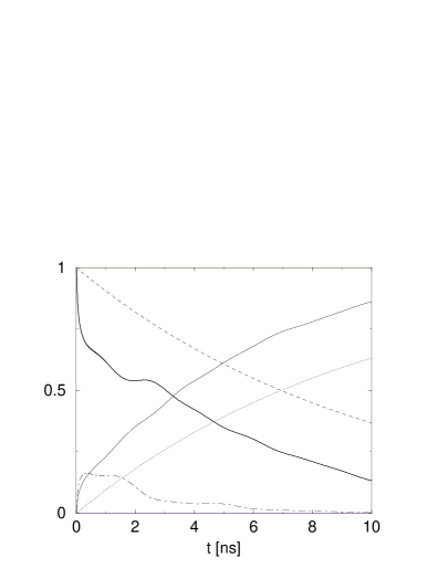
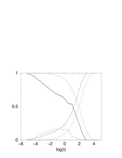
Figure 2: The ground and the first excited state population, and the leakage (the dot-dashed curve) at $T=0$. $\Omega=1[GHz]$, $\gamma=0.1[GHz]$, $\Lambda=100[GHz]$. The thick solid (dashed) curve is the exact (Markovian) result for excited states while the thin solid (dotted) curve is the exact (Markovian) result for ground states. Panel (b) is in the logarithmic time scale.

Figure 3: The excited state populations and the leakage are plotted for supra-Ohmic environment. $T=10[mK]$ in panel (a) and $T=50[mK]$ in panel (b). The thick (thin) solid curves is an exact result for supra-Ohmic (Ohmic) case, while the dashed line is from the Born-Markov approximation. $\Omega=1.5[GHz]$, $\gamma=0.1$, $\Lambda=100[GHz]$.

Figure 4: The excited state populations in the presence and absence of external field at $T=10[mK]$ are plotted for Ohmic environment in panel (a) and for supra-Ohmic environment in panel (b). The applied external is sinusoidal in the form: $E=E_{0}\cos(\Omega t)$ with $E_{0}=1.0$. The thick (thin) curves are exact results in the presence (absence) of external field, while the dashed curves are from the Born-Markov apporoximation. $\Omega=1.5[GHz]$,$\gamma=0.1$,$\Lambda=100[GHz]$.

4.2 Discussion

We saw that at low enough temperatures, many conventional approaches based on the Born-Markov approximation can significantly underestimate the environment-induced decoherence beyond the weak system-bath coupling. In this regime, the visibility in Rabi oscillations in the exact calculation tends to be lower than what is expected in the Markovian approximation. Low visibility in Rabi oscillations is commonly observed in superconducting qubits[21, 22, 23, 24]. The bath time scale is also important in causing the initial rapid decoherence and leakage; this is completely neglected in analysis based on the Born-Markov-RWA. This initial effect can manifest itself as an onset value of Rabi-oscillations. In many practical implementations of qubits, the temperature of the environment compared to the bath is small, $k_{B}T<<\hbar\Lambda$, thus we are in the low temperature regime.

The E2L-SBM approach gives a precise evaluation of the leakage due to the system’s interaction with the environment and the external control field. For temperatures higher than the characteristic energy of the oscillator, the large leakage makes the qubit based on the choice of the lowest two levels ill-defined. During gate operations, this can become a serious problem and remedies for stabilizing the system such as using external pulse control may be necessary. Our result shows that the time scale associated with leakage is characterized by the dynamical time scale of the system and the bath.

In realistic macro- or mesoscopic systems, the potential contains anharmonicity, which causes the deviation of the system dynamics from the harmonic motion. A measure of anharmonicity near ground states can be given by the ratio of energy level separation between the lowest levels $\omega_{01}\equiv\omega_{1}-\omega_{0}$ and the excited levels $\omega_{12}\equiv\omega_{2}-\omega_{1}$. When this ratio is small, $\omega_{12}/\omega_{01}<<\omega_{01}$, the initial short time evolution around a metastable state can be well-described by the linear dynamics. When the correction to the energy level due to anharmonicity in the potential becomes important, it is necessary to include such an effect in our scheme. Although the large anharmonicity also prevents the leakage in the long term, the initial large leakage we saw cannot be completely eliminated for the reason we mentioned before. When we apply our formalism to the metastable state, eventually the system state will leave the harmonic oscillator phase space into other metastable states via tunneling. The harmonic approximation of coherent dynamics is expected to be accurate at initial times when the time scales associated with these nonlinear effects are large compared to the decoherence time scale. In our example, the deviation from the Markovian prediction is evident in the very early stage of the system evolution up to $t\sim 1[ns]$ even for an intermediate temperature. For the realistic implementation of qubits, the underlying potential landscape leading to the discrete energy level is already known by design[21, 22, 23, 24, 28, 29]. Our approach based on E2L-SBM is suitable in this situation and will give a more precise estimate of the open system dynamics than the one based on the conventional 2LS approximation. In particular, our results are directly relevant to the superconducting phase qubit models [21, 22, 29]. In the superconducting qubits, the major source of decoherence is the noise induced by the interaction with the current or charge sources mainly during the qubit manipulations. We have not considered other possible sources of decoherence such as the coupling to defects or nuclear and magnetic spins. Multilevel structure in the superconducting flux qubits was studied in [30] by Born-Markov approximation without control fields.

For the system-environment coupling we considered in Eq.(11), the Fock state is not an eigenstate of the interaction Hamiltonian and is subjected to a complex decay even under the Born-Markov approximation as shown in Sec. 3.3.2. Previous study in the high temperature limit indicates the pointer state under this system-environment coupling is a coherent state[7]. Our calculation based on the exact solution for QBM indicates that, beyond the weak coupling regime, the environment-induced effect has a crucial impact on the system dynamics at an early stage. A factorized initial condition is used to derive our main results in accord with the initialization scheme used commonly in quantum information processing [31]. From the decoherence study of QBM in the presence of the initial system-bath correlation due to the preparation effect[4, 32], we expect that our results are robust and should hold for a more general class of initial conditions.

References

- [1] Decoherence and the Appearance of the Classical World in Quantum Theory, eds. D. Giulini, et al., (Springer, Berlin, 1996).
- [2] J. P. Paz and W. H. Zurek, in Coherent Matter Waves, Les Houches Lectures Session LII, (North Holland, Amsterdam, 1999).
- [3] W.G. Unruh, Phys. Rev. A51,992 (1995).
- [4] U. Weiss, Quantum Dissipative Systems, (World Scientific, Sigapore, 1999).
- [5] A. O. Caldeira and A. J. Leggett,Physica A121, 587 (1983); V. Hakim and V. Ambegaokar, Phys. Rev. A32, 423 (1985); F. Haake and R. Reibold, Phys. Rev. A32, 2462 (1985); H. Grabert, P.Schramn and G. L. Ingold, Phys. Rep. 168, 115 (1988); W. G. Unruh and W. H. Zurek, Phys. Rev. D40, 1071 (1989); B. L. Hu and Y. Zhang, Mod. Phys. Lett. A8, 3575 (1993); Int. J. Mod. Phys. A10 (1995) 4537; J. J. Halliwell and A. Zoupas, Phys. Rev. D52, 7294 (1995); C. Anastopoulos and J. J. Halliwell, Phys. Rev. D51, 6870 (1995).
- [6] B. L. Hu, J. P. Paz and Y. Zhang, Phys. Rev. D45, 2843 (1992).
- [7] W. H. Zurek, S. Habib, and J. P. Paz, Phys. Rev. Lett. 70, 1187 (1993).
- [8] A. J. Leggett, S. Chakravarty, A. T. Dorsey, M. P. A. Fisher, A. Garg, and W. Zwerger, Rev. Mod. Phys. 59, 1 (1987).
- [9] L. Tian and S. Lloyd, Phys. Rev. A 62, 050301 (2000).
- [10] Y. Nakamura, Yu. A. Pashkin, T. Yamamoto, and J.S. Tsai, Phys. Rev. Lett.88, 047901 (2002).
- [11] K. Shiokawa and D. A. Lidar, Phys. Rev. A 69, 030302 (2004); H. Gutmann, F. K. Wilhelm, W. M. Kaminsky, and S. Lloyd, cond-mat/0308107; L. Faoro and L. Viola, quant-ph/0312159; G. Falci, A. D’Arrigo, A. Mastellone, and E. Paladino,cond-mat/0312442.
- [12] W. H. Luiselle, Quantum Statistical Properties of Radiation, (Wiley, New York, 1990); H. J. Carmicheal,Statistical Methods in Quantum Optics, (Springer, Berlin, 1999).
- [13] K. Shiokawa and R. Kapral, J. Chem. Phys. 117, 7852 (2002).
- [14] R. P. Feynman and F. L. Vernon, Ann. Phys. 24, 118 (1963).
- [15] E. Wigner, Phys. Rev. 40, 749 (1932).
- [16] L. Mandel and E. Wolf, Optical Coherence and Quantum Optics, (Cambridge University Press,Cambridge,1995).
- [17] J. Twamley, Phys. Rev. D48, 5730 (1993).
- [18] C. Cohen-Tannoudiji, J. Dupont-Roc, and G. Grynberg, Atom-Photon Interactions, (Wiley, New York, 1992).
- [19] G. W. Ford and R. F. O’Connell, Physica A 243, 377 (1997).
- [20] D. Ahn, J. Lee, M. S. Kim, S. W. Hwang, Phys. Rev. A 66, 012302 (2002); D. Loss and D. P. DiVincenzo, “Exact Born Approximation for the Spin-Boson Model”, cond-mat/0304118.
- [21] Y. Yu, S. Han, X. Chu, S. I. Chu, Z. Wang, Science 296, 8898 (2002).
- [22] J. M. Martines, S. Nam, J. Aumentado, and C. Urbina, Phys. Rev. Lett. 89, 117901-1 (2002).
- [23] D. Vion, A. Aassime, A. Cottet, P.Joyez, H. Pothier, C. Urbina, D. Esteve, M. H. Devoret, Science 296, 886 (2002).
- [24] I. Chiorescu, Y. Nakamura, C. H. P. M. Harmans, J. E. Mooij, Science 299, 1869 (2003).
- [25] A. Garg and G. H. Kim, Phys. Rev. Lett. 63, 2512 (1989); P. M. V. B. Barone and A. O. Caldeira, Phys. Rev. A43, 57 (1991); S. A. Egorov and B. J. Berne, J. Chem. Phys. 107, 6050 (1997).
- [26] P. Pechukas, in Large-Scale Molecular Systems, NATO ASI series V258, (Plenum Press, New York,1991).
- [27] N. Hashitsume, F. Shibata, and M. Shingu, J. Stat. Phys. 17, 155 (1977).
- [28] Y. Makhlin, G. Schön, A. Shnirman, Rev. Mod. Phys. 73, 357 (2001).
- [29] A. J. Berkley, H. Xu, R. C. Ramos, M. A. Gubrud, F. W. Strauch, P. R. Johnson, J. R. Anderson, A. J. Dragt, C. J. Lobb, and F. C. Wellstood, Science 300, 1548 (2003).
- [30] G. Burkard, R. H. Koch, D. P. DiVincenzo, Phys. Rev. B 69, 064503 (2004).
- [31] M. A. Nielsen and I. L. Chuang, Quantum Computation and Quantum Information, (Cambridge University Press, Cambridge, 2000).
- [32] L. D. Romero, and J. P. Paz, Phys. Rev. A 55, 4070 (1997).