Entropy, entanglement, and area:
analytical results for harmonic lattice systems

Abstract

We revisit the question of the relation between entanglement, entropy, and area for harmonic lattice Hamiltonians corresponding to discrete versions of real free Klein-Gordon fields. For the ground state of the $d$-dimensional cubic harmonic lattice we establish a strict relationship between the surface area of a distinguished hypercube and the degree of entanglement between the hypercube and the rest of the lattice analytically, without resorting to numerical means. We outline extensions of these results to longer ranged interactions, finite temperatures and for classical correlations in classical harmonic lattice systems. These findings further suggest that the tools of quantum information science may help in establishing results in quantum field theory that were previously less accessible.

Imagine a distinguished geometrical region of a discretized free quantum Klein-Gordon field: what is the entropy associated with a pure state obtained by tracing over the field variables outside the region? How does this entropy relate to properties of the region, such as volume and boundary area? This innocent-looking question is a long-standing issue indeed, studied in the literature under the key word of geometric entropy. Analytical steps supplemented by numerical computations for half-spaces and spherical configurations in seminal works by Bombelli et al. Bombelli KLS 86 and Srednicki Srednicki 93 strongly suggested a direct connection between entropy and area. The interest in this quantity for quantum field theory is drawn from the fact that geometric entropy is thought to be the leading quantum correction to the Bekenstein-Hawking black hole entropy BlackHoleStuff . Subsequent work employed various approaches, such as methods from conformal field theory Holzhey 95 , analysis of entropy subadditivity Casini 04 or mode counting Yurtsever 03 . Recently, there has been renewed interest in studying entanglement and correlations in quantum many-body systems and quantum field theory, largely due to availability of novel powerful methods from the quantitative theory of entanglement in the context of quantum information theory Stelmachovic B 01 ; Summers W 85 ; Audenaert EPW 02 ; Fannes HM 03 ; Wolf VC 04 ; Botero R 04 ; Latorre . Such ideas have previously been employed to assess the entanglement in settings of one-dimensional spin (see, e.g., Refs. Fannes HM 03 ; Latorre ) and harmonic chains Audenaert EPW 02 ; Botero R 04 .

This letter gives an analytical answer to the question of the scaling of the degree of entanglement for harmonic lattice Hamiltonians such as discrete versions of the free scalar Klein-Gordon field, in arbitrary spatial dimensions. Although we encounter a highly correlated system we nevertheless find an ‘area-dependence’ of the degree of entanglement. Our analysis is based on methods that have been developed in recent years in quantum information theory, in particular those relating to entanglement in Gaussian (quasi-free) states (see, e.g., Ref. Eisert P 03 ). These methods allow us to give an analytical answer to the question of the scaling of the degree of entanglement between a region and its exterior for harmonic lattice Hamiltonians such as discrete versions of the free scalar Klein-Gordon field, in arbitrary spatial dimensions. It is remarkable that although we encounter a highly correlated system, we nevertheless find an ”area dependence” of the degree of entanglement.

The Hamiltonian. — The starting point of the argument is a discrete lattice version of a free real scalar quantum field. For any $d\geq 1$ we consider a $d$-dimensional simple cubic lattice $n^{\times d}$ comprising $n^{d}$ oscillators. We may write the Hamiltonian as

$$H=\mathbf{p}\mathbf{p}^{\text{T}}/2+\mathbf{x}V\mathbf{x}^{\text{T}}/2,$$ (1)

where $\mathbf{x}=(x_{1},\dots,x_{n^{d}})$ and $\mathbf{p}=(p_{1},\dots,p_{n^{d}})$ denote the canonical coordinates of the system. The $n^{d}\times n^{d}$-matrix $V$, the potential matrix, specifies the coupling between the oscillators in the position coordinates.

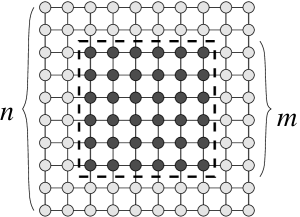
Figure 1: The harmonic lattice in $d=2$ with a distinguished $m\times m$ region in an $n\times n$ lattice.

For now $V$ will be chosen such that in the continuum limit one obtains the Hamiltonian of the real Klein-Gordon field, under periodic boundary conditions. We will therefore consider the harmonic lattice Hamiltonian with nearest-neighbor interaction. Note that our argument can be extended to other types of interactions. The case of next-to-nearest-neighbor coupling will also be discussed later in this paper, see Ref. Long for a more general discussion.

We write $V=\operatorname{circ}(\mathbf{v})$ for the circulant matrix whose first row is given by the $n$-tupel $\mathbf{v}$, and also for a block circulant matrix where the first block column is specified by a tupel of matrices. So in $d=1$, we have $V_{1}=\operatorname{circ}(1,-c,0,\dots,0,-c)$ and in higher dimensions we have a recursive, block-circulant structure reflecting rows, layers etc.:

$$V_{d}=\operatorname{circ}(V_{d-1},-c\mathbbm{1}_{n^{d-1}},0,\dots,0,-c\mathbbm{1}_{n^{d-1}})$$

with a $0\leq 2cd<1$. From now on we will write $V$ instead of $V_{d}$.

Entanglement and area dependence. — We denote the ground state of the system by $\rho$. For a distinguished cubic region $m^{\times d}$ in a lattice $n^{\times d}$ (see Fig. 1) its entropy of entanglement is

$$E_{n,m}=-\operatorname{tr}\rho_{n,m}\log\rho_{n,m}.$$

The reduced density matrix $\rho_{n,m}$ is formed by tracing out the variables outside the region $m^{\times d}$. We will show the following:

The entropy of entanglement of the distinguished region $m^{\times d}$ in the lattice $n^{\times d}$ satisfies

$$\lim_{n\rightarrow\infty}E_{n,m}=\Theta(m^{d-1}),$$ (2)

where $\Theta$ is the Landau-theta. More specifically, we have that $C_{1}\,m^{d-1}\leq E_{n,m}\leq C_{2}\,m^{d-1}$ for sufficiently large $m$, with appropriate $C_{1},C_{2}>0$.

The ‘area dependence’ manifests itself as follows: For a linear chain, the entropy of entanglement is bounded by quantities that are independent of the size of the distinguished interval. In two dimensions, this dependence is linear in the length of the boundary, in three dimensions to the area of the boundary. Indeed, one can show that while all oscillators are correlated with all oscillators, the correlations over the boundary decay very quickly. In effect, for fixed interaction strength , the only significant contribution comes from within a finite width, the correlation length, along the boundary, and thus leads to a surface dependence of the correlations. This intuition forms the basis of the following, fully analytical argument, where the above statement is proven by finding upper and lower bounds for which the statement holds.

The upper bound. — The ground state $\rho$ of the coupled harmonic system in Eq. (1) is a Gaussian (quasi-free) state with vanishing first moments. The second moments of $\rho$ can be collected in the covariance matrix $\gamma$, which is defined as $\gamma_{j,k}=2\text{Re}[R_{j}R_{k}\rho]$ for $j,k=1,\dots,2n^{d}$, where $\mathbf{R}=(x_{1},\dots,x_{n^{d}},p_{1},\dots,p_{n^{d}})$ is the vector of canonical coordinates. In terms of the potential matrix $V$ the covariance matrix of the ground state is then found to be $\gamma=V^{-1/2}\oplus V^{1/2}$ Audenaert EPW 02 . From entanglement theory we know that an upper bound for the entropy of entanglement is provided by the logarithmic negativity $E_{N}=\ln\lVert\rho^{\Gamma}\rVert_{\text{tr}}$, where $\rho^{\Gamma}$ is the partial transpose of $\rho$, and $\lVert\cdot\rVert_{\text{tr}}$ denotes the trace norm Neg . Following Ref. Audenaert EPW 02 we find

$$E_{N}=\sum_{j=1}^{n^{d}}\ln(1+\max(0,\lambda_{j}(Q-\mathbbm{1}))),$$ (3)

where $\lambda_{j}(Q)$ are the non-increasingly ordered eigenvalues of the matrix

$$Q=V^{-1/2}PV^{1/2}P.$$ (4)

In a reordered list of canonical coordinates (such that the inner oscillators are counted first) $P$ is the diagonal matrix $P=-\mathbbm{1}_{m^{d}}\otimes\mathbbm{1}_{n^{d}-m^{d}}$ and the potential matrices can be written as

$$V^{-1/2}=\begin{bmatrix}A&B\\ B^{\text{T}}&C\end{bmatrix},\,V^{1/2}=\begin{bmatrix}D&E\\ E^{\text{T}}&F\end{bmatrix},\,T=\begin{bmatrix}0&E\\ E^{\text{T}}&0\end{bmatrix}.$$

The matrices $B$ and $E$ describe the couplings between the $m^{d}$ oscillators forming the distinguished hypercube and the rest of the lattice. On using $V^{-1/2}V^{1/2}=\mathbbm{1}$, we arrive at

$$Q-\mathbbm{1}=-2V^{-1/2}T$$

This is convenient as it will turn out that the detailed structure of $V^{-1/2}$ will not have to be considered and we can concentrate on the properties of the matrix $T$. To avoid taking the maximum in Eq. (3) we bound the eigenvalues by their absolute values,

$$E_{N} \leq\sum_{j=1}^{n^{d}}\ln(1+|\lambda_{j}(Q-\mathbbm{1})|)$$

$$\leq\sum_{j=1}^{n^{d}}|\lambda_{j}(Q-\mathbbm{1})|=\lVert Q-\mathbbm{1}\rVert_{\text{tr}},$$

where we have employed that $\ln(1+x)\leq x$ for all $x\geq 0$. Since the trace norm is unitarily invariant Matrix , we may further write

$$\lVert Q-\mathbbm{1}\rVert_{\text{tr}}=2\ \lVert V^{-1/2}T\rVert_{\text{tr}}\leq 2\ \lambda_{1}(V^{-1/2})\ \lVert T\rVert_{\text{tr}}.$$

Here we also have that $V^{-1/2}$ is symmetric. The spectrum of $V$ can be obtained via discrete Fourier transform and yields $\lambda_{1}(V^{-1/2})=(1-2cd)^{-1/2}$.

Now the trace norm of $T$ can be bounded from above by the sum of the absolute values of all the matrix elements of $T$, which is known as the $l_{1}$ matrix norm Matrix . Therefore,

$$E_{N}\leq\frac{2}{\sqrt{1-2cd}}\sum_{i,j=1}^{n^{d}}\lvert T_{ij}\rvert.$$

In the following we will bound the matrix elements of $V^{1/2}$ and consequently those of $T$. The explicit implementation of the multidimensional discrete Fourier transform is non-technical yet involved. To achieve a more compact notation, we introduce the lattice coordinate vectors $\mathbf{k},\mathbf{l}$ where $k_{j},l_{j}=0,\dots,n-1$ and $j=0,\dots,d-1$. For the considered lattice structure we may write $V_{\mathbf{k},\mathbf{l}}=V_{\sum_{j=0}^{d-1}k_{j}n^{j},\sum_{j=0}^{d-1}l_{j}n^{j}}$ for the interaction term between site $\mathbf{k}$ and $\mathbf{l}$. The matrix elements of $V^{1/2}$ are then given by

$$V^{1/2}_{\mathbf{k},\mathbf{l}} = \sum_{\mathbf{k}^{\prime}}\prod_{j=0}^{d-1}\frac{e^{2\pi ik^{\prime}_{j}(k_{j}-l_{j})/n}}{n^{d}}\biggl{(}1-2c\sum_{r=0}^{d-1}\cos\frac{2\pi k_{r}^{\prime}}{n}\biggr{)}^{1/2}.$$

To bound these, we replace the square root by its power series expansion in the parameter $2c$. This converges if $2cd\leq 1$, which coincides with the constraint imposed by the positivity of the potential matrix. We will use $(1-x)^{1/2}=-\sum_{s=1}^{\infty}B_{s}x^{s}$, with $0<B_{s}<1$ and the fact that $\sum_{q=1}^{n}e^{{2\pi ipq}/{n}}=0$ for integer $p$ and $q$ unless $p$ is a multiple of $n$. With this the non-diagonal elements of $V^{1/2}$, and analogously $V^{-1/2}$, are bounded by

$$\frac{y^{s(\mathbf{k},\mathbf{l})}}{1-y}\geq V^{-1/2}_{\mathbf{k},\mathbf{l}}\geq 0\geq V^{1/2}_{\mathbf{k},\mathbf{l}}\geq- \frac{y^{s(\mathbf{k},\mathbf{l})}}{1-y},$$ (5)

where $s(\mathbf{k},\mathbf{l})=(k_{0}-l_{0})+\dots+(k_{n-1}-l_{n-1})$, $y=2cd$ and $0\leq k_{j}-l_{j}\leq n/2$. This demonstrates the exponential decay of the off-diagonal elements in these block circulant matrices. The remaining matrix elements are determined by the periodic boundary conditions under the exchange $k_{j}-l_{j}\mapsto n-(k_{j}-l_{j})$. Note that generally $s(\mathbf{k},\mathbf{l})$ is simply the number of lattice steps one has to make starting at site $\mathbf{k}$ to reach site $\mathbf{l}$. If, for example, $s(\mathbf{k},\mathbf{l})=1$ then the oscillators are direct neighbors.

We may now proceed with the computation of the $l_{1}$ norm of $T$, i.e., of the blocks in $V^{1/2}$ that describe the coupling between the distinguished region and the rest of the lattice. Given that the region is a hypercube, this can be done in a transparent way. Consider the set ${\cal L}_{0}$ of $m^{d}-(m-2)^{d}$ oscillators of the hypercube that lie directly on the boundary and successively the sets ${\cal L}_{r}$ of $(m-2r)^{d}-(m-2r-2)^{d}$ oscillators inside that are exactly $r$ steps away from the surface of the hypercube. Starting from the set ${\cal L}_{0}$ and taking $s$ steps on the lattice one can reach less than $(m+2s)^{d}-m^{d}$ oscillators outside the hypercube $m^{\times d}$. Therefore we find that the sum of all the elements of $T$ that couple oscillators from the set ${\cal L}_{0}$ to oscillators outside the hypercube is bounded by

$$S_{0}\leq 2\sum_{s=1}^{\infty}((m+2s)^{d}-m^{d})\frac{y^{s}}{1-y}\,.$$

Now consider the contribution from the set ${\cal L}_{k}$. Clearly, any oscillator outside the hypercube that can be reached from ${\cal L}_{k}$ in $s+k$ steps can be reached from ${\cal L}_{0}$ in $s$ steps. Therefore we can bound the sum $S_{k}$ of all the elements of $T$ that couple the set ${\cal L}_{k}$ to oscillators outside the hypercube by

$$S_{k} \leq 2\sum_{s=k+1}^{\infty}((m+2(s-k))^{d}-m^{d})\frac{y^{s}}{1-y}.$$

As a consequence we obtain

$$E_{N} \leq \frac{2}{\sqrt{1-2cd}}\sum_{k=0}^{m/2}S_{k}$$

$$\leq \frac{2}{\sqrt{1-2cd}}\sum_{s=1}^{\infty}((m+2s)^{d}-m^{d})\frac{y^{s}}{1-y}\sum_{k=0}^{m/2}y^{k}.$$

Using the binomial expansion of $(m+2s)^{d}$ and the Gamma-function to bound expressions of the form $\sum_{s=0}^{\infty}y^{s}(2s)^{k}$ we find for $m>4d/|\ln(y)|$ the bound

$$E_{N} \leq \frac{16d}{\sqrt{1-2cd}(1-2cd)^{2}|\ln(1-2cd)|^{2}}\,m^{d-1},$$ (6)

which is the desired upper bound that is linear in the number of oscillators on the surface of the hypercube.

Lower bound. — In the following we demonstrate that the degree of entanglement, measured by the entropy of entanglement, is asymptotically at least linear in the number of oscillators. The entropy of entanglement depends only on the symplectic spectrum of the covariance matrix $\gamma_{A}$ corresponding to the reduced Gaussian state of the interior. The non-increasingly ordered symplectic eigenvalues satisfy $\mu_{i}=(\lambda_{i}(AD))^{1/2}\geq 1$ from which the entropy of entanglement can be evaluated as

$$S = \sum_{i=1}^{m^{d}}\left(\frac{\mu_{i}+1}{2}\log\frac{\mu_{i}+1}{2}-\frac{\mu_{i}-1}{2}\log\frac{\mu_{i}-1}{2}\right).$$

For $\mu_{i}>1$ each bracketed terms in the sum can be bounded from below by $\log\mu_{i}$. Because $\mu_{i}\leq\left((1+2c)/(1-2c)\right)^{1/4}$ for all $i$, we find

$$S\geq\sum_{i=1}^{m^{d}}\log\left(1+\left(\mu_{i}-1\right)\right)\geq\frac{\log\mu_{1}}{\mu_{1}-1}\sum_{i=1}^{m^{d}}\left(\mu_{i}-1\right)\,.$$

Employing that for $\beta=(\sqrt{1+k}-1)/k$ we have $\sqrt{1+x}\geq 1+\beta x$ in $x\in[0,k]$ and $\lambda_{i}(AD)=1+\lambda_{i}(-BE^{\text{T}})$ we find

$$S\geq\frac{\sqrt{1+\lambda_{1}(-BE^{\text{T}})}-1}{\lambda_{1}\left(-BE^{\text{T}}\right)}\frac{\log\mu_{1}}{\mu_{1}-1}\operatorname{tr}\left(-BE^{\text{T}}\right).$$

The factors in front of the trace can be bounded from above by a quantity that is independent of both $m$ and $n$. All the elements of $V^{-1/2}$ and of $-E$ are positive. Using the techniques that led to Eqs. (5)) we find

$$\lvert V^{\pm 1/2}_{\mathbf{k},\mathbf{l}}\rvert \geq \frac{1}{2}\left(\frac{c}{2}\right)^{s(\mathbf{k},\mathbf{l})}\frac{1}{1-c^{2}}\,.$$

As a consequence we have

$$\operatorname{tr}\left(-BE^{\text{T}}\right)\geq\sum_{\mathbf{k},\mathbf{l}}\left(\frac{1}{2}\left(\frac{c}{2}\right)^{s(\mathbf{k},\mathbf{l})}\frac{1}{1-c^{2}}\right)^{2}\,.$$

Now we employ counting methods analogous to those used in the derivation for the upper bound we find an expression linear in the area. We take into account only contributions to the above sum that correspond to the $2dm^{d-1}$ oscillators that can be reached in each step moving outwards orthogonal to the surface of the hypercube. We thus obtain a lower bound proportional to the surface of the hypercube $m^{\times d}$ for $m>m_{0}$ and appropriate $m_{0}$. This concludes the proof.

In the following we will briefly describe possible extensions of the above results that can be obtained by similar techniques, including more general interactions, thermal states and classical correlations in classical systems.

‘Squared interactions’. — The basic intuition behind the entanglement-area dependence becomes most transparent for the specific class of interactions for which the potential matrices $V$ is of the form $V=W^{2}$ with a circulant band-matrix $W$. In that case the covariance matrix of the ground state is given by $\gamma=W^{-1}\oplus W$. In this case one arrives at Eq. (2) since one can show that (i) the number of terms contributing to the symplectic spectrum of the reduced covariance matrix is linear in the number of degrees of freedom at the boundary of the region, and (ii) the respective symplectic eigenvalues are bounded from above and below independently of $n$ and $m$. Note that property (i) is equivalent to the existence of a ‘disentangling’ symplectic unitary transformation local to inside and outside of the regions such that only oscillators near to the boundary remain entangled. Taking e.g. $V_{1}=\operatorname{circ}(1+2c^{2},-2c,c^{2},0,\dots,0,c^{2},-2c)$ – the case of nearest-neighbor and smaller next-to-nearest-neighbor interactions – allows to show that only the oscillators exactly at the boundary contribute to the logarithmic negativity and that $\lambda_{1}(Q)\leq 2/(1-2c)-1$, with $Q$ being defined as in Eq. (4). For the same interaction in $d=1$ spatial dimension one can even exactly calculate the symplectic spectrum of the reduced covariance matrix by means of a simple recursion relation. In the limit $m\rightarrow\infty$ this results in the two non-vanishing symplectic eigenvalues $\mu_{1}=\mu_{2}=(1-c^{2}/q^{2})^{-1/2}$, where $q=c+1/2\pm(c+1/4)^{1/2}$.

Entanglement and area in classical systems. — It should be noted that, perhaps surprisingly, an ‘area-dependence’ can also be established analytically for classical correlations in classical harmonic lattice systems Long . It is noteworthy that this result on classical systems can be established most economically using quantum techniques namely, mapping the problem onto that of a quantum harmonic lattice with a squared interaction as has been described above.

Entanglement and area at finite temperature. — The property of squared interactions leading to effective disentanglement extends to thermal states and therefore permits the proof of the linear entanglement–area dependence for finite temperatures. In that case operational entanglement measures such as the distillable entanglement have to be used. They can be bounded from below by the hashing inequality and above again by the logarithmic negativity Long .

Summary and outlook. — For certain harmonic lattice Hamiltonians, e.g. discrete versions of the real Klein-Gordon field, we have proven analytically that the degree of entanglement between a hypercube and its environment can be bounded from above and below by expressions proportional to the number of degrees of freedom on the surface of the hypercube . This establishes rigorously a connection between entanglement and area in this system. Intuitively, this originates from the fact that one can approximately decouple the oscillators in the interior and the exterior up to a band of the width of the order of the correlation length of the system, which can be, as outlined for the case of next-to-nearest neighbor coupling, equal to just one lattice unit.

Our results can be extended to a wide variety of harmonic lattice Hamiltonians, both quantum and classical, and a future publication Long will present details for more general interactions, both ground and thermal states and a careful discussion of the continuum limit, where the effective interaction strength is modified. These results in particular rely in an essential way on the insights and techniques that have been obtained in recent years in the development of a quantitative theory of entanglement in quantum information science.

Acknowledgements. — We warmly thank K. Audenaert for input at earlier stages of this project, and J. Oppenheim, T. Rudolph and R. F. Werner for discussions. We would also like to thank J. I. Latorre and G. Vidal for bringing the related Ref. Calabrese C 04 to our attention. This work was supported by the DFG (SPP 1078), the EU (IST-2001-38877), the EPSRC (QIP-IRC), and a Royal Society Leverhulme Trust Senior Research Fellowship.

References

- (1) L. Bombelli, R. K. Koul, J. Lee, and R. D. Sorkin, Phys. Rev. D 34, 373 (1986).
- (2) M. Srednicki, Phys. Rev. Lett. 71, 666 (1993).
- (3) J. M. Bardeen, B. Carter and S. W. Hawking, Commun. Math. Phys. 31, 161 (1973); J. D. Bekenstein, Lett. Nuovo Cimento 4, 737 (1972); G. ’t Hooft, Nucl. Phys. B 256, 727 (1985); J. D. Bekenstein, Contemp. Phys. 45, 31 (2004); D. Kabat and M. J. Strassler, Phys. Lett. B 329, 46 (1994); T. M. Fiola, J. Preskill, A. Strominger, and S. P. Trivedi, Phys. Rev. D 50, 3987 (1994); G. Gour and A. E. Mayo, ibid. 63, 064005 (2001). C. Callan and F. Wilczek, Phys. Lett. B 333, 55 (1994).
- (4) C. Holzhey, F. Larsen and F. Wilczek, Nucl. Phys. B 424, 443 (1995).
- (5) H. Casini, Class. Quant. Grav. 21, 2351 (2004).
- (6) U. Yurtsever, Phys. Rev. Lett. 91, 041302 (2003).
- (7) P. Stelmachovic and V. Buzek, presented at a quantum information conference in Gdansk (July 2001); P. Stelmachovic and V. Buzek, Phys. Rev. A 70, 032313 (2004).
- (8) S. J. Summers and R. F. Werner, Phys. Lett. A 110, 257 (1985); H. Halvorson and R. Clifton, J. Math. Phys. 41, 1711 (2000); R. Verch and R. F. Werner, quant-ph/0403098; B. Reznik, A. Retzker, and J. Silman, quant-ph/0310058; B. Reznik, A. Retzker and J. Silman, J. Mod. Opt. 51, 833 (2004).
- (9) K. Audenaert, J. Eisert, M. B. Plenio, and R. F. Werner, Phys. Rev. A 66, 042327 (2002).
- (10) M. M. Wolf, F. Verstraete, and J. I. Cirac, Phys. Rev. Lett. 92, 087903 (2004).
- (11) A. Botero and B. Reznik, Phys. Rev. A 70, 052329 (2004).
- (12) M. Fannes, B. Haegeman, and M. Mosonyi, J. Math. Phys. 44, 6005 (2003).
- (13) G. Vidal, J. I. Latorre, E. Rico, and A. Kitaev, Phys. Rev. Lett. 90 227902 (2003); J. I. Latorre, E. Rico, and G. Vidal, Quant. Inf. Comp. 4, 48 (2004); J. I. Latorre, C. A. Lutken, G. Vidal, quant-ph/0404120.
- (14) J. Eisert and M. B. Plenio, Int. J. Quant. Inf. 1, 479 (2003).
- (15) J. Eisert and M. B. Plenio, J. Mod. Opt. 46, 145 (1999); J. Eisert (PhD thesis, Potsdam, February 2001); G. Vidal and R. F. Werner, Phys. Rev. A 65, 032314 (2002); K. Audenaert, M. B. Plenio, and J. Eisert, Phys. Rev. Lett. 90, 027901 (2003).
- (16) R. A. Horn and C. R. Johnson, Matrix Analysis (Cambridge University Press, Cambridge, 1985).
- (17) Forthcoming publication by the same authors in different order.
- (18) P. Calabrese and J. Cardy, J. Stat. Mech. Th. Exp P00406 (2004).