Lindblad and non–Lindblad type dynamics of a quantum Brownian particle

Abstract

The dynamics of a typical open quantum system, namely a quantum Brownian particle in a harmonic potential, is studied focussing on its non-Markovian regime. Both an analytic approach and a stochastic wave function approach are used to describe the exact time evolution of the system. The border between two very different dynamical regimes, the Lindblad and non-Lindblad regimes, is identified and the relevant physical variables governing the passage from one regime to the other are singled out. The non-Markovian short time dynamics is studied in detail by looking at the mean energy, the squeezing, the Mandel parameter and the Wigner function of the system.

I Introduction

The description of the dynamics of quantum systems interacting with their surrounding is, in general, a very difficult task due to the complexity of the environment. An exact approach would require to take into account not only the degrees of freedom of the system of interest, but also those of the environment. One can, in principle, look for the solution of the Liouville - von Neumann equation for the density matrix of the total closed system. Even when this is possible, however, the total density matrix contains much more information than what we actually need, since one is usually interested in the time evolution of the reduced system only.

A common approach to the dynamics of open quantum systems consists in deriving a master equation for the reduced density matrix describing the temporal behavior of the open system petruccionebook . This equation is in general obtained by tracing over the environmental variables, after performing a series of approximations. Two of the most common ones are the Rotating Wave Approximation (RWA) and the Born-Markov approximation. The first one basically consists in neglecting in the microscopic system-reservoir interaction Hamiltonian the counter-rotating terms responsible for the virtual exchanges of energy between system and environment. The second one neglects the correlations between system and reservoir assuming that the changes in the reservoir due to the interaction with the system cannot feed back into the system’s dynamics.

The Born-Markov approximation leads to a master equation which can be cast in the so called Lindblad form Lindblad ; Gorini . Master equations in the Lindblad form are characterized by the fact that the dynamical group of the system satisfies both the semigroup property and the complete positivity condition, thus ensuring the preservation of positivity of the density matrix during the time evolution. Moreover, it has been shown that numerical techniques as the Monte Carlo Wave Function method can always, in principle, be applied to the description of the dynamics, provided that the master equation is in the Lindblad form Molmer96a .

In many solid state systems such as photonic band gap materials and quantum dots the Markov approximation is, however, not justified quang97 . Similarly, the reservoir interacting with a single mode cavity in atom lasers is strongly non-Markovian hope00 . These physical systems therefore necessitate non-Markovian analytical or numerical approaches to their dynamics. Moreover, the non-Markovian features become of importance when one is interested in the initial temporal regime, even for Markovian systems, where the memory time of the reservoir $\tau_{R}$ is much smaller than the system characteristic time scale $\tau_{S}$.

It is worth mentioning that during the last few years the interest in open quantum systems has increased mainly due to three reasons. On the one hand, the phenomena of decoherence and dissipation, characterizing the dynamics of a quantum system interacting with its surrounding giulini , are considered nowadays the major obstacles to the realization of quantum computers and other quantum devices nielsen . On the other hand recent experiments on engineering of environments engineerNIST pave the way to new proposals aimed at creating entanglement and superpositions of quantum states exploiting decoherence and dissipation cirac ; plenio . Moreover, we emphasize that presently the fields of quantum information and open quantum systems actually merge in the question to what extent the entangling power of the system-reservoir interaction is the responsible factor for decoherence plenio2 ; dodd . In order to understand deeply the origin, essence and effects of decoherence phenomena, it is of great importance to have the tools for an exact description of the open system dynamics.

In this paper we focus on an ubiquitous model of the theory of open quantum systems, that is the quantum Brownian motion model, which is also known as the damped harmonic oscillator petruccionebook ; Haake ; annals ; Feynman ; Caldeira ; Hu ; Ford ; Grabert ; PRAsolanalitica ; letteranostra ; EPJRWA ; misbelief . We consider the exact generalized master equation obtained with the time-convolutionless projection operator technique petruccionebook . We exploit an analytic approach based on the algebraic properties of the superoperators appearing in the master equation PRAsolanalitica . The knowledge of the explicit expression of the exact analytic solution of this equation allows us to study in a complete way the dynamics and, in particular, the short time non-Markovian regime. The analytic results are in very good agreement with the numerical simulations obtained by means of the non-Markovian Wave Function (NMWF) method Breuer99a , a variant of the Monte Carlo (MC) methods Dalibard92a ; Molmer93a ; Molmer96a ; Plenio98a ; Breuer04a . By looking at the dissipation and diffusion coefficients we single out those parameters governing the passage from Lindblad to non-Lindblad type regimes. The dynamics of the system in the Lindblad type regime is governed by a Lindblad type master equation, whereas in the non-Lindblad type regime, the master equation cannot be cast in the Lindblad form and the dynamics is dominated by virtual exchanges of energy between the system and the environment.

The paper is structured as follows. In Sec. II we recall the exact time-convolutionless master equation for quantum Brownian motion and its superoperatorial solution. In Sec. III we apply the non-Markovian Wave Function method to the system under scrutiny. Sections IV and V contain the main results of the paper. In Sec. IV we study the border between Lindblad and non-Lindblad regions, and in Sec. V we focus on the non-Lindblad type dynamics looking at the temporal evolution of the squeezing, of the Mandel parameter and of the Wigner function. Finally, Sec. VI concludes the paper.

II Exact dynamics of quantum Brownian particle

In this section we first recall the microscopic model and the exact master equation for the reduced density matrix of a quantum Brownian particle. Then we briefly sketch an analytic approach to derive an exact solution for the master equation.

Let us consider a harmonic oscillator of frequency $\omega_{0}$ surrounded by a generic bosonic environment. The Hamiltonian $H$ of the total system can be written as follows

$$H=H_{0}+H_{E}+\alpha XE,$$ (1)

where $H_{0}=\omega_{0}\left(P^{2}+X^{2}\right)/2$, $H_{E}$ and $\alpha XE$ are the system, environment and interaction Hamiltonians, respectively, and $\alpha$ is the dimensionless coupling constant. The interaction Hamiltonian considered here has a simple bilinear form with position of the oscillator $X$ and position environmental operator $E\equiv\sum_{n}\kappa_{n}x_{n}$, where $x_{n}$ are the position operators of the environmental oscillators. For the sake of simplicity we have written the previous expressions in terms of dimensionless position and momentum operators for the system oscillator. The key quantity governing the nature of the coupling is the spectral density $J(\omega)=\sum_{n}\kappa_{n}\delta(\omega-\omega_{n})/(2m_{n}\omega_{n})$, with $m_{n}$ and $\omega_{n}$ masses and frequencies of the environmental oscillators, respectively.

We denote by $\rho$ the density matrix of the total system. Under the assumptions that: (i) at $t=0$ system and environment are uncorrelated, that is $\rho(0)=\rho_{S}(0)\otimes\rho_{E}(0)$, with $\rho_{S}$ and $\rho_{E}$ density matrices of the system and the environment respectively; (ii) the environment is stationary, that is $[H_{E},\rho_{E}(0)]=0$; (iii) the expectation value of the environmental operator $E$ is zero, that is ${\rm Tr_{E}}\left\{E\rho_{E}(0)\right\}=0$ (as for example in the case of a thermal reservoir), one can derive the following master equation EPJRWA

$$\frac{d\rho_{S}(t)}{dt}=\frac{1}{i\hbar}\mathbf{H}_{0}^{S}\rho_{S}(t)-\Big{[}\Delta(t)(\mathbf{X}^{S})^{2}-\Pi(t)\mathbf{X}^{S}\mathbf{P}^{S}$$

$$-\frac{i}{2}r(t)(\mathbf{X^{2}})^{S}+i\gamma(t)\mathbf{X}^{S}\mathbf{P}^{\Sigma}\Big{]}\rho_{S}(t).$$ (2)

We indicate with $\mathbf{X}^{S(\Sigma)}$ and $\mathbf{P}^{S(\Sigma)}$ the commutator (anticommutator) position and momentum superoperators respectively and with $\mathbf{H}_{0}^{S}$ the commutator superoperator relative to the system Hamiltonian. It is not difficult to prove that such a master equation, obtained by using the time-convolutionless projection operator technique petruccionebook ; annals ; timeconv , is the superoperatorial version of the Hu-Paz-Zhang master equation Hu . This equation can be solved in generality Haake ; Hu ; Ford ; Grabert ; PRAsolanalitica although the time dependent coefficients have no obvious closed form. For this reason, the exact study of the non-Markovian behaviour of the system for strong couplings may be performed only by means of numerical methods. Also in this case, however, one needs, firstly, to find out the parameter regime in which a perturbation expansion to a given order yields reliable numerical results. This is in general a very difficult task. In the following we will focus on the dynamics of the system in the weak coupling limit, and in particular we will consider the case in which a truncation of the expansion in the coupling strength $\alpha$ to the second order is physically meaningful. Under this condition the time dependent coefficients appearing in the master equation can be written as follows

$$\Delta(t) = \int_{0}^{t}\kappa(\tau)\cos(\omega_{0}\tau)d\tau,$$ (3)

$$\gamma(t) = \int_{0}^{t}\mu(\tau)\sin(\omega_{0}\tau)d\tau,$$ (4)

$$\Pi(t) = \int_{0}^{t}\kappa(\tau)\sin(\omega_{0}\tau)d\tau,$$ (5)

$$r(t) = 2\int_{0}^{t}\mu(\tau)\cos(\omega_{0}\tau)d\tau,$$ (6)

where

$$\kappa(\tau)=\alpha^{2}\langle\{E(\tau),E(0)\}\rangle,$$ (7)

and

$$\mu(\tau)=i\alpha^{2}\langle[E(\tau),E(0)]\rangle,$$ (8)

are the noise and dissipation kernels, respectively. For the case of an Ohmic reservoir spectral density with Lorentz-Drude cutoff petruccionebook

$$J(\omega)=\frac{2\omega}{\pi}\ \frac{\omega_{c}^{2}}{\omega_{c}^{2}+\omega^{2}},$$ (9)

the noise and dissipation kernels assume the form

$$\kappa(\tau) = 4\alpha^{2}kT\omega_{c}^{2}\sum_{n=-\infty}^{\infty}\frac{\omega_{c}e^{-\omega_{c}\tau}-\nu_{n}e^{-|\nu_{n}|\tau}}{\omega_{c}^{2}-\nu_{n}^{2}},$$ (10)

$$\mu(\tau) = 2\alpha^{2}\omega_{c}^{2}e^{-\omega_{c}\tau},$$ (11)

where $\omega_{c}$ is the cutoff frequency and $\nu_{n}=2\pi nkT$ denote the Matsubara frequencies.

It is worth noting that, as shown in Ref. annals , it is possible to estimate in an easy way the order of magnitude of the error associated to the truncated expression of the coefficients. This allows to check the range of validity of the weak coupling approximation. The errors of the time dependent coefficients, up to the fourth order in the coupling constant, are studied in Refs. petruccionebook ; annals .

As we will see in the following, truncating the perturbation expansion to the second order, it is possible to find a closed analytic form for two time dependent coefficients playing a special role in the dynamics: the diffusion coefficient $\Delta(t)$ and the dissipation coefficient $\gamma(t)$. Dealing with a closed analytic expression of these parameters allows to gain new insight in the dynamics of the open system. In fact, the possibility of studying analytically the border between Lindblad and non-Lindblad-type dynamics stems from the availability of a closed expression for these time dependent parameters.

Let us now look in more detail at the form of the master equation (2). First of all, we note that this master equation is local in time, even if non-Markovian. This feature is typical of all the generalized master equations derived by using the time-convolutionless projection operator technique petruccionebook ; Breuer99a or equivalent approaches such as the superoperatorial one EPJRWA ; royer .

The time dependent coefficients appearing in (2) contain all the information about the short time system-reservoir correlation. The coefficient $r(t)$ gives rise to a time dependent renormalization of the frequency of the oscillator. In the weak coupling limit one can show that $r(t)$ gives a negligible contribution as far as the reservoir cutoff frequency remains finite petruccionebook . The term proportional to $\gamma(t)$ is a classical damping term while the coefficients $\Delta(t)$ and $\Pi(t)$ are diffusive terms. Averaging over the rapidly oscillating terms appearing in the time dependent coefficients of Eq.(2) one gets the following secular approximated master equation

$$\frac{d\rho_{S}}{dt}=\!\! - \!\!\!\frac{\Delta(t)+\gamma(t)}{2}\left[a^{{\dagger}}a\rho_{S}-2a\rho_{S}a^{{\dagger}}+\rho_{S}a^{{\dagger}}a\right]$$ (12)

$$- \!\!\!\frac{\Delta(t)-\gamma(t)}{2}\left[aa^{{\dagger}}\rho_{S}-2a^{{\dagger}}\rho_{S}a+\rho_{S}aa^{{\dagger}}\right]\!\!,$$

where we have introduced the bosonic annihilation and creation operators $a=\left(X+iP\right)/\sqrt{2}$ and $a^{{\dagger}}=\left(X-iP\right)/\sqrt{2}$. The form of Eq. (12) is similar to the Lindblad form, with the only difference that the coefficients appearing in the master equation are time dependent. We say that this master equation is of Lindblad type when the coefficients $\Delta(t)\pm\gamma(t)$ are positive at all times misbelief . Note, however, that Lindblad type master equations, contrarily to master equations of Lindblad form, in general do not satisfy the semigroup property.

In what follows we focus on the secular master equation given by Eq. (12). Let us stress that the secular approximation invoked here does not coincide with the RWA commonly used to describe quantum optical systems. Indeed, as shown in Ref. EPJRWA , differences in what we may call the RWA performed before or after tracing over the environment do exist, and they are in principle measurable. The RWA performed before tracing over the environment consists in neglecting the counter–rotating terms in the microscopic Hamiltonian describing the coupling between system and environment. The RWA performed after tracing over the environment is more precisely a secular approximation, consisting in an average over rapidly oscillating terms, but does not wash out the effect of the counter–rotating terms present in the coupling Hamiltonian (see also Ref. misbelief ).

It is worth noting that there exists a class of observables not influenced by the secular approximation PRAsolanalitica ; grab . The exact time evolution of the operators belonging to such a class can be obtained by solving Eq. (12). Examples of such observables are the mean value of the quantum number operator $\langle n(t)\rangle$, hereafter called the heating function, and the Mandel parameter $Q$.

For the Ohmic spectral density introduced in Eq. (9), the analytic expression for the dissipation coefficient $\gamma(t)$, to second order in the coupling constant is

$$\gamma(t)\!\!=\!\!\frac{\alpha^{2}\omega_{0}r^{2}}{r^{2}+1}\Big{[}1\!-\!e^{-\omega_{c}t}\cos(\omega_{0}t)\!-re^{-\omega_{c}t}\sin(\omega_{0}t)\Big{]},$$ (13)

with $r=\omega_{c}/\omega_{0}$.

As for the diffusion coefficient $\Delta(t)$, defined in Eq. (3), a simple analytic expression is obtained only in the high and low temperature regimes. In Appendix A we give the expression for $\Delta(t)$ for generic $T$ and in Appendix B its high $T$ and Markovian approximations.

The master equation (2) can be exactly solved by using specific algebraic properties of the superoperators PRAsolanalitica . The solution for the density matrix of the system is derived in terms of the quantum characteristic function (QCF) $\chi_{t}(x,p)$ at time $t$, defined through the relation cohen

$$\rho_{S}(t)=\frac{1}{2\pi}\int\chi_{t}(x,p)\>e^{-i\left(pX-xP\right)}dxdp.$$ (14)

It is worth noting that one of the advantages of this approach is the relatively easiness in calculating the analytic expressions for the mean values of observables of interest by means of the relations:

$$\langle X^{n}\rangle = (-i)^{n}\left(\frac{\partial^{n}}{\partial p^{n}}\chi(x,p)\right)_{x,p=0},$$

$$\langle P^{n}\rangle = (i)^{n}\left(\frac{\partial^{n}}{\partial x^{n}}\chi(x,p)\right)_{x,p=0}.$$ (15)

In the secular approximation the QCF is found to be PRAsolanalitica

$$\chi_{t}(x,p)=e^{-\Delta_{\Gamma}(t)(x^{2}+p^{2})/2}\chi_{0}\left(e^{-\Gamma(t)}\tilde{x},e^{-\Gamma(t)}\tilde{p}\right),$$ (16)

where $\chi_{0}$ is the QCF of the initial state of the system, and we defined

$$\tilde{x} = \cos(\omega_{0}t)x+\sin(\omega_{0}t)p,$$

$$\tilde{p} = -\sin(\omega_{0}t)x+\cos(\omega_{0}t)p.$$ (17)

The quantities $\Delta_{\Gamma}(t)$ and $\Gamma(t)$ appearing in Eq. (16) are defined in terms of the diffusion and dissipation coefficients $\Delta(t)$ and $\gamma(t)$ respectively (see Eqs. (13) and (52)) as follows

$$\Gamma(t) = 2\int_{0}^{t}\gamma(t_{1})\>dt_{1},$$ (18)

$$\Delta_{\Gamma}(t) = e^{-\Gamma(t)}\int_{0}^{t}e^{\Gamma(t_{1})}\Delta(t_{1})dt_{1}.$$ (19)

Equation (16) shows that the QCF is the product of an exponential factor, depending on both the diffusion $\Delta(t)$ and the dissipation $\gamma(t)$ coefficients, and a transformed initial QCF. The exponential term is responsible of energy dissipation and it is independent of the initial state of the system. Information on the initial state is given by the second term of the product, the transformed initial QCF. In the weak coupling limit considered here the asymptotic values of the diffusion and dissipation coefficients coincide with the Markovian ones (see Appendix B). In this case $\chi_{0}\left[e^{-\Gamma(t)}\tilde{x},e^{-\Gamma(t)}\tilde{p}\right]\rightarrow 1$ for long times, and the system approaches, as one would expect, a thermal state at reservoir temperature, whatever the initial state was. In general, however, for strongly coupled systems, the steady state could be very different from the thermal state. For example, in Ref. petruccionebook (see pp. 481-483) it is shown that, already for $\alpha/\omega_{0}=0.25$ the steady state solution in the low temperature regime shows squeezing in position.

III Non-Markovian Wave Function Simulations

In this section we describe how to implement the non-Markovian wave function (NMWF) method for the study of quantum Brownian motion by using the stochastic unravelling of the master equation in the doubled Hilbert space Breuer99a ; petruccionebook . We use Monte Carlo (MC) methods both to confirm the validity of the involved analytical solution and to demonstrate that these methods can be used to study the heating dynamics of a quantum Brownian particle in very general conditions. One might think that it is straightforward to apply MC methods, e.g. the NMWF method, once the master equation of the system and the corresponding jump operators are known. However, there exist situations in which the MC simulations become exceedingly heavy from the computer resource point of view Piilo02a ; Piilo03a . In the following we show that, in our case, MC methods can be used conveniently to study numerically the system dynamics also in the non-Lindblad regime where the time dependent decay coefficients $\Delta(t)\pm\gamma(t)$ may acquire temporarily negative values.

III.1 General form of non-Markovian wave function method in the doubled Hilbert space

The most general form of the master equation obtained from time-convolutionless projection operator technique reads petruccionebook ; Breuer99a

$$\frac{\partial}{\partial t}\rho\left(t\right) = A\left(t\right)\rho\left(t\right)+\rho\left(t\right)B^{{\dagger}}\left(t\right)$$ (20)

$$+ \sum_{i}C_{i}\left(t\right)\rho\left(t\right)D^{{\dagger}}_{i}\left(t\right),$$

with time-dependent linear operators $A\left(t\right)$, $B\left(t\right)$, $C_{i}\left(t\right)$, and $D_{i}\left(t\right)$. The unravelling of the master equation can be implemented by using the method of stochastic unravelling in the doubled Hilbert space petruccionebook $\widetilde{\cal H}={\cal H}_{S}\oplus{\cal H}_{S}$, where the state of the system is described by a pair of stochastic state vectors

$$\theta\left(t\right)=\left(\begin{array}[]{c}\phi\left(t\right)\\ \psi\left(t\right)\end{array}\right).$$ (21)

The time-evolution of $\theta\left(t\right)$ can be described as a piecewise deterministic process (PDP) petruccionebook . The deterministic part of the PDP is obtained by solving the following differential equation

$$\frac{\partial}{\partial t}\theta\left(t\right)=\left[F\left(t\right)+\frac{1}{2}\sum_{i}\frac{\|J_{i}\left(t\right)\theta\left(t\right)\|^{2}}{\|\theta\left(t\right)\|^{2}}\right]\theta\left(t\right),$$ (22)

with

$$F\left(t\right)=\left(\begin{array}[]{cc}A\left(t\right)&0\\ 0&B\left(t\right)\end{array}\right)$$ (23)

and

$$J_{i}\left(t\right)=\left(\begin{array}[]{cc}C_{i}\left(t\right)&0\\ 0&D_{i}\left(t\right)\end{array}\right),$$ (24)

where $A\left(t\right)$, $B\left(t\right)$, $C_{i}\left(t\right)$, and $D_{i}\left(t\right)$ are the operators appearing in Eq. (20).

The stochastic part of the PDP is described in terms of jumps inducing transitions of the form

$$\theta\left(t\right)\rightarrow\frac{\|\theta\left(t\right)\|}{\|J_{i}\left(t\right)\theta\left(t\right)\|}\left(\begin{array}[]{c}C_{i}\left(t\right)\phi\left(t\right)\\ D_{i}\left(t\right)\psi\left(t\right)\end{array}\right).$$ (25)

The jump rate for channel $i$ is given by

$$P_{i}(t)=\frac{\|J_{i}\left(t\right)\theta\left(t\right)\|^{2}}{\|\theta\left(t\right)\|^{2}}.$$ (26)

Finally, the solution for the reduced density matrix is obtained as

$$\rho(t)=\int D\theta D\theta^{\ast}|\phi\rangle\langle\psi|\tilde{P}[\theta,t],$$ (27)

where $\tilde{P}[\theta,t]$ denotes the probability density functional and the integration is carried out over the doubled Hilbert space $\widetilde{{\cal H}}$ petruccionebook ; Breuer99a .

III.2 Implementation of the method for QBM

The doubled Hilbert space state vector for the quantum Brownian particle reads

$$\theta(t)=\left(\begin{array}[]{c}\phi\left(t\right)\\ \psi\left(t\right)\end{array}\right)=\left(\begin{array}[]{c}\sum_{n=0}^{\infty}\phi_{n}(t)|n\rangle\\ \sum_{n=0}^{\infty}\psi_{n}(t)|n\rangle\\ \end{array}\right),$$ (28)

where $\phi_{n}(t)$ and $\psi_{n}(t)$ are the probability amplitudes in the Fock state basis.

By comparing Eq. (20) with the master equation (12), the operators $A(t)$ and $B(t)$ in Eq. (23) have to be chosen as

$$A(t) = B(t)=-i\omega_{0}a^{{\dagger}}a-\frac{1}{2}\left\{\left[\Delta(t)+\gamma(t)\right]a^{{\dagger}}a+\right.$$ (29)

$$\left.\left[\Delta(t)-\gamma(t)\right]aa^{{\dagger}}\right\}.$$

Accordingly, the operators $C_{i}$ and $D_{i}$ are

$$C_{1}(t) = D_{1}(t)=\sqrt{|\Delta(t)-\gamma(t)|}a^{{\dagger}},$$

$$C_{2}(t) = D_{2}(t)=\sqrt{|\Delta(t)+\gamma(t)|}a$$ (30)

and the corresponding operators $J_{i}$, given by Eq.(24) become

$$J_{1}(t)=\sqrt{|\Delta(t)-\gamma(t)|}\left(\begin{array}[]{cc}{\rm sgn}\left[\Delta(t)-\gamma(t)\right]a^{{\dagger}}&0\\ 0&a^{{\dagger}}\\ \end{array}\right)$$ (33)

$$J_{2}(t)=\sqrt{|\Delta(t)+\gamma(t)|}\left(\begin{array}[]{cc}{\rm sgn}\left[\Delta(t)+\gamma(t)\right]a&0\\ 0&a\\ \end{array}\right).$$ (36)

When the system dynamics and occupation of the states is restricted to the two lowest Fock states the equations resemble closely the ones used for the study of Jaynes-Cummings model with detuning Breuer99a .

The statistics of the quantum jumps is described by the waiting time distribution function $F_{w}(\tau)$ which represents the probability that the next jump occurs within the time interval $[t,t+\tau)$. $F_{w}(\tau)$, derived from the properties of the stochastic process, reads

$$F_{w}(\tau)=1-\exp\left[-\int_{0}^{\tau}\sum_{i=1,2}P_{i}\left(s\right)ds\right],$$ (37)

where for channel 1 (jump up, the system absorbs a quantum of energy from the environment)

$$P_{1}(t)=\frac{|\Delta(t)-\gamma(t)|}{\|\theta\left(t\right)\|^{2}}\sum_{n=0}^{\infty}(n+1)\left[|\phi_{n}(t)|^{2}+|\psi_{n}(t)|^{2}\right],$$ (38)

and for channel $2$ (jump down, the system emits a quantum of energy into the environment)

$$P_{2}(t)=\frac{|\Delta(t)+\gamma(t)|}{\|\theta\left(t\right)\|^{2}}\sum_{n=0}^{\infty}n\left[|\phi_{n}(t)|^{2}+|\psi_{n}(t)|^{2}\right].$$ (39)

When the jump occurs, the choice of the decay channel is made according to the factors $P_{1}(t)$ and $P_{2}(t)$. The times at which the jumps occur are obtained from Eq. (37) by using the method of inversion petruccionebook .

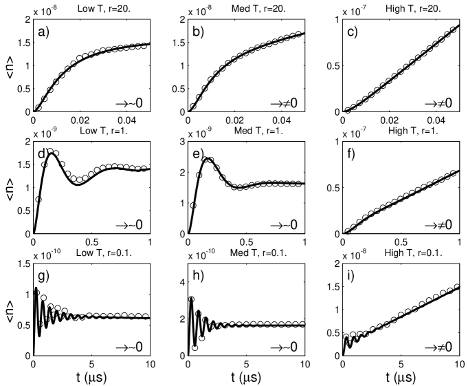
Figure 1: Dynamics of the heating function $\langle n(t)\rangle$ in the short time non-Markovian regime. For the high $T$, graphics (c),(f),(i), we have used $r_{0}=\omega_{0}/KT=0.1$; for the intermediate $T$, graphics (b),(e),(h) we have used $r_{0}=\omega_{0}/KT=1$; for low $T$, graphics (a),(d),(g), we have used $r_{0}=\omega_{0}/KT=100$. We indicate with solid line the analytic solution and with circles the simulations performed using the NMWF method. In the right-lower corner of all graphics we indicate whether the asymptotic long time value of the heating function is null (zero $T$ reservoir) or not.

For very low temperatures, the non-Markovian behavior of the heating function of the quantum Brownian particle may occur when $\langle n\rangle$ is of the order of $10^{-10}$, see Fig. 1. To reach such an accuracy, a MC simulation for the estimation of $\langle n\rangle$ would require more than $10^{10}$ realizations to be generated. This problem may be circumvented by an appropriate scaling of the time dependent coefficients $\Delta\left(t\right)\pm\gamma\left(t\right)$ of the master equation. The method is based upon the following considerations. Let us look at the properties of the Hilbert space path integral solution of the stochastic process corresponding to the unravelling of Eq. (20). The Hilbert space path integral representation is essentially the expansion of the propagator of the stochastic process $T\left[\theta,t|\theta_{0},t_{0}\right]$ in the number of quantum jumps petruccionebook :

$$T\left[\theta,t|\theta_{0},t_{0}\right]=\sum_{N=0}^{\infty}T^{(N)}\left[\theta,t|\theta_{0},t_{0}\right],$$ (40)

where $N$ denotes the number of jumps, and $T^{(N)}$ are the $N$ jump contributions to the propagator. As long as in the time evolution period of interest there is maximally one jump per realization, it can be shown that, in the weak coupling limit and for the initial conditions used here, the relevant contribution to the propagator is given by the first two terms $T^{(0)}$, $T^{(1)}$. In this case the expectation value of an arbitrary operator $O$ is given by

$$\langle O\rangle\left(t\right) = \int D\theta D\theta^{*}\langle\phi(t)|O|\psi(t)\rangle$$ (41)

$$\left\{T^{(0)}\left[\theta,t|\theta_{0},t_{0}\right]+T^{(1)}\left[\theta,t|\theta_{0},t_{0}\right]\right\}.$$

The contribution from $T^{(0)}$ gives the initial expectation value $\langle O\rangle\left(0\right)$ plus a term which is directly proportional to the decay coefficients $\Delta\pm\gamma$. Since $T^{(1)}$ is also directly proportional to the decay coefficients we get as a result that the change in the expectation value is also proportional to the decay coefficients

$$\langle O\rangle\left(t\right)-\langle O\rangle\left(0\right)\propto\Delta\pm\gamma.$$ (42)

Thus, to ease the numerics and still to obtain the correct result, it is possible to speed up the decay by multiplying the coefficients $\Delta\pm\gamma$ with some suitable factor $\beta$, and to do the corresponding scaling down by dividing the calculated ensemble average by the same factor at the end of the simulation. For the heating function the validity of the scaling can be seen directly from the analytic solution (see Eq.(45) of the following section). The scaling allows to reduce the ensemble size for the estimation of the heating function from the unpractical $10^{10}$ to the more practical $10^{4}-10^{5}$.

IV The Lindblad - non–Lindblad border

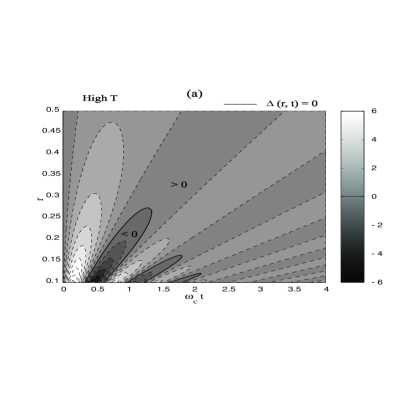
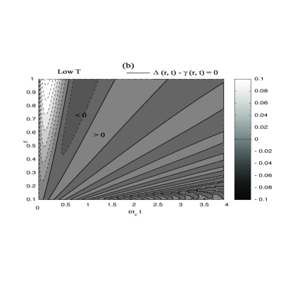
Figure 2: Contour plots of $\overline{\Delta(r,t)}=\Delta(r,t)/2\alpha^{2}KT$ for high $T$ (a), and of the coefficient $\overline{\Delta(r,t)-\gamma(r,t)}=[\Delta(r,t)-\gamma(r,t)]/\alpha^{2}$ for low $T$ (b). In (b) we have chosen $2\pi r_{c}=\hbar\omega_{c}/KT=10$. In both (a) and (b) the contour line corresponding to $\overline{\Delta(r,t)}=0$ (a) and $\overline{\Delta(r,t)-\gamma(r,t)}=0$ is indicated by a thick solid line.

This section contains the main results of the paper. Stimulated by the recent achievement in reservoir engineering techniques, we look at the dynamics of a quantum Brownian particle for different classes of reservoirs. We single out two reservoir parameters playing a key role in the dynamics of the open system, i.e. its temperature $T$ and the frequency cutoff $\omega_{c}$ of its spectral density. As we will see in this section, by varying these two parameters the time evolution of the system oscillator varies from Lindblad type to non-Lindblad type.

IV.1 Heating function

In order to illustrate the changes in the dynamics of the system we will focus, first of all, on the temporal behaviour of the heating function $\langle n(t)\rangle$. In the following section we will further investigate the non-Markovian time evolution by looking at the Mandel parameter, at the squeezing properties and at the Wigner function of the system.

Having in mind Eq. (16) and using Eq. (15), one gets the following expression for the heating function

$$\langle n(t)\rangle=e^{-\Gamma(t)}\langle n(0)\rangle+\frac{1}{2}\left(e^{-\Gamma(t)}-1\right)+\Delta_{\Gamma}(t),$$ (43)

with $\Delta_{\Gamma}(t)$ and $\Gamma(t)$ defined by Eqs. (18) and (19).

The asymptotic long time behavior of the heating function, for times $t$ much bigger than the reservoir correlation time $\tau_{R}=1/\omega_{c}$, is readily obtained by using the Markovian stationary values for $\Delta(t)$ and $\gamma(t)$, as given by Eqs. (55) - (56),

$$\langle n(t)\rangle=e^{-\Gamma t}\langle n(0)\rangle+n(\omega_{0})\left(1-e^{-\Gamma t}\right),$$ (44)

with $n(\omega_{0})=\left(e^{\hbar\omega_{0}/KT}-1\right)^{-1}$. This equation gives evidence for a second characteristic time of the dynamics, namely the thermalization time $\tau_{T}=1/\Gamma$, with $\Gamma=\alpha^{2}\omega_{0}r^{2}/(r^{2}+1)$. The thermalization time depends both on the coupling strength and on the ratio $r=\omega_{c}/\omega_{0}$ between the reservoir cutoff frequency and the system oscillator frequency. Usually, when studying QBM, one assumes that $r\gg 1$, corresponding to a natural Markovian reservoir with $\omega_{c}\rightarrow\infty$. In this case the thermalization time is simply inversely proportional to the coupling strength. For an “out of resonance”  engineered reservoir with $r\ll 1$, $\tau_{T}$ is notably increased and therefore the thermalization process is slowed down.

As we will see in the following, there exist other two characteristic timescales ruling the heating process: the period of the system oscillator $\tau_{S}=1/\omega_{0}$ and the thermal time $\tau_{\rm th}=1/\nu_{1}=1/2\pi kT$ defined as the inverse of the smallest positive Matsubara frequency. In Table 1 we summarize the definitions of the four time scales we have introduced up to now. In general the open system dynamics depends strongly on the relative value of these four characteristic time scales (see also haake2 ).

Let us consider now the dynamics of the heating function for times $t\ll\tau_{T}$. For simplicity we consider as initial condition the ground state of the system oscillator. The generalization to a generic initial state is however direct and similar conclusions hold. For times much smaller than the thermalization time, Eq. (43) can be approximated as follows:

$$\langle n(t)\rangle \simeq \int_{0}^{t}\left(\Delta(t_{1})-\gamma(t_{1})\right)dt_{1},$$ (45)

where Eq. (18) has been used. This equation shows that the initial dynamics of the heating function depends strongly on the sign of one of the time dependent coefficients of the secular master equation (12). The reason for the heating function to depend only on the coefficient $\Delta(t)-\gamma(t)$ and not on $\Delta(t)+\gamma(t)$ is simply related to the initial condition we have assumed. Indeed, when the initial state is the ground state of the oscillator, for times $t\ll\tau_{T}$, the probability of a jump up [absorbtion of a quantum of energy from the reservoir, see Eq.(38)] dominates over the probability of a jump down [emission of a quantum of energy into the reservoir, see Eq(39)]. This second process, which is the signature of the quantized nature of the reservoir, ensures the thermalization.

Table 1: Various time scales.

time scale name	symbol	explanation
reservoir correlation	$\tau_{R}=1/\omega_{c}$	$\omega_{c}=$ environment cutoff
thermalization	$\tau_{T}=1/\Gamma$	$\Gamma=\alpha^{2}\omega_{0}r^{2}/(r^{2}+1)$
system oscillator period	$\tau_{S}=1/\omega_{0}$	$\omega_{0}=$ oscillator frequency
thermal	$\tau_{\rm th}=1/\nu_{1}$	$\nu_{1}=$ Matsubara frequency
reservoir memory	$\tau_{corr}=\tau_{R}$	for high T
	$\tau_{corr}=\tau_{th}$	for medium T
	$\tau_{corr}=\tau_{S}$	for low T

Equation (45) shows us that the coefficient $\Delta(t)-\gamma(t)$ is the time derivative of the heating function. Therefore, if $\Delta(t)>\gamma(t)$ for all times $t\ll\tau_{T}$, the heating function grows monotonically, whereas if there exist intervals of time in correspondence of which $\Delta(t)<\gamma(t)$, the heating function decreases and eventually oscillates. We remind that, for the case considered here, whenever $\Delta(t)-\gamma(t)>0$ at all times, the master equation (12) is of Lindblad type, whilst if for some time intervals $\Delta(t)-\gamma(t)<0$ it is a non-Lindblad type master equation.

IV.2 Lindblad and non Lindblad regions

To better understand such a behavior we study in more details the dynamics for three different regimes of the ratio $r$ between the reservoir cutoff frequency and the system oscillator frequency: $r\gg 1$, $r=1$ and $r\ll 1$. The first case corresponds to the assumption commonly done when dealing with a natural reservoir while the last case corresponds to an engineered “out of resonance”  reservoir.

By using Eqs. (13) and (52), a straightforward but lengthy calculation shows that, for $r\gg 1$, $\Delta(t)>\gamma(t)>0$. In this case the master equation (12) is always of Lindblad type and the heating function is a monotonically growing function. The three upper graphics of Fig. 1 show the time evolution of the heating function for $r=20$ in the case of low (a), intermediate (b) and high (c) temperatures.

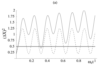
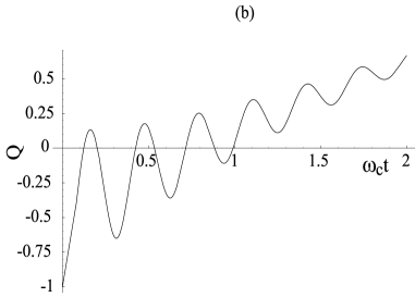
Figure 3: (a) Time evolution of the position variance for an initial squeezed state having squeezing parameter $s=0.4$. The reservoir parameters are $\alpha=10^{-2}$, $r=0.05$, and $r_{c}=\omega_{c}/2\pi KT=0.2\cdot 10^{-6}$. The dotted line shows the variance of the free harmonic oscillator in absence of coupling to the environment. The system exhibits squeezing whenever $\left(\Delta X\right)^{2}(t)<0.5$.
(b) Time evolution of the Mandel parameter for an initial Fock state $|n=3\rangle$. The reservoir parameters are the same as in (a)

.

In the case of an engineered “out of resonance”  reservoir, that is when $r\ll 1$, the sign of the diffusion coefficient is positive in the low temperature regime whilst for intermediate and high temperatures it assumes negative values for some time intervals. However, for intermediate and low temperatures, there exist intervals of time in correspondence of which $\Delta(t)-\gamma(t)<0$. Whenever $\Delta(t)-\gamma(t)$ is negative, the heating function decreases, so the overall heating process is characterized by oscillations as shown in Fig. 1 (g)-(h)-(i), where the dynamics of $\langle n(t)\rangle$ for low, intermediate and high $T$, respectively, and $r=0.1$ is plotted for $0<\omega_{c}t<10$. The decrease in the population of the ground state of the system oscillator, after an initial increase due to the interaction with the reservoir, is due to the emission and subsequent re-absorbtion of the same quantum of energy. Such an event is possible since the reservoir correlation time $\tau_{R}=1/\omega_{c}$ is now much longer than the period of oscillation $\tau_{s}=1/\omega_{0}$. We underline that, although the master equation in this case is not of Lindblad type, it conserves the positivity of the reduced density matrix. This of course does not contradict the Lindblad theorem since the semigroup property is clearly violated for the reduced system dynamics petruccionebook .

Finally, for $r=1$, one can show numerically that $\Delta(t)>0$ at all times whatever is the reservoir temperature $T$. Nonetheless, for intermediate and low temperatures the time dependent coefficient $\Delta(t)-\gamma(t)$ assumes negative values for some intervals of times. Such a situation leads again to an oscillatory behavior of the heating function as shown of Fig. 1(d) and Fig. 1 (e).

It is worth stressing that the non-Markovian features of the heating function discussed here do not depend on the secular approximation. Indeed, as we have mentioned in Sec. II, Eq. (43) coincides with the expression derived from the exact solution. Stated in another way, the appearance of virtual exchanges of energy between system and reservoir, characterizing the non-Lindblad region, is a general feature of the non-Markovian dynamics of the system and it is not connected with the secular approximation.

IV.3 The key parameters $r$ and $T$

The border between the Lindblad and non-Lindblad regions depends on two relevant reservoir parameters: its temperature $T$ and the ratio $r$ between its cutoff frequency and the system oscillator frequency. For high reservoir temperatures the quantity effectively ruling the dynamics is the diffusion coefficient $\Delta(t)$, since $\Delta(t)\gg\gamma(t)$. In other words, for short times and high $T$, diffusion is always dominant with respect to dissipation. Oscillatory dynamics of the heating function appears for $r\ll 1$ since $\Delta(t)$ oscillates assuming negative values. Figure 2 (a) shows a contour plot of $\Delta(r,t)$ for high $T$. The curve defined by the equation $\Delta(r,t)=0$ for high $T$, with $\Delta(r,t)$ given by Eq. (58), defines the Lindblad non-Lindblad border. From Fig. 2 (a) one can see that the largest value of $r$ in correspondence of which the system exhibits non-Lindblad oscillatory heating is $r\simeq 0.27$.

For decreasing temperatures the amplitude of $\Delta(t)$ becomes smaller and smaller. Thus, also in the presence of an oscillatory behavior of $\Delta(t)$, that is when $r\ll 1$, for low temperatures the diffusion coefficient remains always positive. In this case, however, dissipation is not negligible with respect to diffusion anymore and their combined action is such that, for intermediate and low temperatures, the non–Lindblad dynamics appears already for $r>1$ [see Fig.2 (b)]. Stated in another way, decreasing the temperature the oscillatory behavior of the heating function appears for higher values of the ratio $r$, which means that the non-Lindblad region becomes larger. Fig. 2 shows clearly that this region, corresponding to negative values of $\Delta(t)-\gamma(t)$ ($\Delta(t)$ for high $T$), is notably wider for low $T$ (b) than for high $T$ (a).

While in this section we have investigated the border between the Lindblad and non-Lindblad type regions, in the following section we will concentrate on the non-Lindblad type dynamics for two reasons. The first reason is that, in general, due to difficulties in dealing with non-Lindblad type master equations, only few studies have been carried out in this regime. Secondly, we have shown elsewhere that typical non-Lindblad dynamical features may be experimentally revealed in the trapped ion context with currently available technology Maniscalco04 .

V Non-Markovian dynamics of non-Lindblad type

In this section we focus on the dynamics of a quantum Brownian particle in the case of interaction with an engineered out of resonance reservoir, i.e. for $r\ll 1$. By using the techniques for reservoir engineering typical of trapped ion systems, such region of the parameter space is already in the grasp of the experimentalists. Indeed, by slightly modifying the experimental conditions used in Ref. engineerNIST , the oscillatory non-Markovian dynamics of the heating function can be measured Maniscalco04 .

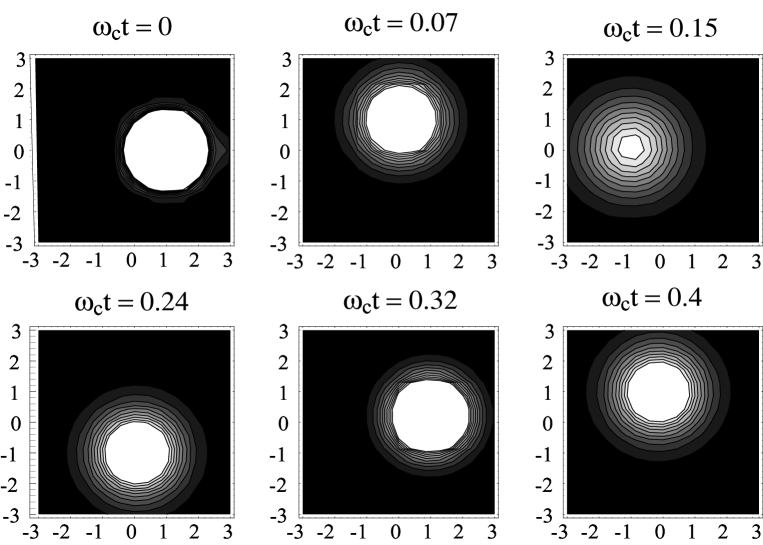
Figure 4: Contour plots of the Wigner function at different time instants. At $\tau=0$ the initial state is the coherent state correspondent to $Re[\alpha_{0}]=1$, $Im[\alpha_{0}]=0$. The reservoir parameters are $\alpha=10^{-2}$, $r=0.05$, and $r_{c}=\omega_{c}/2\pi KT=10^{-7}$.

In order to characterize completely the dynamics of the quantum Brownian particle in the non-Lindblad region we look at the dynamics of the squeezing, of the Mandel parameter and of the Wigner function for some exemplary initial states. We begin with the analysis of the squeezing in position. By using Eq. (15), it is possible to derive the following expression for the variance of the dimensionless position operator $X$:

$$\left(\Delta X\right)^{2}_{t} = e^{-\Gamma(t)}\left[\left(\Delta X\right)^{2}_{0}\cos^{2}(\omega_{0}t)+\left(\Delta P\right)^{2}_{0}\sin^{2}(\omega_{0}t)\right.$$ (46)

$$+ \left.C_{0}\sin(2\omega_{0}t)\right]+\Delta_{\Gamma}(t)$$

$$\equiv e^{-\Gamma(t)}(\Delta X)_{\rm f}(t)+\Delta_{\Gamma}(t),$$

where $\left(\Delta X\right)^{2}_{0}$ and $\left(\Delta P\right)^{2}_{0}$ are the initial variances of position and momentum operators, respectively, and $C_{0}=\frac{1}{2}(\langle X_{0}P_{0}+P_{0}X_{0}\rangle-\langle X_{0}\rangle\langle P_{0}\rangle)$ is the initial position-momentum correlation function. In the last line of Eq. (46) we have defined the function $(\Delta X)_{\rm f}(t)$ describing the time evolution of the variance of a quantum harmonic oscillator in absence of interaction with the environment. In the high temperature limit, it is not difficult to prove that the interaction with the environment generally causes an increase in the variance of the position operator with respect to its free dynamics. Indeed, for times much smaller than the thermalization time $t\ll\tau_{T}$, Eq. (46) may be approximated as follows

$$\!\!\left(\Delta X\right)^{2}_{t}\!\! \simeq \!\!(\Delta X)_{\rm f}(t)\!\!+\!\!\!\int_{0}^{t}\!\!\!\Delta(t_{1})-2(\Delta X)_{\rm f}(t_{1})\gamma(t_{1}),$$ (47)

where Eqs. (18)-(19) have been used. Having in mind that for high temperatures the condition $\Delta(t)\gg\gamma(t)$ holds, one realizes that, provided that $(\Delta X)_{free}(t)$ is not too big (corresponding to either a very high initial squeezing in position/momentum or a very high initial position-momentum correlation or a mixture of these cases), the integral appearing in Eq. (47) gives always a positive contribution. In the short time non-Markovian regime, for low reservoir temperatures, situations in which the system-environment correlations lead to a decrease in the squeezing in position, compared to its free time evolution, may in principle occur. Such a situation would be of interest since it could be exploited to generate squeezing through the interaction with an artificial low temperature reservoir. We plan to investigate further this point in the future.

In Fig. 3 (a) we plot the short time behavior of $\left(\Delta X\right)^{2}(t)$ for an initial squeezed state with squeezing factor $s=0.4$, that is with $\left(\Delta X\right)^{2}_{0}=s/2=0.2$ and $\left(\Delta P\right)^{2}_{0}=1/(2s)=0.8$. We remind that $X$ and $P$ are dimensionless, therefore squeezing in position corresponds to $\left(\Delta X\right)^{2}<0.5$. In the figure we compare the time evolution of the position variance for the damped harmonic oscillator with the case of the isolated harmonic oscillator. From the figure one sees clearly the effect of the virtual processes which tend to decrease the position variance and to bring it back to its initial value. The overall effect of the environment tends however to wash out the initial squeezing.

Let us now consider the time evolution of the Mandel parameter mandel

$$Q(t)=\frac{\langle n^{2}(t)\rangle-\langle n(t)\rangle^{2}}{\langle n(t)\rangle}-1.$$ (48)

This quantity gives an indication of the statistics of the quantized mode described by the system oscillator. For a Fock state $Q$ takes its lowest value $Q=-1$ while for a coherent state $Q$ is equal to $0$ . Therefore, values of $Q<0$ indicate subPoissonian statistics, while $Q=0$ characterizes Poissonian statistics and $Q>0$ superPoissonian statistics. Using Eq. (15) we have derived the time evolution of the Mandel parameter as follows

$$Q(t)\!=\!\frac{\langle n(t)\rangle^{2}\!\!+e^{-2\Gamma(t)}\!\langle n(0)\rangle\!\left[Q(0)-\!\langle n(0)\rangle\right]}{\langle n(t)\rangle}.$$ (49)

In Fig. 3 (b) we show the time evolution of the Mandel parameter for an initial Fock state $|n=3\rangle$. Due to the interaction with the artificial reservoir the initial temporal evolution is characterized by oscillations between subPossonian and Poissonian statistics of the quantized mode. This behaviour may be traced back to the virtual photon exchanges between the system and the reservoir and therefore is typical of the non-Markovian non-Lindblad-type region. Looking at Eq. (49), and remembering that $\Gamma(t)>0$ , and that $\langle n(t)\rangle\geq\langle n(0)\rangle$, it is easy to convince oneselves that, if the initial state is Poissonian or superPoissonian, i.e. $Q\geq 0$, the Mandel parameter will remain positive at all times. In other words, the interaction with the environment never creates subPoissonian statistics from an initial Poissonian or superPoissonian statistics. This conclusion is valid for generic temperatures $T$, provided that the weak coupling assumption is satisfied.

We now look at the the system dynamics in the non-Lindblad regime, considering the time evolution of the Wigner function of an initial coherent state $|\alpha_{0}\rangle$. Having in mind Eq. (16) and recalling that the Wigner function is simply the Fourier transform of the quantum characteristic function,

$$W(\alpha)=\frac{1}{\pi^{2}}\int_{-\infty}^{\infty}d^{2}\xi\chi(\xi)e^{\alpha\xi^{*}-\alpha^{*}\xi},$$ (50)

one gets

$$W_{t}(\alpha)=\frac{1}{\pi\left[\Delta_{\Gamma}(t)+1/2\right]}\exp\left[\frac{\left|\alpha_{0}e^{-\Gamma(t)/2}e^{-i\omega_{0}t}-\alpha\right|^{2}}{\Delta_{\Gamma}(t)+1/2}\right].$$ (51)

From this equation and from Fig. (4) one sees clearly that the system-reservoir interaction spreads the initial Wigner function. Breathing of the Wigner function, that is the oscillation in its spread, appears in correspondence of the virtual processes. This is a new dynamical feature which is absent both in the Markovian dynamics of the damped harmonic oscillator and in the Lindblad-type non-Markovian dynamics. Indeed, in both the previous regimes, the spread in the Wigner function simply increases, linearly in time in the Markovian case, and quadratically in time in the non-Markovian Lindblad-type case. We note that different breathing scenarios for the second moments in different regimes have been discussed in henkel .

In summary, the exchanges of energy between system and reservoir characterizing the non-Lindblad type region strongly influence the dynamics of the system. In general, if the initial state of the oscillator possesses nonclassical properties (as squeezing or subPoissonian statistics), the interaction with the environment tends to wash out such properties in a time scale which is dependent, as one would guess, on the reservoir parameters (spectral density and temperature). In this section we have considered a high $T$ engineered ‘out of resonance’(i.e. with $r\ll 1$) reservoir. In this case the loss of nonclassical properties appears in a time scale which is smaller or equal to the reservoir correlation time $\tau_{R}=1/\omega_{c}$. Moreover, the effect of the virtual processes, which is also important in this time scale, may cause oscillations between classical and nonclassical states, as in the case shown in Fig. 3 (b). It is worth noting that, in the situation here considered, the loss of nonclassical properties, as well as the oscillations due to virtual processes, happen in a time scale which is in general much shorter than the decoherence time $\tau_{\rm dec}=\lambda_{T}^{2}/(d^{2}\alpha^{2})$, with $d$ separation between the two components of a quantum superposition and $\lambda_{T}=\hbar/\sqrt{2mkT}$ de Broglie wavelenght zurekrev . This is clearly related to the high temperature condition of interest here, which implies $\tau_{R}\gg 1/KT$.

In order to give a more quantitative estimate one should, however look at some specific physical system, in order to fix also the other quantities appearing in the definition of the two time scales. To this aim we consider the recent experiment with trapped ions in which the decoherence of different superpositions of the vibrational motion of the center of mass of the ion was observed engineerNIST . For this system, this experiment has shown that decoherence of a superpositon of two Fock states happens on a time scale of the order of $30\mu$s. Very recently we have proposed an experiment Maniscalco04 to observe non-Markovian features of the heating function in the same system and with the same set up used in engineerNIST . According to our calculations, by slightly modifying the experimental parameters used, one could observe oscillations in the heating function in a time scale of the order of $3\mu$s, that is one order of magnitude less than the decoherence time measured in that system for a superposition of Fock states.

In conclusion, the investigation carried out in this section sheds light on the short time dynamics of the damped harmonic oscillator, focussing in particular on the high $T$ regime. Further analysis of the squeezing, of the Mandel parameter and of the Wigner function may bring new insight in the time scales governing the loss of nonclassical properties and in their relationship with the decoherence and dissipation time scales. We plan to explore further this aspect, with particular attention to the low temperature case.

VI Conclusions

In this paper we have studied the short time non-Markovian dynamics of a quantum Brownian particle moving in a harmonic potential. The dynamics of this paradigmatic open quantum system is described by a non-Markovian master equation which is local in time. This master equation cannot be recast in the Lindblad form. Nevertheless, under certain conditions, the master equation for quantum Brownian motion is of Lindblad type, i.e. it has the same operatorial form of the Lindblad master equation but with time dependent (instead of constant) positive coefficients.

In the weak coupling limit, the relevant time dependent coefficients can be cast in a closed form. In this case by using the exact analytic solution in terms of the quantum characteristic function, we have identified the parameters governing the passage from Lindblad type to non-Lindblad type master equation. These parameters are the reservoir temperature $T$ and the ratio $r$ between the frequency $\omega_{0}$ of the system oscillator and the reservoir cutoff frequency $\omega_{c}$. It is worth stressing that the weak coupling limit we consider in the paper is of interest also in the light of the engineering of reservoir experiments. In fact, in order to observe experimentally the key features of the system-reservoir interaction, e.g. the role played by the entanglement between system and reservoir in the decoherence process, the coupling between system and reservoir does not have to be too strong. The stronger is the coupling the faster is the establishment of quantum correlations between the system and the environment, and the more difficult is the experimental observability of their dynamics. For this reason the techniques of reservoir engineering, allowing to control both the coupling constant and other reservoir parameters as its spectral density, look very promising for investigating fundamental issues as the quantum-classical border.

Our analysis of the short time non-Markovian region shows that the Lindblad type dynamics is characterized by a monotone increase of the heating function, and therefore of the energy, of the open system. In the non-Lindblad type region, on the contrary, oscillations in the mean energy of the system clearly indicate the occurrence of virtual exchanges of energy between the system and the reservoir. Lowering the reservoir temperature increases the probability that virtual processes take place.

It is worth noting that whenever the master equation for the system is of Lindblad type, it is possible to apply the standard MC simulation schemes and there exists a direct correspondence between the MC simulation method and a continuous measurement scheme Dalibard92a ; Molmer93a ; Molmer96a . For more general non-Markovian Monte Carlo methods, e.g. the NMWF we have used in this paper, an analogous correspondence would be of interest. There are indications that the Lindblad non-Lindblad border might be identified with the border between existence and non-existence of a measurement scheme interpretation for non Markovian stochastic methods. For this reason, the study of the dependence of this border from parameters as the reservoir temperature and the ratio $r$ might give some insight and useful hints to the research on this contemporary topic.

Finally, last part of our paper deals with an analytic description of the short time dynamics of the quantum Brownian particle when virtual processes dominate. We have investigated in detail the temporal evolution by looking at the squeezing properties, at the Mandel $Q$ parameter and at the Wigner function. We have found that, if the system initially possesses nonclassical properties as squeezing in one of the quadratures or non-Poissonian statistics, these properties tend to be washed out due to the interaction with the reservoir. However oscillations between squeezing and non-squeezing as well as between sub-Poissonian and Poissonian statistics appears in connection with the virtual exchanges of energy. A further sign of the virtual processes is the breathing in the width of the Wigner function.

Summarizing, the main result of this paper is the detailed analysis of the non-Markovian features characterizing the dynamics of a quantum Brownian particle, with special attention to the appearance of virtual processes for certain ranges of reservoir temperature and cutoff frequency. Due to the generality of the model here studied we think that our results can both contribute to fundamental research on open quantum systems and, when applied to specific physical contexts, shed light on their dynamics.

VII Acknowledgements

The authors gratefully acknowledge Heinz-Peter Breuer for helpful comments and stimulating discussions. J.P. acknowledges financial support from the Academy of Finland (projects 50314 and 204777), and from the Magnus Ehrnrooth Foundation; and the Finnish IT center for Science (CSC) for computer resources. J.P. and F.P. thank the University of Palermo for the hospitality. J.P. and S.M. acknowledge the EU network COCOMO (contract HPRN-CT-1999-00129) for financial support. S.M. acknowledges the Angelo Della Riccia Foundation for financial support and the Helsinki Institute of Physics for the hospitality.

Appendix A Diffusion coefficient

In order to derive a closed analytic expression for $\Delta(t)$ valid for all temperatures and for all values of the ratio $r$ we integrate Eq. (10) and use the series expansion of the hypergeometric function:

$$\Delta(t) = \alpha^{2}\omega_{0}\frac{r^{2}}{1+r^{2}}\Big{\{}\coth(\pi r_{0})-\cot(\pi r_{c})e^{-\omega_{c}t}\left(r\cos(\omega_{0}t)-\sin(\omega_{0}t)\right)$$ (52)

$$+ \frac{1}{\pi r_{0}}\cos(\omega_{0}t)\left[\bar{F}(-r_{c},t)+\bar{F}(r_{c},t)-\bar{F}(ir_{0},t)-\bar{F}(-ir_{0},t)\right]$$

$$- \frac{1}{\pi}\sin(\omega_{0}t)\Big{[}\frac{e^{-\nu_{1}t}}{2r_{0}(1+r_{0}^{2})}\left((r_{0}-i)\bar{G}(-r_{0},t)+(r_{0}+i)\bar{G}(r_{0},t)\right)$$

$$+ \frac{1}{2r_{c}}\left(\bar{F}(-r_{c},t)-\bar{F}(r_{c},t)\right)\Big{]}\Big{\}}.$$

In this equation we have used the notations $r_{0}=\omega_{0}/2\pi kT$, $r_{c}=\omega_{c}/2\pi kT$,

$$\bar{F}(x,t) \equiv {}_{2}F_{1}\left(x,1,1+x,e^{-\nu_{1}t}\right)$$ (53)

$$\bar{G}(x,t) \equiv {}_{2}F_{1}\left(2,1+x,2+x,e^{-\nu_{1}t}\right),$$ (54)

where ${}_{2}F_{1}\left(a,b,c,z\right)$ is the hypergeometric function tavole .

Appendix B Markovian and High Temperature limits

In the asymptotic long time limit, the time dependent coefficients $\gamma(t)$ and $\Delta(t)$ tend to their stationary value given by

$$\Delta_{M} \equiv \Delta(t\rightarrow\infty)=\alpha^{2}\omega_{0}\frac{r^{2}}{1+r^{2}}\coth(\omega_{0}/2kT)$$ (55)

$$\gamma_{M} \equiv \gamma(t\rightarrow\infty)=\alpha^{2}\omega_{0}\frac{r^{2}}{1+r^{2}},$$ (56)

and the master equation (12) becomes the well known Markovian master equation for a damped quantum harmonic oscillator

$$\frac{d\rho_{S}}{dt}= - \Gamma[n(\omega_{0})+1]\left[a^{{\dagger}}a\rho_{S}-2a\rho_{S}a^{{\dagger}}+\rho_{S}a^{{\dagger}}a\right]$$ (57)

$$- \Gamma n(\omega_{0})\left[aa^{{\dagger}}\rho_{S}-2a^{{\dagger}}\rho_{S}a+\rho_{S}aa^{{\dagger}}\right],$$

with $\Gamma=\alpha^{2}\omega_{0}r^{2}/(1+r^{2})$ and $n(\omega_{0})=\left(e^{\omega_{0}/kT}-1\right)^{-1}$.

As far as the high temperature limit is concerned, having in mind the definitions of $r_{0}$ and $r_{c}$, one sees immediately that such an approximation amounts at taking $r_{0},r_{c}\ll 1$, that is $x\ll 1$. Under this condition one has tavole :

$$\bar{F}(x,t) = {}_{2}F_{1}\left(x,1,1+x,e^{-\nu_{1}t}\right)$$

$$\simeq {}_{2}F_{1}\left(x,1,1,e^{-\nu_{1}t}\right)=\left(1-e^{-\nu_{1}t}\right)^{-a},$$

$$\bar{G}(x,t) = {}_{2}F_{1}\left(2,1+x,2+x,e^{-\nu_{1}t}\right)$$

$$\simeq {}_{2}F_{1}\left(2,1,2,e^{-\nu_{1}t}\right)=\left(1-e^{-\nu_{1}t}\right)^{-1}.$$

Inserting these expressions in Eq. (52) and using the approximations

$$\cot(\pi r_{c}) \simeq \frac{1}{\pi r_{c}}=\frac{2kT}{\omega_{c}},$$

$$\coth(\pi r_{0}) \simeq 1+\frac{1}{\pi r_{0}}\simeq\frac{2kT}{\omega_{0}}$$

one gets the Caldeira-Leggett high temperature expression for $\Delta(t)$ Caldeira

$$\Delta(t)^{HT} = 2\alpha^{2}kT\frac{r^{2}}{1+r^{2}}\left\{1-e^{-\omega_{c}t}\left[\cos(\omega_{0}t)\right.\right.$$ (58)

$$- (1/r)\left.\left.\sin(\omega_{0}t)\right]\right\}.$$

The other time dependent coefficient, $\gamma(t)$, does not depend on temperature as one can easily see by Eq. (4). We stress that, comparing Eq. (58) with Eq. (13), one notices immediately that in the high temperature regime, $\Delta(t)\gg\gamma(t)$.

References

- (1) H.-P. Breuer and F. Petruccione, The Theory of Open Quantum systems (Oxford University Press, 2002).
- (2) G. Lindblad, Commun. Math. Phys. 48, 119 (1976).
- (3) V. Gorini, A. Kossakowski, and E.C.G. Sudarshan, J. Math. Phys. 17, 821 (1976).
- (4) K. Mølmer and Y. Castin, Quantum Semiclass. Opt. 8, 49 (1996).
- (5) T. Quang, M. Woldeyohannes, S. John, and G. S. Agarwal, Phys. Rev. Lett. 79, 5238 (1997); S. John and T. Quang, Phys. Rev. Lett. 78, 1888 (1997).
- (6) J. J. Hope, G. M. Moy, M. J. Collett, and C. M. Savage, Phys. Rev. A 61, 023603 (2000).
- (7) E. Joos, H.-D. Zeh, C. Kiefer, D. Giulini, J. Kupsch, and I.-O. Stamatescu, Decoherence and the Appearence of a Classical World in Quantum Theory, 2nd ed. (Springer-Verlag, Berlin, 2003).
- (8) M. A. Nielsen and I. L. Chuang, Quantum Computation and Quantum Information (Cambridge University Press, Cambridge, England, 2000).
- (9) C. J. Myatt et al., Nature 403, 269 (2000); Q.A. Turchette et al., Phys. Rev. A 62, 053807 (2000).
- (10) J.F. Poyatos, J.I. Cirac, and P. Zoller, Phys. Rev. Lett. 77, 4728 (1996).
- (11) M.B. Plenio and S.F. Huelga, Phys. Rev. Lett. 88, 197901 (2002).
- (12) J. Eisert and M. B. Plenio, Phys. Rev. Lett. 89, 137902 (2002).
- (13) P.J. Dodd and J. J. Halliwell, Phys. Rev. A 69, 052105 (2004).
- (14) F. Haake and R. Reibold, Phys. Rev. A 32, 2462 (1985).
- (15) H.-P. Breuer, B. Kappler, and F. Petruccione, Ann. Phys. 291, 36 (2001).
- (16) R.P. Feynman and F.L. Vernon, Ann. Phys. 24, 118 (1963).
- (17) A.O. Caldeira and A.J. Leggett, Phys. A 121, 587 (1983).
- (18) B.L. Hu, J.P. Paz and Y. Zhang, Phys. Rev. D 45, 2843 (1992).
- (19) G.W. Ford and R.F. O’Connell, Phys. Rev. D 64, 105020 (2001).
- (20) H. Grabert, P. Schramm, and G.-L. Ingold, Phys. Rep. 168, 115 (1988).
- (21) F. Intravaia, S. Maniscalco, and A. Messina, Phys. Rev. A 67, 042108 (2003).
- (22) F. Intravaia, S. Maniscalco, J. Piilo, and A. Messina, Phys. Lett. A 308, 6 (2003).
- (23) F. Intravaia, S. Maniscalco, and A. Messina, Eur. Phys. J. B 32, 97 (2003).
- (24) S. Maniscalco, F. Intravia, J. Piilo, and A. Messina, J. Opt. B: Quantum Semiclassical Opt. 6, S98 (2004).
- (25) H. P. Breuer, B. Kappler, and F. Petruccione, Phys. Rev. A 59, 1633 (1999).
- (26) J. Dalibard, Y. Castin, and K. Mølmer, Phys. Rev. Lett. 68, 580 (1992).
- (27) K. Mølmer, Y. Castin, and J. Dalibard, J. Opt. Soc. Am. B 10, 524 (1993).
- (28) M. B. Plenio and P. L. Knight, Rev. Mod. Phys. 70, 101 (1998) and references therein.
- (29) H.-P. Breuer, Phys. Rev. A 69, 022115 (2004).
- (30) S. Chaturvedi and J. Shibata, Z. Phys. B 35, 297 (1979); N.H.F. Sgibata and Y. Takahashi, J. Stat. Phys. 17, 171 (1977).
- (31) A. Royer, Phys. Rev. A 6, 1741 (1972); A. Royer, Phys. Lett. A 315, 335 (2003).
- (32) R. Karrlein and H. Grabert, Phys. Rev. E 55, 153 (1997).
- (33) C. Cohen-Tannoudj, J. Dupont-Roc, and G. Grynberg, Atom-Photon Interactions (John Wiley and Sons, New York, 1992).
- (34) J. Piilo, K.-A. Suominen, and K. Berg-Sørensen, Phys. Rev. A 65, 033411 (2002).
- (35) J. Piilo, J. Opt. Soc. Am. B 20, 1135 (2003), Feature Issue on Laser Cooling of Matter.
- (36) W.T. Strunz and F. Haake, Phys. Rev. A 67, 022102 (2003).
- (37) S. Maniscalco, J. Piilo, F. Intravaia, F. Petruccione and A. Messina, Phys. Rev. A 69, 052101 (2004).
- (38) L. Mandel and E. Wolf, Optical Coherence and Quantum Optics, (Cambridge University Press, 1995).
- (39) C. Henkel, M. Nest, P. Domokos, and R. Folman, Model for the observation of the spatial decoherence of a massive object, quant-ph/0310160.
- (40) W. H. Zurek, Rev. Mod. Phys 75, 715 (2003).
- (41) I.S. Gradshtein and I.M. Ryzhik, Tables of Integrals, Series and Products (Academic Press Inc., 1994).