Quantum walks and their algorithmic applications

Abstract

Quantum walks are quantum counterparts of Markov chains. In this article, we give a brief overview of quantum walks, with emphasis on their algorithmic applications.

1 Introduction

Markov chains have an important role in randomized algorithms (for example, algorithms for approximating permanent and other hard problems and volume estimation [1]). Recently, quantum counterparts of Markov chains have been defined [2, 3, 4, 5], with the hope that they could have similar applications in design of new quantum algorithms. It was immediately noticed that quantum walks behave quite differently from their classical counterparts. Recently, several algorithms using quantum walks have been invented.

In this paper, we survey results on algorithmic applications of quantum walks. Sections 2 and 3 give the background on quantum walks. In particular, section 2 explains basics of quantum walks, using quantum walk on the line as an example. Then, in section 3 we show how to define a quantum walk on an arbitrary graph. After that, in sections 4 and 5, we describe the known algorithms that use quantum walks. Those algorithms can be classified into two groups: algorithms achieving exponentially faster hitting times [6, 7, 8, 9] and quantum walk search [10, 11, 12, 13]. We describe the first group in section 4 and the second group in section 5. At the conclusion, we present some open problems in section 6.

Besides the algorithmic aspects described in the current paper, there are many other interesting results about quantum walk. We refer the reader to an excellent survey by Kempe [14] for more information about quantum walks in general.

2 Quantum walk on the line

Quantum walk on a line is a simple example which shows many properties of quantum walks. It is also often useful as a tool in the analysis of quantum walks on more complicated graphs. (We will show two examples of that in sections 4 and 5.)

2.1 Discrete quantum walk

In a classical random walk on the line, we start in location 0. At each time step, we move left with probability 1/2 and right with probability 1/2.

The straightforward counterpart would be a quantum process with basis states $|n\rangle$, $n\in Z$. At each time step, it would perform a unitary transformation

$$|n\rangle\rightarrow a|n-1\rangle+b|n\rangle+c|n+1\rangle,$$ (1)

which means move left with some amplitude $a$, staying at the same place with amplitude $b$ and moving right with amplitude $c$. Moreover, we would like the process to behave in the same way in every location. That is, $a$, $b$ and $c$ should be independent of $n$ (just like the probabilities of moving left/right are independent of $n$ in the classical walk). Unfortunately, this definition does not work.

Theorem 1

[3] The transformation $U$ defined by equation (1) is unitary if and only if one of following three conditions is true:

1. $|a|=1$, $b=c=0$;

2. $|b|=1$, $a=c=0$;

3. $|c|=1$, $a=b=0$;

Thus, the only possible transformations are the trivial ones (ones that, at each step, either always move left or always stay in place or always move right). The same problem also appears when defining quantum walks on many other graphs.

It can be solved by introducing an additional “coin” state. We consider the state space consisting of states $|n,0\rangle$ and $|n,1\rangle$ for $n\in Z$. At each step, we do two operations:

1. A “coin flip transformation” $C$

   $$C|n,0\rangle=a|n,0\rangle+b|n,1\rangle,$$

   $$C|n,1\rangle=c|n,0\rangle+d|n,1\rangle.$$

2. Shift $S$:

   $$S|n,0\rangle=|n-1,0\rangle,\mbox{~{}~{}}S|n,1\rangle=|n+1,1\rangle.$$

A step of quantum walk is $SC$. The most common choice for $C$ is the Hadamard transformation

$$\left(\begin{array}[]{cc}a&b\\ c&d\end{array}\right)=\left(\begin{array}[]{cc}\frac{1}{\sqrt{2}}&\frac{1}{\sqrt{2}}\\ \frac{1}{\sqrt{2}}&-\frac{1}{\sqrt{2}}\end{array}\right).$$ (2)

Any other unitary transformation in 2-dimensions can be also used.

We can think of $C$ as a quantum counterpart of coin flip in which we decide in which direction to move. To see this analogy, consider the modification in which, between $C$ and $S$, we measure the state. If the state before $C$ is $|n,0\rangle$, then the state after $C$ is $\frac{1}{\sqrt{2}}|n,0\rangle+\frac{1}{\sqrt{2}}|n,1\rangle$ and measuring it yields $|n,0\rangle$ and $|n,1\rangle$ with probabilities 1/2 each. If the state before $C$ is $|n,1\rangle$, then the state after $C$ is $\frac{1}{\sqrt{2}}|n,0\rangle-\frac{1}{\sqrt{2}}|n,1\rangle$. Measuring this state also yields $|n,0\rangle$ and $|n,1\rangle$ with probabilities 1/2 each. Thus, $C$ is now equivalent to probabilistically picking one of $|n,0\rangle$ and $|n,1\rangle$ with probabilities 1/2 each.

However, in the quantum coin flip we do not measure the state. This leads to a clearly different results. Consider the first three steps of quantum walk, starting in state $|0,0\rangle$.

$$|0,0\rangle\rightarrow\frac{1}{\sqrt{2}}|0,0\rangle+\frac{1}{\sqrt{2}}|0,1\rangle\rightarrow\frac{1}{\sqrt{2}}|-1,0\rangle+\frac{1}{\sqrt{2}}|1,1\rangle\rightarrow$$

$$\frac{1}{2}|-1,0\rangle+\frac{1}{2}|-1,1\rangle+\frac{1}{2}|1,0\rangle-\frac{1}{2}|1,1\rangle\rightarrow$$

$$\frac{1}{2}|-2,0\rangle+\frac{1}{2}|0,1\rangle+\frac{1}{2}|0,0\rangle-\frac{1}{2}|2,1\rangle\rightarrow$$

$$\frac{1}{2\sqrt{2}}|-2,0\rangle+\frac{1}{2\sqrt{2}}|-2,1\rangle+\frac{1}{\sqrt{2}}|0,0\rangle-\frac{1}{2\sqrt{2}}|2,0\rangle+\frac{1}{2\sqrt{2}}|2,1\rangle\rightarrow$$

$$\frac{1}{2\sqrt{2}}|-3,0\rangle+\frac{1}{2\sqrt{2}}|-1,1\rangle+\frac{1}{\sqrt{2}}|-1,0\rangle-\frac{1}{2\sqrt{2}}|1,0\rangle+\frac{1}{2\sqrt{2}}|3,1\rangle.$$

The result of first two steps is quite similar to classical random walk. If, after the second step, we measured the state, we would find $n=-2$ and $n=2$ with probability 1/4 and $n=0$ with probability 1/2. This is exactly what we would have had in a classical random walk.

The third step is different. In the coin flip stage, the state $\frac{1}{2}|0,1\rangle+\frac{1}{2}|0,0\rangle$ gets mapped to $\frac{1}{\sqrt{2}}|0,0\rangle$. In the classical random walk, we would choose left and right direction with probabilities 1/2 each. In the quantum case, we end up going to the left with all the amplitude. This is the result of quantum interference.

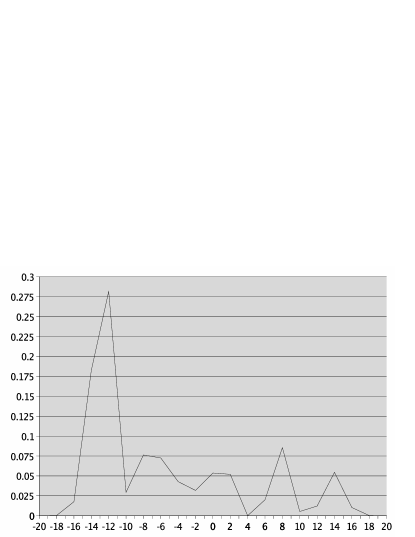
Figure 1: Probability distribution of quantum walk after 20 steps with coin flip (2).

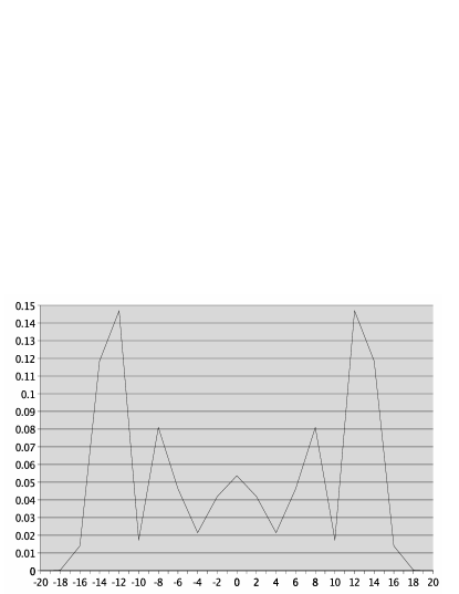
Figure 2: Probability distribution of quantum walk after 20 steps with coin flip (3).

The difference becomes more striking as large times are considered. If we start at location 0 and run classical random walk for $t$ steps, the probability distribution approaches normal distribution. In the quantum case, the corresponding experiment would be starting quantum walk in the state $|0,0\rangle$, running $t$ steps of quantum walk (which result in the transformation $(SC)^{t}$) and measuring the final state. This yields probability distribution of the form shown in figure 2 which is very different from the normal distribution.

First, the distribution is biased towards left. The drift to the left is a consequence of slightly non-symmetric coin flip transformation. (In equation (2), the amplitude of going from $|n,0\rangle$ to $|n,0\rangle$ is $a=\frac{1}{\sqrt{2}}$ but the amplitude of going from $|n,1\rangle$ to $|n,1\rangle$ is $d=-\frac{1}{\sqrt{2}}$.) It disappears if more symmetric coin

$$\left(\begin{array}[]{cc}\frac{1}{\sqrt{2}}&\frac{i}{\sqrt{2}}\\ \frac{i}{\sqrt{2}}&\frac{1}{\sqrt{2}}\end{array}\right)$$ (3)

is used. The probability distribution for this coin transformation is shown in figure 2. Two other quantum effects remain for almost any choice of coin transformation and starting state[5, 15].

1. The maximum probability is reached for $|n|\approx\pm\frac{t}{\sqrt{2}}$.

2. There are $\Omega(t)$ locations $n$ for which the probability of measuring $|n,0\rangle$ or $|n,1\rangle$ is $\Omega(\frac{1}{t})$. This means that the expected distance between the starting location $0$ and the location which we measure after $t$ steps is $\Omega(t)$.

Both of those sharply contrast with the classical random walk. In the classical random walk, the maximum probability is reached for $n\approx 0$. This has a simple intuitive explanation: the number of steps to the left is approximately equal to the number of steps to the right. Second, the probability of being more than $O(\sqrt{t})$ steps from the origin at time $t$ is negligible.

Can we exploit any of those properties to design fast quantum algorithms? The second property seems to be most promising. It means that quantum walk spreads quadratically faster than its classical counterpart.

The probability distribution generated by running quantum walk for $t$ steps and measuring it has been studied in more detail in refs. [5, 15, 16, 17, 18]. Other interesting quantum effects appear if we add boundary conditions to the line [5, 19, 20].

2.2 Continous walk

Farhi and Gutman [6] have defined continous time quantum walk. In continous time, introducing “coin” state is not necessary. Instead, one can define walk on the line on the set of states $|n\rangle$, $n\in Z$. To do that, we take Hamiltonian $H$ defined by $H|n\rangle=-|n-1\rangle+2|n\rangle-|n+1\rangle$. Running quantum walk for time $t$ is just applying the transformation $U^{iHt}$.

The results about discrete and continous walk are often similar but the relation between the two is unclear. In the classical world, continous walk can be obtained as a limit of the discrete walk. In quantum case, this does not seem to be true because discrete walk has a coin but continous walk does not.

3 Quantum walks on general graphs

How do we generalize the quantum walk on the line to more general graphs? Continous walk can be extended to a general graph quite easily [7]. We take Hamiltonian $H$ defined by $H_{ij}=-1$ if $i\neq j$ and vertices $i$ and $j$ are connected by an edge and $H_{ii}=d_{i}$ where $d_{i}$ is the degree of vertex $i$. Then, running quantum walk for time $t$ is just applying the transformation $e^{iHt}$.

For discrete quantum walk, defining it on an arbitrary graph is more difficult. The first papers [4] only defined it on graphs where every vertex has the same number of outgoing edges. However, there is a simple way to define a quantum walk on an arbitrary undirected graph.

Let $V$ be the set of vertices and $E$ be the set of edges. We use basis states $|v,e\rangle$ for all $v\in V$ and $e\in E$ such that the edge $e$ is incident to the vertex $v$. One step of quantum walk now consists of the following:

1. For each $v$, we perform a coin flip transformation $C_{v}$ on the states $|v,e\rangle$, $e$ adjacent to $v$.

2. We perform shift $S$ defined as follows. If edge $e$ has endpoints $v$ and $v^{\prime}$, then $S|v,e\rangle=|v^{\prime},e\rangle$ and $S|v^{\prime},e\rangle=|v,e\rangle$.

A very natural choice for $C_{v}$ is Grover’s diffusion (first used in Grover’s search algorithm[23]). If there are $m$ edges $e$ incident to vertex $v$, we apply the transformation described by matrix

$$D_{m}=\left(\begin{array}[]{cccc}-1+\frac{2}{m}&\frac{2}{m}&\ldots&\frac{2}{m}\\ \frac{2}{m}&-1+\frac{2}{m}&\ldots&\frac{2}{m}\\ \ldots&\ldots&\ldots&\ldots\\ \frac{2}{m}&\frac{2}{m}&\ldots&-1+\frac{2}{m}\end{array}\right)$$

to states $|v,e\rangle$. The logic behind this transformation is very simple. Typically, we would like to treat all edges adjacent to $v$ in the same way. Thus, the amplitude of staying in the same state $|v,e\rangle$ should be the same for all $e$. Similarly, for all $e$ and $e^{\prime}$, $e\neq e^{\prime}$, the amplitude of moving from $|v,e\rangle$ to $|v,e^{\prime}\rangle$ should be the same for all $e$ and $e^{\prime}$. The transformation $D_{m}$ satisfies these requirements. Moreover, the only unitary matrices with real entries satisfying this requirement are $D_{m}$, $-D_{m}$, $I$ (identity) and $-I$. Since $I$ leads to trivial results (if we go from $v^{\prime}$ to $v$ via edge $e$ in one step, we go back to $v^{\prime}$ via the same edge in the next step), $D_{m}$ is the natural choice.

A possible exception is if $v$ has exactly two edges adjacent to it. Then, $D_{m}$ is equal to the matrix.

$$\sigma_{x}=\left(\begin{array}[]{cc}0&1\\ 1&0\end{array}\right)$$

A possible alternative in this case is the matrix of equation (3) which is complex valued but treats both of adjacent vertices in the same way.

Next, we describe the known quantum algorithms using quantum walks. They can be broadly classified into two groups.

4 Exponentially faster hitting

The algorithms of this type include [6, 7, 8, 9]. In this group of algorithms, we have a known graph $G$. We start in one vertex $A$ and would like to reach a certain target vertex $B$. For example, in [7], we have the graph shown in figure 3 and would like to go from the left vertex $A$ to the right vertex $B$. At one step, we can choose one of edges adjacent to the current vertex and move to the other endpoint of this vertex. The difficulty is that edges and vertices are not labelled and we do not know which of possible moves takes us in the right direction.

One solution would be to do classical random walk, starting from $A$. Then, the number of steps till we first enter $B$ is typically polynomial in the number of vertices of $G$. For graphs with regular structure, quantum walks can do much better. For example[7], consider two full binary trees of depth $d$ with roots $A$ and $B$. Glue each leaf of the first tree with a leaf of the second tree. The resulting graph is shown in figure 3. It has $O(2^{d})$ vertices. If we start in $A$ and do a classical random walk, it will take $\Omega(2^{d})$ steps to reach $B$.

Childs et al. [7] showed that a continous quantum walk on $G$ can reach $B$ from $A$ in $O(d^{2})$ steps. They take basis states $|i\rangle$ with $i$ corresponding to vertices of $G$ and define a Hamiltonian $H$ by $H_{ij}=-1$ if $i,j$ are adjacent and $H_{ii}=d_{i}$ (as described in section 3). Then, $t$ steps of quantum walk is just the unitary transformation $E^{iHt}$.

Figure 3: “Glued trees” graph of Childs, Farhi and Gutman [7].

It might seem that analyzing quantum walk on $G$ is more difficult than analyzing the walk on line (because $G$ has a more complicated structure). However, there is a clever reduction to the walk on line [7]. Partition vertices into $2d+1$ sets $S_{-d}$, $S_{-d+1}$, $\ldots$, $S_{d}$. The set $S_{-d}$ contains just the vertex $A$. The set $S_{-d+i}$ contains vertices which are reached by walking $i$ edges to the right from $A$. In particular, $S_{0}$ contains all the vertices of degree 2 in the middle and $S_{d}$ contains just the vertex $B$. It is easy to see that $|S_{i}|=|S_{-i}|=2^{d-i}$. We define $|\psi_{i}\rangle=\frac{1}{\sqrt{|S_{i}|}}\sum_{v\in S_{i}}|v\rangle$. Let ${\cal H}$ be the subspace spanned by states $|\psi_{i}\rangle$, $i\in\{-d,-d+1,\ldots,d\}$. Then, it can be shown[7] that Hamiltonian $H$ maps ${\cal H}$ to itself. This means that $e^{iHt}$ also maps ${\cal H}$ to itself.

Moreover, $H$ maps each $|\psi_{i}\rangle$ to a superposition of $|\psi_{i-1}\rangle$, $|\psi_{i}\rangle$ and $|\psi_{i+1}\rangle$. (For each $v\in S_{i}$, $H|v\rangle$ includes only $v$ and its neighbours. If $v\in S_{i}$, then the neighbours of $v$ belong to $S_{i-1}$ and $S_{i+1}$.) Thus, we have a variant of continous quantum walk on line, with matrix $H$ slightly different from one described in section 2.2. It can be analyzed using similar methods [7, 8]. The result is that, if we start the walk in state $|A\rangle$ run for $t=O(d)$ steps and measure the state, then the probability of measurement giving the state $|B\rangle$ is $\Omega(\frac{1}{d})$.[8] Repeating this process $d$ times finds $B$ with a constant probability in time $O(d^{2})$.

Essentially, this is an effect similar to one described for discrete walk on the line in section 2.1. After $O(t)$ time, the walk is in a superposition where $c*t$ locations have probability $\Omega(\frac{1}{t})$. This effect is true for both continous and discrete walk.

To summarize, classical random walk takes $O(2^{d})$ steps to find $B$ from $A$ but quantum walk of [7, 8] takes $O(d^{2})$ steps. To claim an exponential speedup, it is also necessary to show that any classical algorithm (not just classical random walk) requires exponentially larger number of steps. This was shown in [8] for a slight modification of the above graph.

An important open problem is how to use this effect to design a quantum algorithm for a natural problem. Problems involving Cayley graphs of groups might be good candidates because those graphs have quite regular structure.

5 Quantum walk search

The algorithms of this type include refs. [10, 11, 12, 13]. The basic situation is as follows. We have a graph $G$ in which some vertices are marked. In one step, we are allowed to query if the current vertex is marked or move to an adjacent vertex. Let $N$ be the number of vertices and $M$ be the longest distance between two vertices. Then, Grover’s algorithm [23] finds a marked vertex by querying just $O(\sqrt{N})$ vertices.

The problem is that, for any two vertices $v,v^{\prime}$, there is a possibility that $v$ is queried in one query and $v^{\prime}$ is queried in the next query. Thus, between each two queries, the algorithm might have to move distance $M$. This results in the total running time $O(\sqrt{N}M)$.

While $\Omega(\sqrt{N})$ queries are required for search[24], we can design better algorithms by decreasing the number of moving steps. Quantum walks are useful for that in several different cases.

For discrete time quantum walks, the basic algorithm is as follows. For each vertex, we define two “coin flip” transformations $C_{v}$ and $C^{\prime}_{v}$. In each step of the quantum walk, we query if the current vertex is marked. If it is not marked, we apply $C_{v}$, otherwise, we apply $C^{\prime}_{w}$. Then, we perform a shift $S$ in the same way as before (sections 2, 3).

5.1 Searching hypercube

The first algorithm of this type was discovered by Shenvi et al. [10] for searching the Boolean hypercube. In the Boolean hypercube, we have $N=2^{n}$ vertices $v_{x}$ indexed by $n$ bit strings. Two vertices $v_{x}$ and $v_{y}$ are connected by an edge if the corresponding strings $x$ and $y$ differ in exactly one place. The maximum distance between two vertices is $n=\log N$. Thus, Grover’s algorithm could search this graph in $O(\sqrt{N}\log N)$ steps. Shenvi et al. [10] showed how to search it by quantum walk in $O(\sqrt{N})$ steps. Consider Hilbert space spanned by $|x\rangle|i\rangle$, where $x\in\{0,1\}^{n}$ corresponds to a vertex of hypercube and $i\in\{1,\ldots,n\}$ corresponds to an edge. The algorithm of [10] is as follows.

1. Generate the starting state $\frac{1}{\sqrt{2^{n}n}}\sum_{x,i}|x\rangle|i\rangle$.

2. Perform $O(\sqrt{N})$ steps, with each step consisting of

   1. Apply $D_{n}$ to $|i\rangle$ register if the vertex $x$ is not marked. Apply $-I$ to $|i\rangle$ register if the vertex $x$ is marked.

   2. Apply shift $S$ defined by

      $$|x\rangle|i\rangle\rightarrow|x^{i}\rangle|i\rangle$$

      where $x^{i}$ is the bit string obtained by flipping the $i^{\rm th}$ bit in $x$.

If there is no marked items, then the algorithm stays in the starting state $\frac{1}{\sqrt{2^{n}n}}\sum_{x,i}|x\rangle|i\rangle$. If there is a single marked vertex $v_{x}$, then, running this algorithm for $O(\sqrt{N})$ steps and measuring the state gives $|x,i\rangle$ for the marked $x$ and some $i$ with high probability (cf. Shenvi et al. [10]). The analysis is by reducing the walk on hypercube to the walk on line, somewhat similarly to the result of Childs et al. [7] described in the previous section.

5.2 Searching a grid

A second example is if $N$ items are arranged on $\sqrt{N}\times\sqrt{N}$ grid. Then, finding a marked item by usual quantum search takes $O(\sqrt{N}*\sqrt{N})=O(N)$ steps, resulting in no quantum speedup [25]. For $d$-dimensional $N^{1/d}\times N^{1/d}\ldots N^{1/d}$ grid, the usual quantum search takes $O(\sqrt{N}*N^{1/d})=O(N^{\frac{1}{2}+\frac{1}{d}})$ steps. Childs and Goldstone [11] studied quantum search on grids by continous walk and Ambainis et al. [13] studied search by discrete walk. Surprisingly, continous and discrete walks gave different results. Continous quantum walk algorithm gave an $O(\sqrt{N})$ time quantum algorithm for $d\geq 5$, an $O(\sqrt{N}\log N)$ time algorithm for $d=4$ and no speedup in 2 or 3 dimensions [11]. Discrete time quantum walk gave an $O(\sqrt{N})$ time algorithm for $d\geq 3$ and $O(\sqrt{N}\log N)$ time algorithm for $d=2$.[13]

Another surprising result was that discrete walk algorithm was very sensitive to the choice of coin transformations $C_{v}$ and $C^{\prime}_{v}$. One natural choice of coin transformations gave an $O(\sqrt{N}\log N)$ step search algorithm while other natural choices gave either no quantum speedup in less than 4 dimension or no speedup at all.[13]

5.3 Element distinctness

The third application of quantum walk search is element distinctness.

Element Distinctness. Given numbers $x_{1},\ldots,x_{N}\in[M]$, are there $i,j\in[N]$, $i\neq j$ such that $x_{i}=x_{j}$?

Classically, element distinctness requires $\Omega(N)$ queries. Ambainis [12] has constructed an $O(N^{2/3})$ query quantum algorithm using ideas from quantum walks. (Previously, an $O(N^{3/4})$ query quantum algorithm was known [27]. $O(N^{2/3})$ is optimal, as shown by refs. [28, 29].)

The main idea is as follows. We have vertices $v_{S}$ corresponding to sets $S\subseteq\{1,\ldots,N\}$. Two vertices $v_{S}$ and $v_{T}$ are connected by an edge if sets $S$ and $T$ differ in one variable. A vertex is marked if $S$ contains $i,j$ such that $x_{i}=x_{j}$. At each moment of time, we know $x_{i}$ for all $i\in S$. This enables us:

1. Check if the vertex is marked with no queries.

2. Move to an adjacent vertex $v_{T}$ by querying just one variable $x_{i}$ for the only $i$ such that $i\in T$, $i\notin S$.

Then, we define quantum walk on subsets $S$. [12] shows that, if $x_{1},\ldots,x_{N}$ are not distinct, this walk finds a set $S$ containing $i,j:x_{i}=x_{j}$ in $O(N^{2/3})$ steps.

Unlike in the previous two examples, the formulation of the problem does not involve an obvious graph on which to define quantum walk. Constructing the graph is a part of solution to the problem, not the problem itself.

Extensions of this algorithm also solve several other problems.

Element $k$-distinctness. Given numbers $x_{1},\ldots,x_{N}\in[M]$, are there $k$ distinct indices $i_{1},\ldots,i_{k}\in[N]$ such that $x_{i_{1}}=x_{i_{2}}=\ldots=x_{i_{k}}$?

Element $k$-distinctness can be solved in $O(N^{k/(k+1)})$ steps [12]. It can be generalized to finding set of $k$ element satisfying a certain property. This problem can be also solved in $O(N^{k/(k+1)})$ quantum steps [30].

Triangle finding. We are given a graph $G$ on $n$ vertices, described by variables $v_{ij}$, $v_{ij}=1$ if there is an edge between vertex $i$ and $j$ and $v_{ij}=0$ otherwise. Determine if graph $G$ contains a triangle (vertices $i,j,k$ such that $v_{ij}=v_{ik}=v_{jk}=1$).

Triangle finding can be solved with $O(n^{1.3})$ queries [31] by a quantum algorithm that uses element distinctness as a subroutine. Similar approach also gives quantum algorithms for finding $k$-cliques (sets of $k$ vertices with an edge between every two of them) [31, 30].

6 Conclusion and open problems

Quantum walks provide a promising source of ideas for new quantum algorithms. Several quantum algorithms using ideas from quantum walks have already been developed. In this paper, we surveyed those algorithms and some of techniques used to prove their correctness.

Some open problems are:

1. Exponential speedup for natural problems. Can we use the exponentially faster hitting discovered by refs. [6, 7, 8] to get speedups for natural problems?

2. Relation between discrete and continous quantum walks. Can discrete and continous quantum walks can be obtained one from another in some way? This is the case for classical random walks. However, in the quantum case, the relation between discrete and continous walks is unclear, because one of them uses coin registers and the other does not.

3. Improving $k$-distinctness, triangle and $k$-clique algorithms. The $O(N^{2/3})$ element distinctness algorithm is known to be optimal [28]. However, the best lower bound for $k$-distinctness is only $\Omega(N^{2/3})$ [12] and the best lower bounds for triangles and $k$-cliques are $\Omega(n)$. Thus, better quantum algorithms might be possible for all of those problems.

4. Other applications for quantum walk search. In section 5, we showed how to solve three problems in the same framework of searching a graph. It seems likely that there might be other problems which can be described as search on graphs. Then, quantum walks might be applicable to those problems as well.

Acknowledgements. I would like to thank Viv Kendon and Alexander Rivosh for useful comments.

References

- [1] R. Motwani, P. Raghavan. Randomized Algorithms, Cambridge University Press, 1995.
- [2] Y. Aharonov, L. Davidovich, and N. Zagury. Quantum Random Walks. Physical Review A, 48:1687, 1993.
- [3] D. Meyer. From quantum cellular automata to quantum lattice gases, Journal of Statistical Physics, 85:551-574, 1996. Also quant-ph/9604003.
- [4] D. Aharonov, A. Ambainis. J. Kempe, and U. Vazirani. Quantum walks on graphs, Proceedings of STOC’01, pp. 50–59. quant-ph/0012090.
- [5] A. Ambainis, E. Bach, A. Nayak, A. Vishwanath, and J. Watrous. One-dimensional quantum walks. Proceedings of STOC’01, pp. 37-49.
- [6] E. Farhi, S. Gutmann. Quantum computation and decision trees. Physical Review A, 58:915-928, 1998. Also quant-ph/9706062.
- [7] A. Childs, E. Farhi, S. Gutmann. An example of the difference between quantum and classical random walks. Journal of Quantum Information Processing, 1:35, 2002. Also quant-ph/0103020.
- [8] A. Childs, R. Cleve, E. Deotto, E. Farhi, S. Gutmann, D. Spielman Exponential algorithmic speedup by quantum walk. Proceedings of STOC’03, pp. 59-68. quant-ph/0209131.
- [9] J. Kempe. Quantum random walks hit exponentially faster Proceedings of RANDOM’03, Lecture Notes in Computer Science, 2764:354-369, 2003. Also quant-ph/0205083
- [10] N. Shenvi, J. Kempe, K. Whaley. Quantum random-walk search algorithm, Physical Review A, 67:052307, 2003. Also quant-ph/0210064.
- [11] A. Childs, J. Goldstone. Spatial search by quantum walk, quant-ph/0306054.
- [12] A. Ambainis. Quantum walk algorithm for element distinctness. quant-ph/0311001.
- [13] A. Ambainis, J. Kempe, A. Rivosh. Coins make quantum walks faster, quant-ph/0402107.
- [14] J. Kempe. Quantum random walks - an introductory overview, Contemporary Physics, 44:307-327, 2003. Also quant-ph/0303081.
- [15] A. Nayak, A. Vishvanath. Quantum walk on the line. quant-ph/0010117
- [16] N. Konno. A New Type of Limit Theorems for the One-Dimensional Quantum Random Walk. quant-ph/0206103.
- [17] H. Carteret, M. Ismail, B. Richmond. Three routes to the exact asymptotics for the one-dimensional quantum walk. Journal of Physics A, 36:8775-8795, 2003. Also quant-ph/0303105.
- [18] G. Grimmett, S. Janson, P. Scudo. Weak limits for quantum random walks. quant-ph/0309135
- [19] E. Bach, S. Coppersmith, M. Goldschen, R. Joynt, J. Watrous. One-dimensional quantum walks with absorbing boundaries, quant-ph/0207008.
- [20] T. Yamasaki, H. Kobayashi, H. Imai. Analysis of absorbing times of quantum walks. Physical Review A, 68:012302, 2003 quant-ph/0205045
- [21] J. Watrous. Quantum simulations of classical random walks and undirected graph connectivity. Journal of Computer and System Sciences, 62(2):376-391, 2001. Also cs.CC/9812012.
- [22] V. Kendon. Quantum walks on general graphs, quant-ph/0306140.
- [23] L. Grover. A fast quantum mechanical algorithm for database search. Proceedings of STOC’96, pp. 212-219, quant-ph/9605043.
- [24] C. Bennett, E. Bernstein, G. Brassard, U. Vazirani. Strengths and weaknesses of quantum computation. SIAM Journal on Computing, 26: 1510-1523, 1997.
- [25] P. Benioff. Space searches with a quantum robot.Quantum Computation and Quantum Information: A Millennium Volume, AMS Contemporary Mathematics Series, 2002. Also quant-ph/0003006.
- [26] S. Aaronson, A. Ambainis. Quantum search of spatial structures. Proceedings of FOCS’03, pp. 200-209. Also quant-ph/0303041.
- [27] H. Buhrman, C. Durr, M. Heiligman, P. Hoyer, F. Magniez, M. Santha, and R. de Wolf. Quantum algorithms for element distinctness. 16th IEEE Annual Conference on Computational Complexity (CCC’01), pp.131-137, quant-ph/0007016.
- [28] Y. Shi. Quantum lower bounds for the collision and the element distinctness problems. Proceedings of FOCS’02, pp. 513-519. quant-ph/0112086.
- [29] A. Ambainis. Quantum lower bounds for collision and element distinctness with small range, quant-ph/0305179.
- [30] A. Childs, J. Eisenberg. Quantum algorithms for subset finding, quant-ph/0311038.
- [31] F. Magniez, M. Santha, M. Szegedy. An quantum algorithm for the triangle problem. quant-ph/0310134.