Cavity QED “By The Numbers”

Abstract

The number of atoms trapped within the mode of an optical cavity is determined in real time by monitoring the transmission of a weak probe beam. Continuous observation of atom number is accomplished in the strong coupling regime of cavity quantum electrodynamics and functions in concert with a cooling scheme for radial atomic motion. The probe transmission exhibits sudden steps from one plateau to the next in response to the time evolution of the intracavity atom number, from $N\geq 3$ to $N=2\rightarrow 1\rightarrow 0$, with some trapping events lasting over $1$ second.

Cavity quantum electrodynamics (QED) provides a setting in which atoms interact predominantly with light in a single mode of an electromagnetic resonator of high quality factor $Q$ kimble98 . Not only can the light from this mode be collected with high efficiency spg04 , but as well the associated rate of optical information for determining atomic position can greatly exceed the rate of free-space fluorescent decay employed for conventional imaging hood00 . Moreover the regime of strong coupling, in which coherent quantum interactions between atoms and cavity field dominate dissipation, offers a unique setting for the study of open quantum systems mabuchi02 . Dynamical processes enabled by strong coupling in cavity QED provide powerful tools in the emerging field of quantum information science (QIS), including for the implementation of quantum computation pellizzari95 and for the realization of distributed quantum networks cirac97 ; briegel00 .

With these prospects in mind, experiments in cavity QED have made made great strides in trapping single atoms in the regime of strong coupling ye99 ; hood00 ; trapping03 ; maunz04 . However, many protocols in QIS require multiple atoms to be trapped within the same cavity, with “quantum wiring” between internal states of the various atoms accomplished by way of strong coupling to the cavity field pellizzari95 ; duan03 ; hong02 ; sorensen03 . Clearly the experimental ability to determine the number of trapped atoms coupled to a cavity is a critical first step toward the realization of diverse goals in QIS. Experimental efforts to combine ion trap technology with cavity QED are promising ions , but have not yet reached the regime of strong coupling.

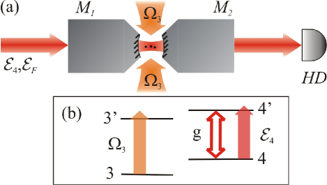
Figure 1: (color online) Schematic of our experiment. Cs atoms are loaded into an intracavity FORT ($\mathcal{E}_{F}$) by way of the transverse cooling field $\Omega_{3}$ and the cavity probe field $\mathcal{E}_{4}$. The transmitted $\mathcal{E}_{4}$ field is directed to a heterodyne detector (HD), allowing real-time determination of intracavity atom number.

In this Letter we report measurements in which the number of atoms trapped inside an optical cavity is observed in real time. After initial loading of the intracavity dipole trap with $\bar{N}\approx 5$ atoms, the decay of atom number $N\geq 3\rightarrow 2\rightarrow 1\rightarrow 0$ is monitored by way of changes in the transmission of a near-resonant probe beam, with the transmitted light exhibiting a cascade of “stairsteps” as successive atoms leave the trap. After the probabilistic loading stage, the time required for the determination of a particular atom number $N=1,2,3$ is much shorter than the mean interval over which the $N$ atoms are trapped. Hence, a precise number of intracavity atoms can be prepared for experiments in QIS, for which the timescales $(g^{-1}\approx 10^{-8}~{}\mathrm{s})\ll(\tau\approx 3~{}\mathrm{s}$), where $\tau$ is the atomic trapping time trapping03 and $\hbar g$ is the atom-field interaction energy. In the present case, the atom number is restricted to $N\lesssim 3$, but the novel detection scheme that we have developed may enable extensions to moderately larger atom numbers $N\lesssim 10$.

As illustrated in Fig. 1, our experiment combines laser cooling, state-insensitive trapping, and strong coupling in cavity QED, as were initially achieved in Ref. trapping03 . A cloud of Cs atoms is released from a magneto-optical trap (MOT) several $\mathrm{mm}$ above the cavity, which is formed by the reflective surfaces of mirrors $(M_{1},M_{2})$ . Several atoms are cooled and loaded into an intracavity far-off-resonance trap (FORT) and are thereby strongly coupled to a single mode of the cavity. The maximum single-photon Rabi frequency $2g_{0}$ for one atom is given by $g_{0}/2\pi=24~{}\mathrm{MHz}$, and is based on the reduced dipole moment for the $6S_{1/2},F=4\rightarrow 6P_{3/2},F^{\prime}=4^{\prime}$ transition of the $D2$ line in Cs at $\lambda_{0}=852.4~{}\mathrm{nm}$. Decay rates for the $6P_{3/2}$ atomic excited states and the cavity mode at $\omega_{0}=2\pi c/\lambda_{0}$ are $\gamma/2\pi=2.6~{}\mathrm{MHz}$ and $\kappa/2\pi=4.2~{}\mathrm{MHz}$, respectively. The fact that $g_{0}\gg(\kappa,\gamma)$ places our system in the strong coupling regime of cavity QED kimble98 , giving critical atom and photon numbers $n_{0}\equiv\gamma^{2}/(2g_{0}^{2})\approx 0.0057$, $N_{0}\equiv 2\kappa\gamma/g_{0}^{2}\approx 0.037$.

The cavity is independently stabilized and tuned such that it supports $TEM_{00}$ modes simultaneously resonant with both the $F=4\rightarrow F^{\prime}=4^{\prime}$ atomic transition at $\lambda_{0}$ and our FORT laser at $\lambda_{F}=935.6~{}\mathrm{nm}$, giving a length $l_{0}=42.2~{}\mathrm{\mu m}$. A weak probe laser $\mathcal{E}_{4}$ excites the cavity mode at $\lambda_{0}$ with the cavity output directed to detector HD, while a much stronger trapping laser $\mathcal{E}_{F}$ drives the mode at $\lambda_{F}$. In addition, the region between the cavity mirrors is illuminated by two orthogonal pairs of counter-propagating cooling beams in the transverse plane (denoted $\Omega_{3}$). Atoms arriving in the region of the cavity mode are exposed to the $(\mathcal{E}_{4},\mathcal{E}_{F},\Omega_{3})$ fields continuously, with a fraction of the atoms cooled and loaded into the FORT by the combined actions of the $\mathcal{E}_{4}$ and $\Omega_{3}$ fields trapping03 . For all measurements, the cavity detuning from the $4\rightarrow 4^{\prime}$ atomic resonance is $\Delta_{C}=0$. The detuning of the $\mathcal{E}_{4}$ probe from the atom-cavity resonance is $\Delta_{4}=+4~{}\mathrm{MHz}$, and its intensity is set such that the mean intracavity photon number $\bar{n}=0.02$ with no atoms in the cavity. The detuning of the $\Omega_{3}$ transverse cooling field is $\Delta_{3}=+25~{}\mathrm{MHz}$ from the $F=3\rightarrow F^{\prime}=3^{\prime}$ resonance, and its intensity is about $I_{3}\approx 4\times 10^{1}~{}\mathrm{mW/cm^{2}}$.

The field $\mathcal{E}_{F}$ that drives the standing-wave, intracavity FORT is linearly polarized, resulting in nearly equal ac-Stark shifts for all Zeeman sublevels of the $F=3,4$ hyperfine ground states of the $6S_{1/2}$ manifold corwin99 . The peak value of the trapping potential is $-U_{0}/h=-47~{}\mathrm{MHz}$, giving a trap depth $U_{0}/k_{B}=2.2~{}\mathrm{mK}$ . A critical characteristic of the FORT is that all states within the $6P_{3/2}$ excited manifold likewise experience a trapping shift of roughly $-U_{0}$ (to within $\approx\pm 15\%$) katori99 ; ido00 ; kimble99 ; trapping03 , which enables continuous monitoring of trapped atoms in our cavity and avoids certain heating effects.

Figure 2(a) displays a typical record of the heterodyne current $i(t)$ resulting from one instance of FORT loading. Here, the current $i(t)$ is referenced to the amplitude of the intracavity field $|\langle\hat{a}\rangle|$ by way of the known propagation and detection efficiencies. The initial sharp drop in $|\langle\hat{a}(t)\rangle|$ around $t=0$ results from atoms that are cooled and loaded into the FORT by the combined action of the $(\mathcal{E}_{4},\Omega_{3})$ fields trapping03 . Falling atoms are not exposed to $\mathcal{E}_{4}$ until they reach the cavity mode, presumably leading to efficient trap loading for atoms that arrive at a region of overlap between the standing waves at $(\lambda_{0},\lambda_{F})$ for the $(\mathcal{E}_{4},\mathcal{E}_{F})$ fields. Trap loading always occurs within a $\pm 10~{}\mathrm{ms}$ window around $t=0.025~{}\mathrm{s}$ (relative to $t=0$ in Fig. 2(a)). This interval is determined using separate measurements of the arrival time distribution of freely falling atoms in the absence of the FORT mabuchi96 ; ye99 .

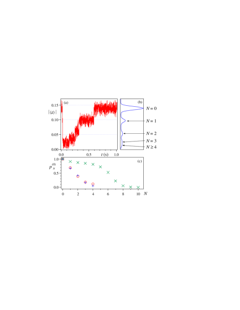
Figure 2: (color online) (a) A typical detection record in which several ($N>4$) atoms are loaded into the trap. Heterodyne detection bandwidth is $1~{}\mathrm{kHz}$. (b) Histogram of 500 such traces, binned with respect to the heterodyne signal $|\langle\hat{a}\rangle|$. A digital low-pass filter of bandwidth $100~{}\mathrm{Hz}$ is applied to each trace prior to the computation of the histogram. (c) Comparison of the model prediction for $p_{0}^{(N)}(y=0.5)$ ($+$) with the measured positions of the histogram peaks in (b) ($\bigcirc$). Also shown ($\times$) is $p_{0}^{(N)}(y=0.1)$ to indicate the possibility to detect specific atom numbers for larger $\bar{N}$.

Subsequent to this loading phase, a number of remarkable features are apparent in the trace of Fig. 2(a), and are consistently present in all the data. The most notable characteristic is the fact that the transmission versus time consists of a series of flat “plateaus” in which the field amplitude is stable on long timescales. Additionally, these plateaus reappear at nearly the same heights in all repeated trials of the experiment, as is clearly evidenced by the histogram of Fig. 2 (b). We hypothesize that each of these plateaus represents a different number $N$ of trapped atoms coupled to the cavity mode, as indicated by the arrows in Fig. 2.

Consider first the one-atom case, which unexpectedly exhibits relatively large transmission and small variance. For fixed drive $\mathcal{E}_{4}$, the intracavity field is a function of the coupling parameter $g^{(i,f)}(\mathbf{\ r})=g_{0}G_{i,f}\sin(k_{0}z)\exp(-2\rho^{2}/w_{0}^{2})$ where $\rho$ is the transverse distance from the cavity axis ($z$), $k_{0}=2\pi/\lambda_{0}$, and $G_{i,f}$ relates to the Clebsch-Gordan coefficient for particular initial and final states $(i,f)$ within the $F=4,F^{\prime}=4^{\prime}$ manifolds hood98 ; puppe03 . Variations in $g$ as a function of the atom’s position $\mathbf{r}$ and internal state might reasonably be expected to lead to large variations of the intracavity field, both as a function of time and from atom to atom.

However, one atom in the cavity produces a reasonably well-defined intracavity intensity $I\propto|\langle\hat{a}\rangle|^{2}$ due to the interplay of two effects. The first is that for small probe detunings $\Delta_{4}$, the intracavity intensity $I_{1}$ for one atom is suppressed by a factor $f$ relative to the empty-cavity intensity $I_{0}$, where for weak excitation, $f\approx 4C_{1}^{2}\gg 1$ with $C_{1}=g^{2}/2\kappa\gamma$. A persistent, strongly reduced transmission thereby results, since the condition $[C_{1}^{(i,f)}(\mathbf{r})]^{2}\gg 1$ is robust to large fluctuations in atomic position $\mathbf{r}$ and internal state. The second effect is that the $F=4\leftrightarrow F^{\prime}=4^{\prime}$ transition cannot be approximated by a closed, two-level system, since the $F^{\prime}=4^{\prime}$ excited states decay to both $F=3,4$ hyperfine ground levels. As illustrated in Fig. 1(b), an atom thus spends a fraction $q$ of its time in the cavity QED manifold $(4,4^{\prime})$, and a fraction $p\approx 1-q$ in the $(3,3^{\prime})$ manifold. In this latter case, the effective coupling is negligible ($C_{1}^{eff}\approx 4\times 10^{-4})$, leading to an intensity that approximates $I_{0}$. Hence, the intracavity intensity as a function of time $I(t)$ should have the character of a random telegraph signal switching between levels $(I_{0},I_{1})$, with dwell times determined by $(\mathcal{E}_{4},\Omega_{3})$, which in turn set $p$ dark . Since $(\mathcal{E}_{4},\Omega_{3})$ drive their respective transitions near saturation, the timescale $\tau_{P}\sim 1~{}\mu\mathrm{s}$ for optical pumping from one manifold to another is much faster than the inverse detection bandwidth $(1/2\pi B)\approx 160~{}\mu\mathrm{s}$. The fast modulation of the intracavity intensity due to optical pumping processes thereby gives rise to an average detected signal corresponding to intensity $\bar{I}_{1}\approx pI_{0}+qI_{1}\approx pI_{0}$ for $I_{1}\ll I_{0}$.

This explanation for the case of $1$ atom can be extended to $N$ intracavity atoms to provide a simple model for the “stairsteps” evidenced in Fig. 2(a). For $N$ atoms, the intracavity intensity should again take the form of a random telegraph signal, now switching between the levels $(I_{0},I_{k})$, with high transmission $I_{0}$ during intervals when all $N$ atoms happen to be pumped into the $(3,3^{\prime})$ manifold, and with low transmission $I_{k}\leq I_{1}$ anytime that $1\leq k\leq N$ atoms reside in the $(4,4^{\prime})$ manifold, where $I_{k}\sim I_{1}/k^{2}$ for weak excitation with $\Delta_{C}=\Delta_{4}=0$. The intracavity intensities $\{I_{k}\}$ determine the transition rates $\{\gamma_{k\rightarrow k-1}\}$ between states with $k$ and $k-1$ atoms in the $(4,4^{\prime})$ manifold, while $\Omega_{3}$ determines $\{\gamma_{k-1\rightarrow k}\}$ for $k-1\rightarrow$ $k$ via transitions from the $(3,3^{\prime})$ manifold. For the hierarchy of states $k=0,1,\ldots,N$ with transition rates $\{\gamma_{k\rightarrow k-1,}\gamma_{k-1\rightarrow k}\}$, it is straightforward to determine the steady-state populations $p_{k}^{(N)}$. With the physically motivated assignments $\gamma_{k-1\rightarrow k}=\gamma_{0\rightarrow 1}$ independent of $k$ and $\gamma_{k\rightarrow k-1}=\gamma_{1\rightarrow 0}/k^{2}$ corresponding to $I_{k}\sim I_{1}/k^{2}$, we find that $p_{0}^{(N)}=1/\sum_{k=0}^{N}(k!)^{2}y^{k}$, where $y\equiv\gamma_{0\rightarrow 1}/\gamma_{1\rightarrow 0}$. Hence, for $I_{k}\ll I_{0}$, the prediction for the average intensity is $\bar{I}_{N}\approx p_{0}^{(N)}I_{0}$, which leads to a sequence of plateaus of increasing heights $\bar{I}_{N+1}\rightarrow\bar{I}_{N}\rightarrow\bar{I}_{N-1}$ as successive atoms are lost from the trap $N+1\rightarrow N\rightarrow N-1$.

Figure 2(c) compares the prediction of this simple model with the measured values of peak positions in (b). The only adjustable parameter is the value $y=0.5$, resulting in reasonable correspondence between the model and the measurements. Also shown are values $p_{0}^{(N)}$ for $y=0.1$ to indicate that it might be possible to enhance the resolution for a particular range of atom number by framing a given few values $N_{1},N_{1}\pm 1$ in the transition region $p_{0}^{(N_{1})}\approx 0.5$, where $N_{1}\approx 6$ in (c). This could be accomplished by adjusting the relative strengths of the $(\mathcal{E}_{4},\Omega_{3})$ fields and hence $y$.

Although our simple model accounts for the qualitative features in Fig. 2, a quantitative description requires a considerably more complex analysis based upon the full master equation for $N$ intracavity atoms, including the multiple Zeeman states and atomic motion through the polarization gradients of the $\Omega_{3}$ beams. We have made initial efforts in this direction boozer04 for one atom, and are working to extend the treatment to $N\geq 2$ atoms.

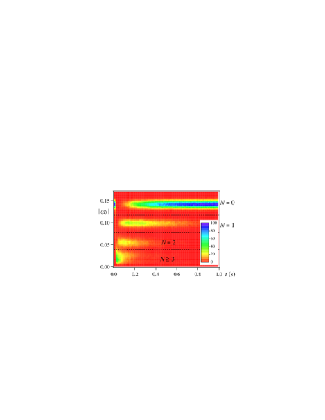
Figure 3: (color online) Histogram of 500 traces such as the one in Fig. 2(a), binned with respect to both signal strength $|\langle\hat{a}\rangle|$ and time $t$. The signals are filtered first as in Fig. 2(b).

Beyond these considerations, additional evidence that the plateaus in Fig. 2 correspond to definite atom numbers is provided by Fig. 3. Here, the data recorded for the probe transmission have been binned not only with respect to the value of $|\langle\hat{a}\rangle|$ as in Fig. 2(b), but also as a function of time. Definite plateaus for $|\langle\hat{a}\rangle|$ are again apparent, but now their characteristic time evolution can be determined. The critical feature of this plot is that the plateaus lying at higher values of $|\langle\hat{a}\rangle|$ correspond to times later in the trapping interval, in agreement with the expectation that $N$ should always decrease with time beyond the small window of trap loading around $t=0.025~{}\mathrm{s}$. This average characteristic of the entire data set supports our hypothesis that the plateaus in $|\langle\hat{a}\rangle|$ correspond to definite intracavity atom numbers $N$, as indicated in Figs. 2 and 3. Moreover, none of the 500 traces in the data set includes a downward step in transmission after the initial trap loading.

To examine the dynamics of the trap loss more quantitatively, we consider each atom number individually by integrating the “plateau” regions along the $|\langle\hat{a}(t)\rangle|$ axis for each time $t$. The dashed horizontal lines in Fig. 3 indicate the boundaries chosen to define the limits of integration for each value of $N$. We thereby obtain time-dependent “populations” $\Phi_{N}(t)$ for $N=0,1,2$, and $\Phi_{\geq 3}(t)=\sum_{N=3}^{\infty}\Phi_{N}(t)$, which are plotted in Fig. 4(a). To isolate the decay dynamics from those of trap loading, we plot the data beginning at $t_{0}=0.034~{}\mathrm{s}$ with respect to the origin in Figs. 2(a) and 3. The qualitative behavior of these populations is sensible, since almost all trials begin with $N\geq 3$, eventually decaying to $N=2,1,0$.

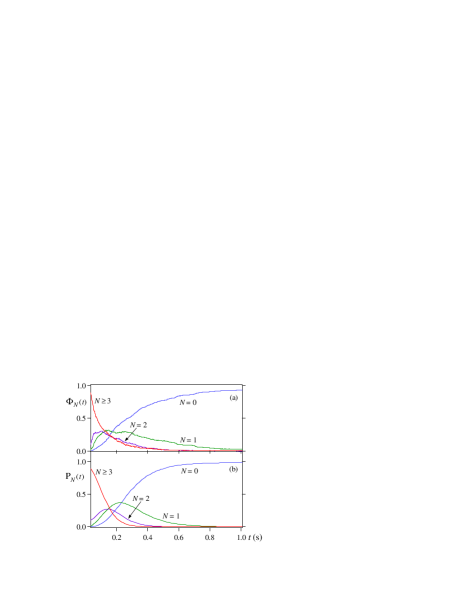
Figure 4: (color online) (a) Experimental results for the time evolution of the $N$-atom populations $\Phi_{N}(t)$, which are normalized such that their sum is approximately unity throughout the interval shown. (b) The results of a simple model calculation $P_{N}(t)$ are fit to the data $\Phi_{N}(t)$ with one free parameter, the single atom decay rate $\Gamma$.

The quantities $\Phi_{N}(t)$ are approximately proportional to the fraction of experimental trials in which $N$ atoms were trapped at time $t$, so long as the characteristic duration $\Delta t_{N}$ of each plateau far exceeds the time resolution of the detection. If the bandwidth is too low, transient steps no longer represent a negligible fraction of the data, as is the case for transitions between the shortest-lived levels (e.g., $N=3\rightarrow 2$). We estimate that this ambiguity causes uncertainties in $\Phi_{N}$ at the $5-10\%$ level.

Also shown in panel (b) of Fig. 4 is the result of a simple birth-death model for predicting the time evolution of the populations, namely $\dot{P}_{N}(t)=-\Gamma(NP_{N}(t)-(N+1)P_{N+1}(t))$, where $P_{N}(t)$ represents the probability of $N$ atoms in the trap. The main assumption of the model is that there is one characteristic decay rate $\Gamma$ for trapped atoms, and that each atom leaves the trap independently of all others. Initial conditions for $N=0$, $1$ and $2$ for the solution presented in Fig. 4(b) are obtained directly from the experimental data after trap loading, $\Phi_{N}(t_{0})$. Since the plateaus for higher values of $N$ are not well resolved, we use a Poisson distribution for $N\geq 3$. The mean $\mu=5.2$ is obtained by solving $\sum_{N=3}^{\infty}e^{-\mu}\mu^{N}/N!=\Phi_{N\geq 3}(t_{0})$. Given these initial conditions, we perform a least-squares fit of the set of analytic solutions $\{P_{N}(t)\}$ to the set of experimental curves $\{\Phi_{N}(t)\}$ with $\Gamma$ the only free parameter, resulting in the curves in Fig. 4(b) with $\Gamma=8.5~{}\mathrm{s}^{-1}$. Although there is reasonable correspondence between Figs. 4 (a) and (b), $\Phi_{N}(t)$ evolves more rapidly than does $P_{N}(t)$ at early times, and yet the data decay more slowly at long times. This suggests that there might be more than one timescale involved, possibly due to an inhomogeneity of decay rates from atom to atom or to a dependence of the decay rate on $N$. We have observed non-exponential decay behavior in other measurements of single-atom trap lifetimes, and are working to understand the underlying trap dynamics.

Our experiment represents a new method for the real-time determination of the number of atoms trapped and strongly coupled to an optical cavity. We emphasize that an exact number $N=1$ to $3$ coupled atoms can be prepared in our cavity within $\approx 200~{}\mathrm{ms}$ from the release of the MOT. Although the trap loading is not deterministic, $N$ can be measured quickly compared to the subsequent trapping time $\tau\approx 3~{}\mathrm{s}$ trapping03 . These new capabilities are important for the realization of various protocols in quantum information science, including probabilistic protocols for entangling multiple atoms in a cavity duan03 ; hong02 ; sorensen03 . Although our current investigation has centered on the case of small $N\leq 3$, there are reasonable prospects to extend our technique to higher values $N\lesssim 10$ as, for example, by way of the strategy illustrated in Fig. 2(c). Moreover, the rate at which we acquire information about $N$ can be substantially increased from the current value $\kappa|\langle\hat{a}\rangle|^{2}\sim 10^{5}/$s toward the maximum rate for optical information $g^{2}/\kappa\gtrsim 10^{8}/$s, which can be much greater than the rate for fluorescent imaging set by $\gamma$ hood00 .

References

- (1) H. J. Kimble, Physica Scripta T76, 127 (1998).
- (2) J. McKeever et al., Science, published online 26 February 2004; 10.1126/science.1095232.
- (3) C. J. Hood et al., Science 287, 1447 (2000).
- (4) H. Mabuchi and A. C. Doherty, Science 298, 1372 (2002).
- (5) T. Pellizzari et al., Phys. Rev. Lett. 75, 3788 (1995).
- (6) J. I. Cirac et al., Phys. Rev. Lett. 78, 3221 (1997).
- (7) H.-J. Briegel et al., in The Physics of Quantum Information, edited by D. Bouwmeester, A. Ekert and A. Zeilinger, p. 192.
- (8) J. Ye, D. W. Vernooy and H. J. Kimble, Phys. Rev. Lett. 83, 4987 (1999).
- (9) J. McKeever et al., Phys. Rev. Lett. 90, 133602 (2003).
- (10) P. Maunz et al., Nature (London) 428, 50 (2004).
- (11) L. M. Duan and H. J. Kimble, Phys. Rev. Lett. 90, 253601 (2003).
- (12) J. Hong and H.-W. Lee, Phys. Rev. Lett. 89, 237901.
- (13) A. S. Sørensen and K. Mølmer, Phys. Rev. Lett. 90, 127903 (2003).
- (14) G. R. Guthörlein et al., Nature (London) 414, 49 (2001); A. B. Mundt et al., Phys. Rev. Lett. 89, 103001 (2002).
- (15) K. L. Corwin et al., Phys. Rev. Lett. 83, 1311 (1999).
- (16) H. Katori et al., J. Phys. Soc. Jpn. 68, 2479 (1999).
- (17) T. Ido et al., Phys. Rev. A 61, 061403 (2000).
- (18) H. J. Kimble et al. in Laser Spectroscopy XIV, edited by R. Blatt et al. (World Scientific, Singapore, 1999), p. 80.
- (19) H. Mabuchi et al., Opt. Lett. 21, 1393 (1996).
- (20) C. J. Hood et al., Phys. Rev. Lett. 80, 4157 (1998).
- (21) T. Puppe et al., Opt. Lett. 28, 46 (2003).
- (22) Fluctuations in intracavity intensity can also arise from optical pumping into dark states. Although the probe field is linearly polarized with dark state , independent measurements indicate the presence of significant Zeeman splittings MHz for , partially arising from residual ellipticity of the FORT field trapping03 ; corwin99 and from uncompensated stray magnetic fields. Moreover, an atom moving at travels through the polarization gradients of the field in , ensuring rapid pumping from dark states in the ground level. Occupation of dark states for extended periods is thereby precluded, as is supported by detailed Monte-Carlo simulations for boozer04 .
- (23) A. D. Boozer et al., Phys. Rev. A (available at http://arXiv.org/abs/quant-ph/0309133).