Entangled states of light

Abstract

These notes are more or less a faithful representation of my talk at the Workshop on “Quantum Coding and Quantum Computing” held at the University of Virginia. As such it is an introduction for non-physicists to the topics of the quantum theory of light and entangled states of light. In particular, I discuss the photon concept and what is really entangled in an entangled state of light (it is not the photons!). Moreover, I discuss an example that highlights the peculiar behavior of entanglement in an infinite-dimensional Hilbert space.

I Light

Thanks to a certain class of T-shirts T we all know that light is described by Maxwell’s equations. These equations determine how the electric and magnetic fields vary in space and time, given electric currents and charges. Fortunately, even if there are no sources, that is, no currents and no charges, there are still nontrivial solutions. It is those solutions that describe light waves. One way to express such a light wave is to write down the electric field vector as a function of position $\vec{r}$ and time $t$,

$$\vec{E}(\vec{r},t)=\vec{\epsilon}\exp i\big{(}\vec{k}\cdot\vec{r}-\omega t\big{)}+{\rm complex}\;{\rm conjugate}.$$ (1)

This wave corresponds to a monochromatic plane wave with frequency $\omega$, propagating in the direction of $\vec{k}$, and with a polarization $\vec{\epsilon}$. These quantities are not independent as they satisfy

$$|\vec{k}|c=\omega;\,\,\vec{k}\cdot\vec{\epsilon}=0.$$ (2)

Here $c$ is the speed of, what else, light. The general solution to the source-free Maxwell equations is a sum (or an integral, depending on whether we allow $\vec{k}$ to take continuous values) of plane waves, according to

$$\vec{E}(\vec{r},t) = \sum_{\vec{k}}\sum_{\vec{\epsilon}\perp\vec{k}}A_{\vec{k},\vec{\epsilon}}\,\vec{\epsilon}\exp i\big{(}\vec{k}\cdot\vec{r}-\omega t\big{)}$$ (3)

$$+{\rm complex}\;{\rm conjugate},$$

where $A_{\vec{k},\vec{\epsilon}}$ are arbitrary complex coefficients, called amplitudes, that determine the intensity of the light beam.

The Maxwell equations and hence its solutions (3) are “classical”, as they do not describe any quantum effects. So, what changes if we are to use a quantum theory of light? Some may think that the frequency $\omega$ becomes quantized, that is, takes on only discrete values. Others may think the polarization vector $\vec{\epsilon}$ becomes a quantum object. Pessimists may think that the Maxwell equations are no longer valid and perhaps polarization and frequency are no longer well defined. But none of these expectations are correct. What really happens when one quantizes the electromagnetic field is the following: Just as position and momentum of a particle become operators acting on some complex Hilbert space when one quantizes the particle, so do the electric (and magnetic) fields become operators in a quantum theory of light. It turns out that the Maxwell equations keep in fact the same form. So, the solutions (3) are also still valid, except that “complex conjugate” becomes “Hermitian conjugate.”

The difference with the classical solutions (3) is that the amplitudes $A_{\vec{k},\vec{\epsilon}}$ become operators. We typically write the amplitude as the product of a number (with the dimension of an electric field), and a dimensionless operator $a_{\vec{k},\vec{\epsilon}}$. For each value of $(\vec{k},\vec{\epsilon})$, called a mode, there is such an operator $a$ (leaving out the subscripts for ease of notation). That operator acts on a complex Hilbert space. In the case of the electromagnetic field, that Hilbert space is infinite-dimensional. It is spanned by states $|n\rangle$ for $n=0,1,2\ldots$, and the operator $a$ acts as

$$a|n\rangle=\sqrt{n}|n-1\rangle.$$ (4)

The number $n$ is interpreted as the number of photons in the corresponding mode. Thus the state $|2\rangle$ is a state with two photons in a particular mode. The operator $a$ annihilates one photon, and is called the annihilation operator. Similarly, the Hermitian conjugate operator, $a^{\dagger}$ acts as

$$a^{\dagger}|n\rangle=\sqrt{n+1}|n+1\rangle,$$ (5)

and is called the creation operator. The fact that the number states $|n\rangle$ start with $n=0$ is not just a convenient convention: Eq. (4) shows that $a$ acting on the state $|0\rangle$ gives nothing, zero, not even a state. We cannot have a state with $-1$ photons.

For later use we note that if we define $N=a^{\dagger}a$, we have in fact managed to define the number operator,

$$N|n\rangle=n|n\rangle,$$ (6)

that counts the number of photons in a mode.

I.1 Entangled states of light

To make an entangled state of light we need (at least) two modes. Suppose we have two modes, denoted by $A$ and $B$. Modes $A$ and $B$ may correspond to modes with the same frequency and the same wave vector, but different (orthogonal) polarizations. Or they may have the same polarization and the same frequency, but propagate in a different (not necessarily orthogonal) direction. In any case, the Hilbert space $H_{A,B}$ associated with the two modes is the tensor product $H_{A,B}=H_{A}\otimes H_{B}$ of the Hilbert spaces of each of the modes.

Let us look at a simple example of a state in $H_{A,B}$:

$$|\Psi\rangle_{A,B}=[|0\rangle_{A}|1\rangle_{B}+|1\rangle_{A}|0\rangle_{B}]/\sqrt{2}.$$ (7)

Although properly we should have written $|0\rangle_{A}\otimes|1\rangle_{B}$ etc., we used here the physicists’ convention to be lazy. This state is entangled because it cannot be written as a product of two states of the modes $A$ and $B$. Thus neither mode is in a well-defined pure state of itself. Loosely speaking, we could say there is one photon, and it is either in mode $A$ or in mode $B$. This way of speaking misses some essential points though. The state (7) expresses more than just a classical joint probability distribution to find the photon in modes $A$ and $B$. In particular, if modes $A$ and $B$ are spatially separated, then the statistics of measurement outcomes on the state (7) can in general not be obtained from any classical joint probability distribution without superluminal communication. Since physicists don’t like superluminal communication, this expresses a serious difference between quantum and classical mechanics. [Note that this does not imply that entanglement can be used for superluminal communication, it is just that a classical local model cannot explain quantum mechanics.] This basically is the content of Bell’s theorem. I refer to Bell’s book bell for the details.

I.2 What is entangled?

We found that the state (7) is entangled. But what is entangled with what? One might think photons are entangled with each other. That is indeed not the most stupid answer one can give, as after all light consists of photons. Nevertheless, it is not the photons that are entangled. In fact, there is only one photon in the state (7). Instead, modes $A$ and $B$ are entangled with each other. The number of photons just determines the states of the modes.

Now, however, this leads to a slight problem. After all, nobody tells us how to define our modes. We can take any complete set of functions to expand our electric field in, as in Eq. (3), and to each member of that set corresponds a mode. So unlike in the case of, say, atoms in a trap, we are more or less free to define what we mean by our systems. With atoms in a trap, the atoms are clearly the systems, but for light modes it is a lot less clear. For instance, if modes $A$ and $B$ correspond to horizontal and vertical polarization, respectively (with all other mode variables, the wave vector and the frequency, the same), then the entangled state (7) turns out to be equal to a state with one diagonally polarized photon. Formally, by defining new annihilation operators $a^{\prime}_{\pm}=(a_{A}\pm a_{B})/\sqrt{2}$, we find that there is one photon in mode ${}^{\prime}+^{\prime}$ and no photons in mode ${}^{\prime}-^{\prime}$. However, that state we would never call entangled.

On the other hand, suppose modes $A$ and $B$ correspond to spatially separated modes, mode $A$ is here, mode $B$ is there. The $\pm$ modes can theoretically still be defined. However, in practice the modes “here plus there” and “here minus there” are useless. In particular, noone would know how to directly measure a photon in such a mode. (Of course, one can always indirectly measure such modes by recombining the modes so that they end up in the same location. But that’s cheating as one explicitly changes the modes and thereby the entanglement.) Thus, when the modes $A$ and $B$ are spatially separated no redefinitions of those modes are useful. So we decree that it makes sense to talk unambiguously about entanglement between two modes $A$ and $B$ only if the modes are spatially separated. If the modes are in the same location we do allow redefinitions of the modes and thereby of the entanglement.

I.3 Some remarks

The importance attached to nonlocality for the issue of defining entanglement is consistent with several other results: first of all, there is above-mentioned Bell’s theorem. Second, there has been a lot of interest in relativistic aspects of entanglement of both light and particles, such as electrons. One conclusion scudo , in particular, is that the entanglement between different degrees of freedom of one particle (namely, the spin and the momentum) is not Lorentz-invariant. That is, the amount of entanglement present within that one particle depends on the velocity of the observer. The reason is that different observers don’t agree on what the spin and momentum degrees are. This is similar to having different observers disagreeing on how the modes of the electromagnetic field are defined. When talking about two particles in different positions, no such problems arise. Third, it has been shown spreeuw that many quantum properties of light, even including entanglement, can be simulated by using just classical light beams. However, this is only so if the entanglement is not nonlocal.

The point that entanglement is between modes and not between photons was made in several different papers pz ; em , all coming out at roughly the same time. Apart from making that same point, the papers do have different ideas otherwise. In particular, my own attempt em at a paper discusses by how much redefinitions of modes can change the entanglement. For example, in the simple state (7), the smallest and largest possible amounts of entanglement one can get are just zero, and one unit of entanglement, respectively. There are other simple examples where the entanglement cannot be transformed away completely, and also examples where the maximum entanglement possible is probably more than what one would have expected at first and even second glance.

Finally, I also note that the importance of what can actually be measured for the definition of entanglement was discussed in a more general and more precise context in barnum . This was also discussed at the Workshop by Lorenza Viola.

II Entangled coherent states

This Section serves a number of purposes. First, it shows an explicit nontrivial (as opposed to (7)) example of an entangled state. Second, that example will display some curious behavior that is known to occur in principle in infinite-dimensional Hilbert spaces, but for which there was no more or less practical example known.

The easiest way to generate a light beam with nice quantum properties is to switch on a laser. The quantum state of the light beam is a so-called coherent state [disregarding some subtleties that are of no interest here]. For any complex number $\alpha$ it is defined as

$$|\alpha\rangle:=\exp(-|\alpha|^{2}/2)\sum_{n=0}^{\infty}\frac{\alpha^{n}}{\sqrt{n!}}|n\rangle,$$ (8)

in terms of the number states $|n\rangle$. The easiest way to produce a nontrivial state of two modes, is to take a laser beam and split it on a beam splitter. Annoyingly, though, one can never get an entangled state out of these two easy operations. If we split two coherent states on a beam splitter we just get two new coherent states with different amplitudes, but nothing more. In fact, more generally speaking, with linear optics one cannot create entanglement from coherent states. The reason is that all linear optics elements just lead to linear transformations of operators $a_{i}$ of modes $i$. Namely, the general transformation is of the form

$$a^{\prime}_{j}=\sum_{i}U_{ij}a_{j},$$ (9)

with $U_{ij}$ a unitary matrix. Since a coherent state (8) is an eigenstate of $a$, and since the transformations (9) can only transform eigenstates of the operators $a_{i}$ into eigenstates of new mode operators $a^{\prime}_{j}$, coherent states are always transformed into coherent states.

Thus, in order to create entanglement from a coherent state one needs nonlinear optics. One particular type of nonlinearity I consider here is the Kerr nonlinearity. It is characterized by a Hamiltonian of the form

$$H=\hbar\chi a^{\dagger 2}a^{2},$$ (10)

where $\hbar$ is Planck’s constant. The Hamiltonian determines the evolution in time of any state, with the evolution operator as a function of time $t$ given by

$$U(t)=\exp(-itH/\hbar).$$ (11)

Starting from a coherent state $|\alpha\rangle$ at time $t=0$ the state evolves thus as

$$|\psi(t)\rangle=\exp(-itH/\hbar)|\alpha\rangle.$$ (12)

The evolution operator can be rewritten in terms of the number operator defined in (6),

$$U(\tau)=\exp(-i\tau a^{\dagger 2}a^{2})=\exp(-i\tau N(N-1)),$$ (13)

where $\tau=\chi t$ is a dimensionless time. The operator $U$ becomes periodic in $N$ with period $M$ (that is, it becomes invariant under $N\rightarrow N+M$) at times $\tau=\pi/M$ if $M$ is an odd integer. This implies one can write down Fourier series as follows [following Ref. tara ]

$$\exp\big{(}\frac{-i\pi}{M}N(N-1)\big{)}=\sum_{q=0}^{M-1}f_{q}^{(o)}\exp\big{(}\frac{-2i\pi q}{M}N\big{)}.$$ (14)

Similarly, for even values of $M$ one has

$$\exp\big{(}\frac{-i\pi}{M}(N+M)^{2}\big{)}=\exp\big{(}\frac{-i\pi}{M}N^{2}\big{)},$$ (15)

so that we can expand

$$\exp\big{(}\frac{-i\pi}{M}N^{2}\big{)}=\sum_{q=0}^{M-1}f_{q}^{(e)}\exp\big{(}\frac{-2i\pi q}{M}N\big{)}.$$ (16)

The coefficients $f_{q}$ are not explicitly evaluated in Ref. tara , but one can actually derive them (see multi for more details),

$$f_{q}^{(o)} = \frac{1}{\sqrt{M}}\exp\big{(}\frac{\pi iq(q+1)}{M}\big{)}\exp\big{(}\frac{-\pi iK(K+1)}{M}\big{)},$$

$$f_{q}^{(e)} = \frac{1}{\sqrt{M}}\exp\big{(}\frac{\pi iq^{2}}{M}\big{)}\exp(-\pi i/4),$$ (17)

where in the first line $K$ is such that $M=2K+1$ for odd $M$. The expansions (14) and (15) are useful as it becomes easy to calculate the effect of the evolution opertor on a coherent state. The reason is the simple relation

$$\exp(i\phi N)|\alpha\rangle=|\alpha\exp(i\phi)\rangle.$$ (18)

Thus, if one starts with a coherent state at time $\tau=0$, this then immediately leads to the following time evolution under $U$:

$$U(\pi/M)|\alpha\rangle = \sum_{q=0}^{M-1}f_{q}^{(o)}|\alpha\exp(-2\pi iq/M)\rangle$$

$${\rm for}\,\,M\,\,{\rm odd},$$

$$U_{A}(\pi/M)|\alpha\rangle = \sum_{q=0}^{M-1}f_{q}^{(e)}|\alpha\exp(\pi i(1-2q)/M)\rangle$$

$${\rm for}\,\,M\,\,{\rm even}$$ (19)

If one subsequently takes these states and splits them on a 50/50 beamsplitter with the vacuum, the output state is an entangled state of the form

$$|\Phi_{M}\rangle=\sum_{q=0}^{M-1}f_{q}^{(o)}|\beta\exp(-2\pi iq/M)\rangle|\beta\exp(-2\pi iq/M)\rangle,$$ (20)

for $M$ odd with $\beta=\alpha/\sqrt{2}$, and something similar for even $M$.

The state (20) is entangled. A measure for how much entanglement there is in a state of two modes can be obtained after first writing the state in a standard form, the so-called Schmidt-decomposition form. There is a unique (up to some trivial transformations) way to write a bipartite state as

$$|\Psi\rangle=\sum_{q=0}^{M-1}\sqrt{p}_{q}|\psi_{q}\rangle|\phi_{q}\rangle,$$ (21)

where the $p_{q}$ are positive real numbers with $\sum_{q}p_{q}=1$ (so they can be interpreted as probabilities), and with the states $|\psi_{q}\rangle$ for $q=0\ldots M-1$ all orthogonal to each other, and the same for $|\phi_{q}\rangle$. The entanglement is then given by

$$E=-\sum p_{q}\log_{2}p_{q},$$ (22)

which some may recognize as the Shannon entropy of the probability distribution $\{p_{q}\}$. If we have $M$ terms in (21) then the entanglement can at most be $\log_{2}M$. Now the state (20) is almost written in the Schmidt form (21). It is only “almost”, as I had not told you yet that the coherent states are not orthogonal, as can be checked directly from the definition. However, for large values of $|\alpha|$ the different coherent states do become orthogonal, so in that limit the entanglement in the state (20) is $E=\log_{2}M$.

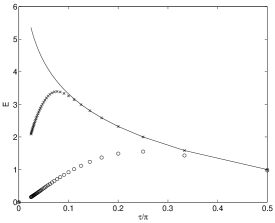
Figure 1: Entanglement for the states (20) as a function of $\tau$, for various values of $|\alpha|^{2}$: $|\alpha|^{2}=1$ for the bottom curve (circles), $|\alpha|^{2}=10$ for the middle curve (crosses), and $|\alpha|^{2}\rightarrow\infty$ for the top curve (solid line).

Now here is a peculiar effect: we get more entanglement with increasing $M$, that is, if we remember we generated this state after a time $\tau=\pi/M$, with decreasing time. So the shorter the nonlinear Hamiltonian (10) acts, the more entanglement we get (and we started with no entanglement). How can this possibly be right? The answer lies hidden in the assumption of large $\alpha$: for increasing $M$ the different coherent states are only orthogonal when $|\alpha/M|\gg 1$. So, with increasing $M$ one needs ever larger values of $\alpha$. Now the energy in a coherent state is proportional to $|\alpha|^{2}$, so the energy needed to make $\log_{2}M$ units of entanglement grows as $M^{2}$. Now it is known wehrl that entanglement in infinite dimensions is not a continuous function of the state. But, if one restricts oneself to states with an upper bound on the total energy, then that function is continuous. Here too, the peculiar behavior of entanglement disappears when we fix the value of $\alpha$ and then calculate the entanglement as a function of time $\tau$. For small $\tau$ the entanglement will be small: the above-mentioned argument that the entanglement should be large does not hold for fixed $\alpha$ as the coherent states become very non-orthogonal for large $M$. This is illustrated in Fig. 1, where the entanglement as a function of $\tau$ is plotted for 2 different values of $\alpha$ together with the maximum possible amount of entanglement (only reached for $|\alpha|\rightarrow\infty$).

A final question to be answered is the following. Even though we know now that there is no real contradiction arising from the fact that in principle a large amount of entanglement can be created after a short interaction time, one may wonder whether that effect can be useful for creating lots of entanglement without being bothered too much by decoherence. After all, a shorter interaction time implies in general less decoherence. If you fund my research, please stop reading now. Unfortunately, there is a catch. One only creates those large amounts of entanglement in short times if the amplitude $\alpha$ is large. That in turn leads to more decoherence. The more photons there are in a state, the easier they are lost. A more precise analysis shows that the increasing decoherence indeed seriously counteracts the potential increase of entanglement. Thus, it seems one is not better off using very short interaction times to create entanglement with the Kerr interaction. On that happy note, I end.

III Acknowledgments

I thank Olivier Pfister for having been a great host and Karen Klintworth for having taken care of all the annoying but important details.

References

- (1) www.twobarkingdogs.com. And God said, Let there be Light.
- (2) J.S. Bell, Speakable and unspeakable in quantum mechanics, Cambridge University Press, 1993.
- (3) A. Peres, P.F. Scudo, and D.R. Terno, Phys. Rev. Lett. 88, 230402 (2002).
- (4) R.J.C. Spreeuw, Found. Phys. 28, 361 (1998); Phys. Rev. A 63, 062302 (2001).
- (5) P. Zanardi, Phys. Rev. A 65, 042101 (2002); Y. Shi, Phys. Rev. A 67, 024301 (2003); V. Vedral, quant-ph/0302040.
- (6) S.J. van Enk, Phys. Rev. A 67, 022303 (2003).
- (7) H. Barnum et al., quant-ph/0305023.
- (8) K. Tara, G.S. Agarwal, and S. Chaturvedi, Phys. Rev. A 47, 5024 (1993).
- (9) S.J. van Enk, Phys. Rev. Lett. 91, 017902 (2003).
- (10) A. Wehrl, Rev. Mod. Phys. 50, 221 (1978); see also J. Eisert, C. Simon, and M.B. Plenio, J. Phys. A 35, 3911 (2002).