Dissipative quantum dynamics with the Surrogate Hamiltonian approach. A comparison between spin and harmonic baths.

Abstract

The dissipative quantum dynamics of an anharmonic oscillator coupled to a bath is studied with the purpose of elucidating the differences between the relaxation to a spin bath and to a harmonic bath. Converged results are obtained for the spin bath by the Surrogate Hamiltonian approach. This method is based on constructing a system-bath Hamiltonian, with a finite but large number of spin bath modes, that mimics exactly a bath with an infinite number of modes for a finite time interval. Convergence with respect to the number of simultaneous excitations of bath modes can be checked. The results are compared to calculations that include a finite number of harmonic modes carried out by using the multi-configuration time-dependent Hartree method of Nest and Meyer, [J. Chem. Phys. 119, 24 (2003)]. In the weak coupling regime, at zero temperature and for small excitations of the primary system, both methods converge to the Markovian limit. When initially the primary system is significantly excited, the spin bath can saturate restricting the energy acceptance. An interaction term between bath modes that spreads the excitation eliminates the saturation. The loss of phase between two cat states has been analyzed and the results for the spin and harmonic baths are almost identical. For stronger couplings, the dynamics induced by the two types of baths deviate. The accumulation and degree of entanglement between the bath modes have been characterized. Only in the spin bath the dynamics generate entanglement between the bath modes.

I Introduction

Modeling quantum many-body systems is a challenging problem. The main obstacle is the exponential growth in complexity with the number of degrees of freedom. Significant simplifications are achieved by partitioning the total system into a primary part and a bath describing the environment Weiss (1999). The idea is to model the primary system explicitly and the bath implicitly, thus minimizing the complexity of the bath to its influence on the primary system. A bath composed of a set of noninteracting harmonic oscillators is the one most widely used. The idea originates from a normal mode analysis combined with a weak system-bath coupling assumption Feynman and Vernon (1963). If the bath is only weakly perturbed by the system, it can be considered linear, and therefore described as a collection of harmonic oscillators. Such a bath is natural for systems interacting with the radiation field Louisell (1990). The harmonic bath model has also been applied to less favorable scenarios such as energy relaxation and dephasing of molecules in the liquid phase or on solids. In these cases a strong coupling or interactions with a low-temperature environment may cause large system-bath correlations, and will therefore result in a failure of the Markovian approximation. To overcome such difficulties in the dynamics of molecules that are in intimate interaction with an environment, an alternative approach termed the Surrogate Hamiltonian Baer and Kosloff (1997) has been developed. The Surrogate Hamiltonian method employs a bath composed of two-level systems that acts as a spin bath Caldeira et al. (1993); Forsythe and Makri (1998); Tsonchev and Pechukas (1999); Prokof’ev and Stamp (2000); Shao and Hänggi (1998).

The concept of the system-bath separation underlines the quantum description of many body dynamics. The origins of the spin and harmonic baths are different. The harmonic bath is closely related to a normal mode decomposition. Once this is done the spectral density function is able to completely determine the relaxation dynamics. From a computational point of view the determination of the spectral density is a major task. The most popular working procedure is to extract it from classical mechanics Bader and Berne (1994). The drawback is that this procedure assumes harmonic modes and a linear system bath coupling term. The spin bath has its origin in a tight binding model of condensed phase. This can also become a simulation procedure if the parameters of the tight binding model can be estimated from first principles Koch et al. (2003a).

The purpose of the present study is to compare the performance of the two baths in a simple system composed of a primary anharmonic oscillator coupled to a multi-mode bath. In the limit of weak system-bath coupling, it has been shown that the two baths are equivalent. For finite temperature the equivalence requires a rescaling of the spectral density function which determines the coupling of the primary system to the different bath modes Caldeira et al. (1993); Forsythe and Makri (1998); Tsonchev and Pechukas (1999). The limiting coupling strength where the dynamics induced by the two baths differ has not yet been characterized. For stronger coupling strength, the ergodic behavior of the two baths should be different. The bath modes of the linearly driven harmonic bath are uncorrelated. In the spin bath the coupling to the primary system induces quantum entanglement between the different modes. It is valuable to know how this fundamental difference influences the dynamics of the primary system.

Our comparative study is based on a numerical model of a system coupled to a bath, with a large but finite number of modes. For a finite interval of time determined by the inverse of the energy level spacing, the finite bath mimics exactly a bath with an infinite number of modes. For this interval the primary system cannot resolve the full density of states of the bath. By renormalizing the system-bath interaction term to the density of states, the finite bath faithfully represents the infinite bath up to this time limit.

The dynamics of the primary oscillator coupled to the harmonic bath has been recently calculated based on the multi-configuration time dependent Hartree approximation (MCTDH) Nest and Meyer (2003); Burghardt et al. (2003). The authors were able to show that for a Morse oscillator coupled to a bath, converged results could be obtained for a bath consisting of 60 modes to a time scale of 3 ps. The present study utilized the same system and system-bath coupling parameters, but employed a spin bath in the context of the Surrogate Hamiltonian. The comparison allows an evaluation of the similarities and differences between the two descriptions. Once the differences are identified, it becomes possible to modify the Surrogate Hamiltonian bath to extend the realm of similarity.

The system-bath construction in both cases is not Markovian and differs from the Redfield Redfield (1955, 1957) or semigroup treatments Lindblad (1976); Gorini et al. (1976); Alicki and Lendi (1987). In the weak coupling limit the numerical study of Nest and Meyer Nest and Meyer (2003) was able to identify a coupling parameter where the Markovian semigroup limit was reached. One can reason that the Surrogate Hamiltonian bath should behave similarly in this range of coupling parameters.

The present paper is organized as follows: Section II outlines the theory of the two models: the Surrogate Hamiltonian approach which employs a bath of two-level systems (TLS) and the MCTDH method using an harmonic bath. Section III describes the system used for calculations. Section IV compares the results for the two different environments. The standard process investigated in studies of quantum dissipative dynamics is energy relaxation (cf. Section IV.1). An interaction between bath modes is introduced in Section IV.2. The difference between correlated and uncorrelated initial states is the subject of Section IV.3. In addition, the decoherence in the TLS bath of the Surrogate Hamiltonian is compared to that in a bath of harmonic oscillators (cf. Section IV.4). A characterization of different kinds of entanglement in the Surrogate Hamiltonian approach is presented in Section IV.5. Finally, Section V summarizes and concludes.

Appendix A compares the equations of motion between the two different types of bath and Appendix B introduces two different measures of entanglement of a two-spin system.
It should be noted that atomic units are used throughout the paper $(\hbar=m_{e}=a_{0}=1)$.

II Theory

The system under study describes a primary system immersed in a bath. The state of the combined system-bath is described by the wave function $\Psi({\bm{\mathrm{\hat{R}}}},{\bm{\mathrm{\hat{\beta}}}}_{1},\ldots,{\bm{\mathrm{\hat{\beta}}}}_{2^{N}})$ where ${\bm{\mathrm{\hat{R}}}}$ represents the nuclear configuration of the dynamical system, and $\{{\bm{\mathrm{\hat{\beta}}}}_{j}\}$ are the bath degrees of freedom. The Hamiltonian of such a combined system is:

$${\bm{\mathrm{\hat{H}}}}={\bm{\mathrm{\hat{H}}}}_{\mathrm{S}}\otimes{\bm{\mathrm{\hat{I}}}}_{\mathrm{B}}+{\bm{\mathrm{\hat{I}}}}_{\mathrm{S}}\otimes{\bm{\mathrm{\hat{H}}}}_{\mathrm{B}}+{\bm{\mathrm{\hat{H}}}}_{\mathrm{SB}}~{}~{}.$$ (1)

The primary system Hamiltonian takes the form:

$${\bm{\mathrm{\hat{H}}}}_{\mathrm{S}}={\bm{\mathrm{\hat{T}}}}+{V}_{\mathrm{S}}({\bm{\mathrm{\hat{R}}}})\;,$$ (2)

where ${\bm{\mathrm{\hat{T}}}}={\bm{\mathrm{\hat{P}}}}^{2}/2M$ is the kinetic energy and $V_{\mathrm{S}}$ is an external potential, which is a function of the system coordinate(s) ${\bm{\mathrm{\hat{R}}}}$. ${\bm{\mathrm{\hat{H}}}}_{\mathrm{B}}$ denotes the bath Hamiltonian consisting of an infinite sum of single mode Hamiltonians ${\bm{\mathrm{\hat{h}}}}_{j}$:

$${\bm{\mathrm{\hat{H}}}}_{\mathrm{B}}=\sum_{j}{\bm{\mathrm{\hat{h}}}}_{j},\;.$$ (3)

For the harmonic bath the single mode Hamiltonians take the form:

$${\bm{\mathrm{\hat{h}}}}_{j}~{}~{}=~{}~{}\frac{{{\bm{\mathrm{\hat{p}}}}}_{j}^{2}}{2m_{i}}+\frac{m_{j}\omega_{j}^{2}}{2}{\bm{\mathrm{\hat{q}}}}_{j}^{2}~{}~{}=~{}~{}\omega_{j}{{\bm{\mathrm{\hat{a}}}}}_{j}^{\dagger}{{\bm{\mathrm{\hat{a}}}}}_{j}\;,$$ (4)

where ${\bm{\mathrm{\hat{p}}}}_{j},{\bm{\mathrm{\hat{q}}}}_{j}$ are the normal mode momentum and coordinate respectively, and ${\bm{\mathrm{\hat{a}}}}_{j}=\sqrt{\frac{m_{j}\omega_{j}}{2}}{\bm{\mathrm{\hat{q}}}}_{j}+\frac{i}{\sqrt{2m_{j}\omega_{j}}}{\bm{\mathrm{\hat{p}}}}_{j}$ is the corresponding annihilation operator. For the spin bath:

$${\bm{\mathrm{\hat{h}}}}_{j}~{}~{}=~{}~{}\omega_{j}{\bm{\mathrm{\hat{\sigma}}}}_{j}^{\dagger}{\bm{\mathrm{\hat{\sigma}}}}_{j}\;,$$ (5)

where ${\bm{\mathrm{\hat{\sigma}}}}_{j}^{\dagger}$, ${\bm{\mathrm{\hat{\sigma}}}}_{j}$ are the standard spin creation and annihilation operators of mode $j$.

The system-bath interaction ${\bm{\mathrm{\hat{H}}}}_{\mathrm{SB}}$ can be decomposed into a sum of products of system and bath operators without loss of generality. Specifically a system-bath coupling inducing vibrational relaxation is considered:

$${\bm{\mathrm{\hat{H}}}}_{\mathrm{SB}}=-f({\bm{\mathrm{\hat{R}}}})\otimes\sum_{j}{{\bm{\mathrm{\hat{V}}}}}_{j}\;,$$ (6)

where ${{\bm{\mathrm{\hat{V}}}}}_{j}=\lambda_{j}{{\bm{\mathrm{\hat{q}}}}}_{j}=\lambda_{j}({\bm{\mathrm{\hat{a}}}}_{j}^{\dagger}+{\bm{\mathrm{\hat{a}}}}_{j})$ for the harmonic bath and ${{\bm{\mathrm{\hat{V}}}}}_{j}=\lambda_{j}({\bm{\mathrm{\hat{\sigma}}}}_{j}^{\dagger}+{\bm{\mathrm{\hat{\sigma}}}}_{j})$ for the spin bath. $f({\bm{\mathrm{\hat{R}}}})$ is a function of the system coordinate operator. The influence of the bath on the primary system is characterized by the spectral density function $J(\omega)$. To include the density of states, the definition of the spectral density function is chosen as Makri (1999); Louisell (1990):

$$J(\omega)=\sum_{j}|\lambda_{j}|^{2}\rho(\omega)\delta(\omega-\omega_{j})\;,$$ (7)

that is the system-bath coupling is weighted by density of states. Thus the constants $\lambda_{j}$ are determined as:

$$\lambda_{j}=\sqrt{J(\omega_{j})/\rho(\omega_{j})}\;,$$ (8)

where $\rho(\omega_{j})=(\omega_{j+1}-\omega_{j})^{-1}$ is the density of the states of the bath.

Observables associated with operators of the primary system are determined from the reduced system density operator:
${\bm{\mathrm{\hat{\rho}}}}_{\mathrm{S}}(R,R^{\prime})={\mathrm{tr}}_{B}\left\{\left|\Psi\left\rangle\right\langle\Psi\right|\right\}$, where ${\mathrm{tr}}_{B}\{~{}\}$ is a partial trace over the bath degrees of freedom. The system density operator is constructed from the total system-bath wave function and only this function is propagated.

Since within a finite interval of time, the system cannot resolve the full density of bath states, it is sufficient to replace the bath modes by a finite set. The sampling density in energy of this set is determined by the inverse of the time interval. The finite bath of $N$ spins is constructed with a system-bath coupling term, which in the limit $N\rightarrow\infty$ converges to the given spectral density of the full bath. The Surrogate Hamiltonian, as well as the MCTDH method, consist of a finite number of bath modes, and they are therefore limited to representing the dynamics of the investigated system for a finite time (shorter than the Poincaré period at which recurrences appear van Kampen (1992)). These recurrences are caused by the finite size of the bath so that after some time the energy flow into the bath is reflected at its boundaries.

The Surrogate Hamiltonian contains all possible correlations between the primary system and the environment. The combined system-bath state is described by a $2^{N}$ dimensional spinor with $N$ being the number of bath modes. The spinor is bit ordered, i.e., the $j$th bit set in the spinor index corresponds to the $j$th TLS mode, which is excited if the counting of bits starts at $j=0$. The dimension $2^{N}$ results from the total number of possibilities to combine two states $N$ times. Thus the total wave function can be written as

$$|\Psi({\bm{\mathrm{\hat{R}}}},\{{\bm{\mathrm{\hat{\beta_{j}}}}}\})\rangle=c_{0}|\phi_{0}({\bm{\mathrm{\hat{R}}}})\rangle+\sum_{j=0}^{\binom{N}{1}}c_{j}|\phi_{j}({\bm{\mathrm{\hat{R}}}})\rangle+\sum_{j,k=0}^{\binom{N}{2}}c_{jk}|\phi_{jk}({\bm{\mathrm{\hat{R}}}})\rangle\ +\ldots\;,$$ (9)

where $|\phi_{j}({\bm{\mathrm{\hat{R}}}})\rangle=(0,\ldots,\phi_{j}({\bm{\mathrm{\hat{R}}}}),\ldots,0)^{T}$ is a singly-excited spinor, $|\phi_{jk}({\bm{\mathrm{\hat{R}}}})\rangle=(0,\ldots,\phi_{j}({\bm{\mathrm{\hat{R}}}}),\ldots,\phi_{k}({\bm{\mathrm{\hat{R}}}}),\ldots,0)^{T}$ is a doubly-excited spinor and so on. The $j$th component corresponds to the $j$th TLS being excited. However, considering all $2^{N}$ possibilities of combining the bath modes might not be necessary in a weak coupling limit. In this case, for short time dynamics, it is possible to restrict the number of simultaneous bath excitations Koch et al. (2003b). As an extreme example, only single excitations might be considered. If one restricts the number of simultaneous excitations, the dimension of the spinor becomes the sum of binomial coefficients $\sum_{k=0}^{N_{\mathrm{exc}}}\binom{N_{\mathrm{exc}}}{k}$ with $N_{\mathrm{exc}}$ the number of simultaneous excitations. The construction is similar to the configuration-interaction (CI) approach in electronic structure theories. The restriction of simultaneously allowed excitations leads to significant numerical savings and its validity can be checked by increasing $N_{\mathrm{exc}}$.

In the MCTDH method Meyer et al. (1993) the wavefunction $\Psi$, which describes the dynamics of a system with $M$ degrees of freedom, is expanded as a linear combination of time-dependent Hartree products:

$$|\Psi(Q_{1},\ldots,Q_{M},t)\rangle=\sum_{j_{1}=1}^{n_{1}}\cdot\cdot\cdot\sum_{j_{M}=1}^{n_{M}}A_{j_{1},\ldots,j_{M}}(t)\prod_{\kappa=1}^{M}|\varphi_{j_{\kappa}}^{(\kappa)}(Q_{\kappa},t)\rangle\;,$$ (10)

where $|\varphi_{j_{\kappa}}^{(\kappa)}\rangle$ is the single-particle function (spf) for the $\kappa$ degree of freedom and the $A_{j_{1},\ldots,j_{M}}$ denote the MCTDH expansion coefficients. The total number of coefficients $A_{j_{1},\ldots,j_{M}}$ and basis function combinations scales exponentially with the number of degrees of freedom $M$. Considering a system coupled to a multi-mode bath, the use of the multiconfigurational wave function ensures the correct treatment of the system-bath correlations Worth et al. (1996); Wang (2000). The method also enables grouping of several modes together, which reduces both the number of single-particle degrees of freedom and the correlation effects between different modes. Although the exact treatment is contained in the limit of an infinite number of configurations, in the weak coupling limit, the time-dependent basis employed in the MCTDH method should be relatively small. Worth et al. Worth et al. (1996) have pointed out that even for weak coupling, one spf per bath mode (the Hartree limit) is not sufficient to fully describe the system-bath interaction. However, the number of spf’s for the bath degrees of freedom can be increased until convergence is achieved, which makes this approximation controllable.

III The model

The primary system is constructed from an anharmonic (Morse) oscillator of mass $M$:

$${\bm{\mathrm{\hat{H}}}}_{\mathrm{S}}=\frac{{\bm{\mathrm{\hat{P}}}}^{2}}{2M}+D\left(e^{-2\alpha{\bm{\mathrm{\hat{R}}}}}-2e^{-\alpha{\bm{\mathrm{\hat{R}}}}}\right)\;.$$ (11)

The coupling term is non-linear in the Morse oscillator coordinate $R$, but reduces to a linear one for a small $R$:

$$f({\bm{\mathrm{\hat{R}}}})=\frac{1-e^{-\alpha{\bm{\mathrm{\hat{R}}}}}}{\alpha}\;.$$ (12)

The spectral density function was chosen to be the same as in the harmonic bath case. For an Ohmic bath the damping rate $\gamma$ is frequency-independent and the spectral density in the continuum limit is given by

$$J(\omega)=M\gamma\omega$$ (13)

for all frequencies $\omega$ up to the cutoff frequency $\omega_{\mathrm{c}}$. A finite bath with equally spaced sampling of the energy range was used.

The parameters used are the same as in Ref. Nest and Meyer (2003): a well depth $D$ of $0.018$ a.u., $\alpha=2$ a.u., and a mass of $M=10^{5}$ a.u. The initial state was chosen to be a Gaussian displaced by $R_{0}=2\tilde{R}$ from the origin with a width of $\sigma=\tilde{R}$ ($\tilde{R}\approx 0.09129$ a.u. is the characteristic length scale of the Morse oscillator). For such a displacement the coupling term (12) is almost linear. The initial system-bath state has a direct product form where the bath is at zero temperature. Such a state has no initial correlations between the system and the bath.

There are a few characteristic time scales of the system. The period of the Morse oscillator is $\tau_{\mathrm{osc}}=2\pi/\Omega\approx 127$ fs, where $\Omega=\alpha\sqrt{2D/M}$ refers to the harmonic frequency of the potential. The bath has two time scales. $\tau_{\mathrm{bath}}$ is associated with the highest frequency $\omega_{\mathrm{c}}=2.5\Omega$ and corresponds to a time scale of 52 fs. The time scale corresponding to the frequency spacing $\Delta\omega$ defines the Poincaré period ($\tau_{\mathrm{rec}}$). It should be larger than any other time scale of interest. With $\omega_{\mathrm{c}}$ fixed this time becomes:

$$\tau_{\mathrm{rec}}=\frac{2\pi}{\Delta\omega}=\frac{2\pi N}{\omega_{\mathrm{c}}}\;.$$ (14)

Thus, with an increasing number of bath modes, the convergence progresses in time. In our simulations the number of TLS is chosen to be $N=20\ldots 60$ (for different coupling strengths), which ensures that $\tau_{\mathrm{rec}}$ is greater than the overall simulation time.

The calculations were performed in three different interaction regimes identified by considering the involved time scales: (i) weak coupling referring to $\gamma^{-1}=1630$ fs $\gg\tau_{\mathrm{osc}},\tau_{\mathrm{bath}}$; (ii) the intermediate situation characterized by $\gamma^{-1}=163$ fs $\approx\tau_{\mathrm{osc}}>\tau_{\mathrm{bath}}$; (iii) the strong coupling regime defined by $\gamma^{-1}=54$ fs $\approx\tau_{\mathrm{bath}}<\tau_{\mathrm{osc}}$.

In the simulations discussed below, the average position of the oscillator and the energy relaxation were calculated for all three coupling strengths. For comparison, the effective subsystem energy was defined as in Nest and Meyer (2003):

$$E_{\mathrm{S}}=\langle{\bm{\mathrm{\hat{H}}}}_{\mathrm{S}}^{{}^{\prime}}\rangle=\langle{\bm{\mathrm{\hat{H}}}}_{\mathrm{S}}\rangle\ +0.5\langle{\bm{\mathrm{\hat{H}}}}_{\mathrm{SB}}\rangle\;.$$ (15)

It includes half of the system-bath interaction term.

The dynamics of the system combined with the bath is generated by solving the time-dependent Schrödinger equation:

$$\Psi({\bm{\mathrm{\hat{R}}}},\{{\bm{\mathrm{\hat{\beta_{j}}}}}\},t)=e^{-i{\bm{\mathrm{\hat{H}}}}t}\Psi({\bm{\mathrm{\hat{R}}}},\{{\bm{\mathrm{\hat{\beta_{j}}}}}\},0)\;.$$ (16)

Each spinor component $\psi_{j}({\bm{\mathrm{\hat{R}}}})$ is represented on a spatial grid. The kinetic energy operator is applied in Fourier space employing FFT Kosloff (1993), and the Chebychev method Kosloff and Tal-Ezer (1986a) is used to compute the evolution operator. Numerical details of applying the bath operators have already been given in Ref. Baer and Kosloff (1997); Koch et al. (2002).

IV Results and Discussion

IV.1 Energy relaxation and small amplitude motion.

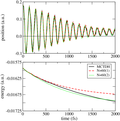
Figure 1: The energy relaxation (lower panel) and damped oscillations of the average position (upper panel) of the Morse oscillator in the weak coupling limit ($\gamma^{-1}=1630$ fs). The bath is assumed to be Ohmic with cutoff frequency $\omega_{\mathrm{c}}=2.9\cdot 10^{-3}$ a.u. and consists of $N=60$ TLS. The initial state was chosen to be a Gaussian displaced by $R_{0}=2\tilde{R}$ with a width of $\sigma=\tilde{R}$, where $\tilde{R}\approx 0.09129$. Thick solid lines refer to MCTDH calculations with a bath of harmonic oscillators (adopted from Ref. Nest and Meyer (2003)). Dashed lines refer to Surrogate Hamiltonian calculations with only single excitations. Thin lines refer to two simultaneous excitations allowed.

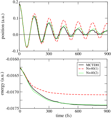
Figure 2: The energy relaxation (lower panel) and damped oscillations of the average position (upper panel) of the Morse oscillator in the intermediate coupling regime ($\gamma^{-1}=163$ fs). The bath parameters and the initial state are the same as in the weak coupling calculations. The number of bath modes is $N=40$. Thick solid lines refer to MCTDH calculations with a bath of harmonic oscillators (adopted from Ref. Nest and Meyer (2003)). Dashed lines refer to Surrogate Hamiltonian calculations with single excitations only. Thin lines refer to calculations with two allowed simultaneous excitations.

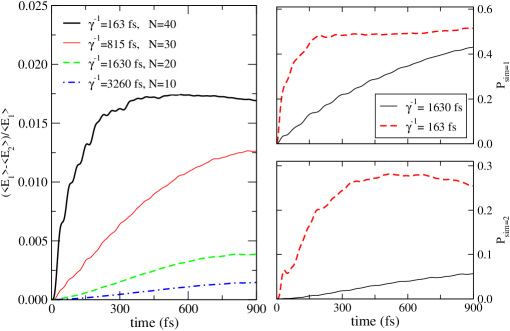
Figure 3: (Left panel) The relative difference in the effective subsystem energy ($\langle H_{\mathrm{S}}\rangle\ +0.5\langle H_{\mathrm{SB}}\rangle$) between the bath with only single excitations allowed $\langle E_{1}\rangle$ and the bath with two simultaneous excitations $\langle E_{2}\rangle$ as a function of time. The difference is calculated for a few coupling strengths. The simulation time is $t=900$ fs and the number of bath modes is $N=10\ldots 40$. (Right panel) The population $P_{\mathrm{sim}}$ of 1 and 2 simultaneous bath excitations is compared to the bath with two simultaneous excitations. The solid lines refer to the weak coupling limit ($\gamma^{-1}=1630$ fs) and the dashed lines refer to medium coupling ($\gamma^{-1}=163$ fs).

First a restricted Surrogate Hamiltonian is applied, which limits the possible system-bath correlations. The most extreme restriction includes only single excitations. The results for the weak coupling case ($\gamma^{-1}=1630$ fs) are shown in Fig. 1. For a short period of time the energy relaxes with the same rate in the two types of bath. However, after $t_{\mathrm{s}}\approx 500$ fs the rate decreases and eventually the system energy becomes constant. It should be pointed out, that the saturation time is not the recurrence (Poincaré) time ($t_{\mathrm{s}}<\tau_{\mathrm{rec}}$). This is confirmed by the fact that for time $t>t_{\mathrm{s}}$ the overall energy transfer from the bath back to the system is not complete. Calculating the population of the bath modes shows that at $t>t_{\mathrm{s}}$ most of the system energy is transferred to very few (or even one) bath modes, which are in resonance with the system’s frequency. Modes which are near to the resonance mode or modes become saturated and start to transfer the excitation back to the system. A dynamic “steady state” between the system and the bath is formed, where most of the modes transfer energy back, while one (or very few) continue to absorb energy from the system.

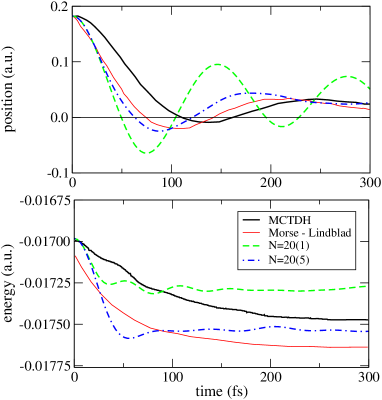
Figure 4: The energy relaxation (lower panel) and damped oscillations of the average position (upper panel) of the Morse oscillator in the strong coupling strength ($\gamma^{-1}=54$ fs). The bath parameters and the initial state are the same as in the weak coupling calculations. The number of bath modes is $N=20$. Solid lines refer to Nest and Meyer’s MCTDH calculations (adopted from Ref. Nest and Meyer (2003)), where the thick lines are the full-dimensional wave packet result and the thin lines refer to the Morse-Lindblad model. Dashed lines refer to Surrogate Hamiltonian calculations with single excitations. Dashed-dotted lines refer to a bath with five excitations allowed simultaneously.

When the number of simultaneous excitations is increased to two, the effect of saturation appears at a later stage ($t_{\mathrm{s}}>2000$ fs). The results become similar to those of Ref. Nest and Meyer (2003) and the values of the average position (see Fig. 1 (upper panel)) are nearly indistinguishable. We conclude that for the weak coupling case, the bath that has two simultaneous excitations is completely sufficient to reproduce the dynamics generated by all simultaneous excitations for times up to 2 ps.

The relaxation dynamics for medium coupling are shown in Fig. 2. A saturation effect was obtained for the bath restricted to single excitations. However, two simultaneous excitations were sufficient to overcome this saturation and converge the whole dynamics of the problem. A slight difference in the energy relaxation rate of the two baths is identified. The TLS bath causes stronger relaxation, but the results are still in good agreement with those of Ref. Nest and Meyer (2003). Since the initial state is a function of ${\bm{\mathrm{\hat{R}}}}$ and the system-bath coupling depends on ${\bm{\mathrm{\hat{R}}}}$ as well, the initial excitation influences the effective strength of the coupling. If the initial displacement, i.e. the initial excitation of the primary system, is decreased, the saturation is postponed. We can then deduce that the relaxation rate converges to the value of Ref. Nest and Meyer (2003). Combining the results of Figs. 1 and 2 leads to the conclusion that the differences between the two types of bath in the weak and intermediate coupling regimes are caused by the saturation of a few “central” modes in the spin bath. This saturation is postponed if the bath includes more correlations. For very weak coupling, these higher order system-bath correlations become insignificant.

The problem of including all system-bath correlations is therefore crucial in the medium and strong coupling regime. Fig. 3 shows the difference in the system energy ($\langle{\bm{\mathrm{\hat{H}}}}_{\mathrm{S}}\rangle\ +0.5\langle{\bm{\mathrm{\hat{H}}}}_{\mathrm{SB}}\rangle$) for two cases: a bath with only single excitations and a bath in which two simultaneous excitations are allowed. The calculations were made for different coupling strengths. As the coupling strength is reduced, the difference decreases. Thus in a very weak coupling limit, the TLS bath with only single excitations (no system-bath correlations) becomes sufficient to describe the dynamics for relatively long times. In this limit the TLS bath coincides completely with the harmonic bath.

The issue of including system-bath correlations has also been addressed in the MCTDH calculations. In Ref. Burghardt et al. (2003) the same system has been studied with the G-MCTDH method (the MCTDH with Gaussian expansion functions). Differences between the single-configurational (the Hartree limit) and the multi-configurational descriptions (with an increasing number of single particle functions) have been obtained for the energy relaxation process. In these calculations at least four single particle functions per resonant bath modes and two spf for secondary modes were required to achieve convergence in the relatively weak coupling limit ($\gamma^{-1}=500$ fs).

In the strong coupling regime (Fig. 4) there is considerable deviation between the two models. In the Surrogate Hamiltonian model the energy relaxes faster and the oscillator is damped after a single period. The relaxation rate obtained for the TLS bath is closer to the one obtained by the Morse-Lindblad model (adapted from Ref. Nest and Meyer (2003)). As expected convergence requires many simultaneous excitations. For example, a bath consisting of $N=20$ modes required at least five simultaneous excitations for converging the energy relaxation dynamics.

IV.2 The interaction between the bath modes.

The saturation of the TLS bath modes can be eliminated by allowing energy exchange between bath modes. This is done by adding to the bath Hamiltonian ${\bm{\mathrm{\hat{H}}}}_{\mathrm{B}}$ of Eq.(1) the term:

$${\bm{\mathrm{\hat{H}}}}_{\mathrm{int}}=\sum_{ij}\kappa_{ij}({\bm{\mathrm{\hat{\sigma}}}}_{i}^{\dagger}{\bm{\mathrm{\hat{\sigma}}}}_{j}+{\bm{\mathrm{\hat{\sigma}}}}_{j}^{\dagger}{\bm{\mathrm{\hat{\sigma}}}}_{i})\;,$$ (17)

where the parameter $\kappa_{ij}(=\kappa^{*}_{ji})$ is the interaction strength between two bath modes. The interaction can be restricted to the nearest neighbors in energy by the condition $\kappa_{ij}=0$ for $|i-j|>1$. The detailed algorithm of applying Eq.(17) in the bit representation has been described in Ref. Koch et al. (2002) in the context of pure dephasing.

The term ${\bm{\mathrm{\hat{\sigma}}}}_{i}^{\dagger}{\bm{\mathrm{\hat{\sigma}}}}_{j}+{\bm{\mathrm{\hat{\sigma}}}}_{j}^{\dagger}{\bm{\mathrm{\hat{\sigma}}}}_{i}$ describes a two quasi-particle interaction within the bath. A qualitative picture is based on an almost elastic exchange of energy between the two nearest neighbor bath modes which are almost degenerate. The process is described by a creation of an excitation in one mode at the expense of another and vice versa.

The new bath Hamiltonian including the interactions can be diagonalized leading to:

$${\bm{\mathrm{\hat{\tilde{H}}}}}_{\mathrm{B}}=\sum_{i}\tilde{\omega}_{i}{\bm{\mathrm{\hat{\tilde{\sigma}}}}}_{i}^{\dagger}{\bm{\mathrm{\hat{\tilde{\sigma}}}}}_{i}\;,$$ (18)

where $\tilde{\omega}_{i}$ are the eigenvalues of ${\bm{\mathrm{\hat{D}}}}^{\dagger}({\bm{\mathrm{\hat{H}}}}_{\mathrm{B}}+{\bm{\mathrm{\hat{H}}}}_{\mathrm{int}}){\bm{\mathrm{\hat{D}}}}$. In the new basis of $\{{\bm{\mathrm{\hat{\tilde{\sigma}}}}}_{i}\}$ the system-bath interaction term in Eq. (6) is also modified. However for sufficiently small $\kappa$ the eigenvalues of the bath change only slightly, but the saturation effect is postponed to a much later time.

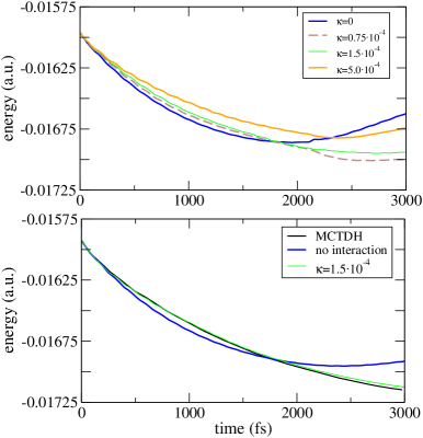
Figure 5: The energy relaxation with interaction between the bath modes is shown in the weak coupling limit ($\gamma^{-1}=1630$ fs). The bath is assumed to be Ohmic with cutoff frequency $\omega_{\mathrm{c}}=2.9\cdot 10^{-3}$ a.u. (Upper panel) The influence of the parameter $\kappa$ is shown for a bath of $N=40$ modes. (Lower panel) The energy relaxation is shown with the optimal parameter of $\kappa=1.5\cdot 10^{-4}$ (thin line). The thick solid line refers to MCTDH calculations with a bath of harmonic oscillators (Nest and Meyer (2003)). The dashed line refers to Surrogate Hamiltonian calculations with two simultaneous excitations allowed without interaction between the bath modes. The bath consists of $N=60$ modes.

Fig. 5 shows the influence of the interaction between the bath modes on energy relaxation in the weak coupling limit ($\gamma^{-1}=1630$ fs). The dynamics are calculated for a relatively long period of 3 ps. For such a long time the saturation effect is observed even for a bath with two simultaneous excitations. Since the saturation time $t_{\mathrm{s}}$ is determined mostly by the saturation of the few modes close to resonance with the subsystem, increasing the number of modes cannot prolong $t_{\mathrm{s}}$.

Adding an interaction between the bath modes leads to slower decay and delayed saturation (Cf Fig. 5, upper panel). This can be understood from the following considerations: the interaction term, Eq.(17), describes the transport of excitation from one bath mode to its nearest neighbor. Consequently, $\kappa$ determines how quickly the excitation is transported away from a TLS mode close to resonance with the primary system. On the other hand, the interaction energy, i.e. the expectation value of $\langle{\bm{\mathrm{\hat{H}}}}_{\mathrm{SB}}\rangle$, depends on the population of the primary system and of the bath modes close to it. If the population is removed from those bath modes and “diffuses” all over the bath, the interaction energy decreases and the decay becomes slower. This explains the upper panel of Fig. 5 which shows the energy relaxation for different values of $\kappa$.

An optimal value of $\kappa$ can minimize the differences between the spin and the harmonic bath. To demonstrate the effect, the calculations were carried out for $N=60$ bath modes and $\kappa=1.5\cdot 10^{-4}$ (Cf. the lower panel of Fig.  5). For this value of $\kappa$ the spectrum of the bath was only slightly altered (less than 1$\%$). The energy relaxation in this case is almost indistinguishable from the results obtained in Ref. Nest and Meyer (2003).

IV.3 Correlated versus uncorrelated states.

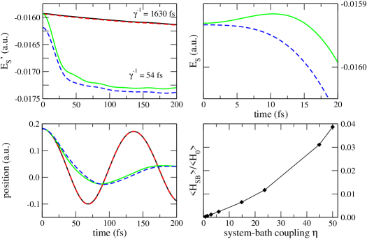
Figure 6: Effect of initial correlations. The energy relaxation and damped oscillations of the average position are shown for the initially uncorrelated (solid lines) and correlated (dashed lines) states. The dynamics for weak ($\gamma^{-1}=1630$ fs) and strong couplings ($\gamma^{-1}=54$ fs) are compared. A bath consisting of $N=10$ modes with 2 and 5 simultaneous excitations (for the weak and strong coupling, respectively) is sufficient to obtain the converged results. (Left) The effective subsystem energy (upper panel) ($E_{\mathrm{S}}^{{}^{\prime}}=\langle H_{\mathrm{S}}\rangle\ +0.5\langle H_{\mathrm{SB}}\rangle$) and the expectation value for the Morse coordinate (lower panel) are shown. (Right) The bare subsystem energy (upper panel) $E_{\mathrm{S}}=\langle H_{\mathrm{S}}\rangle$ in the strong coupling regime ($\gamma^{-1}=54$ fs) is shown for the short time dynamics. The energy stored in the system-bath coupling (lower panel) is calculated as a function of the coupling constant $\eta=M\gamma$.

The widely used assumption of an initially uncorrelated system-bath state is not consistent with most experimental situations Pechukas (1994); Romero-Rochin and Oppenheim (1989); Geva et al. (2000). The influence of initial correlations has been addressed in the context of the weak coupling approximation, where it appears as an additional inhomogeneous term Geva et al. (2000).

A fully correlated initial state is easily obtained in the Surrogate Hamiltonian method. Once the system-bath Hamiltonian ${\bm{\mathrm{\hat{H}}}}$ is set, the correlated ground state can be determined by propagating an initial guess wave function in imaginary time using ${\bm{\mathrm{\hat{H}}}}$ Kosloff and Tal-Ezer (1986b).

The influence of initial correlations is shown in Fig. 6. The uncorrelated state is identical to that of the previous calculations: the primary system is defined as a shifted Gaussian wave packet, while the bath is not excited. For the correlated initial state, the ground state of the total system was calculated first. Then this ground state was displaced by the shift operator in momentum space ${\bm{\mathrm{\hat{D}}}}=e^{-iR_{0}{\bm{\mathrm{\hat{k}}}}}$ with $R_{0}=2\tilde{R}$. The dynamics of the correlated state are compared to that of the uncorrelated state for weak and strong couplings ($\gamma^{-1}=1630$ fs and $\gamma^{-1}=54$ fs). The dashed and solid lines in Fig. 6 correspond to the initial state being correlated and uncorrelated, respectively.

The short-time dynamics differ for the correlated and uncorrelated cases, since the correlations need to be built up in the uncorrelated case Suárez et al. (1992). In the latter case an initial slippage in the system energy can be observed before the reduced dynamics appear to be Markovian (right upper panel). This effect is insignificant for weak coupling. Even for strong coupling, the differences between the correlated and uncorrelated cases were found to be very small. Apparently, the displacement is a stronger ”perturbation” than that caused by the correlations, i.e. the displacement establishes a new initial state Mančal and May (2001).

IV.4 Decoherence.

Decoherence has become a popular term used to describe loss of phase in coherent superpositions of quantum states due to interaction with a bath. It is therefore natural to compare the decoherence properties of the spin bath to those of the harmonic bath. The first difficulty is that there are different approaches to the definition of decoherence. Alicki Alicki (2002) identifies pure decoherence (dephasing) with the decay of the off-diagonal elements of the density operator, which is not accompanied by dissipation. He then argues that dephasing cannot be caused by a harmonic oscillator bath with a coupling, which is linear in coordinates or momenta.

Energy relaxation is also accompanied by loss of phase. For comparison, we will consider decoherence as a process caused by energy relaxation, which is characterized by a time $T_{1}=\gamma^{-1}$. The decoherence effect will be illustrated in terms of the dissipative dynamics of cat states, defined as a superposition of two coherent states. The interaction with the environment leads to decay of the coherences of such a superposition on an extremely short time scale, usually much shorter than the corresponding relaxation time scale Guilini et al. (1996). This process has been modeled using G-MCTDH by Burghardt et al. (2003), and as a result can be used for a comparative study.

The Wigner function of the cat state consists of two Gaussians centered at $(\pm R_{0},p_{0})$ and an interference term, which is centered at the origin. The off-diagonal part of the density matrix in the coherent-state basis, which contains information about quantum interferences between the two components of the cat state, decays with the rate $\gamma_{\mathrm{coh}}$. In the Markovian limit the decay rate is proportional to the square of the distance between the coherent states. For zero temperature it is given by Haake and Reibold (1985); Rajagopal (1998):

$$\gamma_{\mathrm{coh}}=\frac{\gamma M\omega_{0}\delta^{2}}{2\hbar}\;.$$ (19)

$\omega_{0}$ and $\delta$ are parameters of the primary system ($\omega_{0}$ represents the frequency of the harmonic oscillator, and $\delta$ is the separation distance between the coherent states).

The decoherence rate for a primary system coupled to a TLS bath is calculated and compared to the calculations for a bath of harmonic oscillators with the G-MCTDH method Burghardt et al. (2003). The calculations are performed for a cat state in a harmonic oscillator potential with $\omega_{0}=10^{-3}$ a.u. and $M=10^{5}$ a.u. The bath has the same parameters as for the previous calculations with damping rates of $\gamma^{-1}=1630$ fs and $\gamma^{-1}=500$ fs.

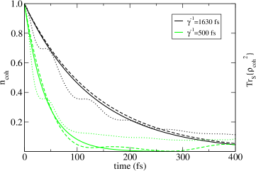
Figure 7: The decoherence effect in terms of decay of the coherence norm and off-diagonal elements in the energy representation. The coherence norm $n_{\mathrm{coh}}$ is shown as a function of time for two different couplings, $\gamma^{-1}=1630$ fs and $\gamma^{-1}=500$ fs. In the golden rule limit, off-diagonal elements of the reduced system density matrix $\rho(R,R^{{}^{\prime}})$ decay exponentially with the decoherence rates $\gamma_{\mathrm{coh}}^{-1}=130$ fs and $\gamma_{\mathrm{coh}}^{-1}=40$ fs (for the two given couplings, respectively). This decay is shown by the full lines. The dashed lines refer to the calculated decay of the decoherence norm. The dotted lines show the decay of ${\mathrm{tr}}_{S}\{{\bm{\mathrm{\hat{\rho}}}}_{\mathrm{coh}}^{2}\}$ in the energy representation.

A quantitative measure of decoherence of the primary system is the coherence norm used by Strunz et al. Strunz et al. (2003):

$$n_{\mathrm{coh}}(t)={\mathrm{tr}}_{S}\left\{{\bm{\mathrm{\hat{\rho}}}}_{\mathrm{S}}^{\mathrm{coh}}(t){\bm{\mathrm{\hat{\rho}}}}_{\mathrm{S}}^{\mathrm{coh\dagger}}(t)\right\}\;,$$ (20)

where ${\bm{\mathrm{\hat{\rho}}}}_{\mathrm{S}}^{\mathrm{coh}}$ refers to off-diagonal elements of the subsystem reduced density matrix in the basis of coherent states.

Since decoherence is a basis-dependent phenomenon, one can ask if it can also be measured in the basis of the eigenstates of the system Hamiltonian ${\bm{\mathrm{\hat{H}}}}_{\mathrm{S}}$. The question arises, whether these eigenstates form a pointer basis Paz and Zurek (1999) - the basis with respect to which off-diagonal elements in the reduced density operator disappear due to decoherence. To perform this test the system density operator ${\bm{\mathrm{\hat{\rho}}}}_{\mathrm{S}}(t)={\mathrm{tr}}_{B}\{{{\bm{\mathrm{\hat{\rho}}}}}\}$, which has been calculated in the coordinate basis is transformed to the basis of the ${\bm{\mathrm{\hat{H}}}}_{\mathrm{S}}$ eigenstates. Decomposing such a state to a dynamical and a static part leads to Banin et al. (1994):

$${\bm{\mathrm{\hat{\rho}}}}_{\mathrm{S}}(t)={\bm{\mathrm{\hat{\rho}}}}_{\mathrm{coh}}(t)+C^{2}{\bm{\mathrm{\hat{\rho}}}}_{\mathrm{S}}^{\mathrm{eq}}$$ (21)

where ${\bm{\mathrm{\hat{\rho}}}}_{\mathrm{S}}^{\mathrm{eq}}$ is the equilibrium stationary system density operator and $C^{2}$ is an overlap functional given by

$$C^{2}={\mathrm{tr}}_{S}\{{\bm{\mathrm{\hat{\rho}}}}_{\mathrm{S}}(t)\cdot{\bm{\mathrm{\hat{\rho}}}}_{\mathrm{S}}^{\mathrm{eq}}\}/{\mathrm{tr}}_{S}\{{{\bm{\mathrm{\hat{\rho}}}}_{\mathrm{S}}^{\mathrm{eq}}}^{2}\}~{}~{}.$$ (22)

${\bm{\mathrm{\hat{\rho}}}}_{\mathrm{coh}}(t)$ in Eq.(21), has no diagonal elements in the energy representation and is therefore traceless. Thus the decoherence effect is measured by the decay of ${\mathrm{tr}}_{S}\{{\bm{\mathrm{\hat{\rho}}}}_{\mathrm{coh}}^{2}\}$.
Fig. 7 shows the decay of the coherence norm $n_{\mathrm{coh}}$ and ${\mathrm{tr}}_{S}\{{\bm{\mathrm{\hat{\rho}}}}_{\mathrm{coh}}^{2}\}$ for two different coupling strengths (both are weak). The thick lines refer to a simple exponential decay predicted by Eq.(19) for a harmonic bath and confirmed by Ref. Burghardt et al. (2003). The dashed lines refer to the calculated decay of $n_{\mathrm{coh}}$, which is in good agreement with the prediction. The decay of ${\mathrm{tr}}_{S}\{{\bm{\mathrm{\hat{\rho}}}}_{\mathrm{coh}}^{2}\}$ (the dotted lines) has almost the same rate at a relatively short time. However, the off-diagonal elements of ${\bm{\mathrm{\hat{\rho}}}}_{\mathrm{S}}$ in the energy representation do not decay strictly to zero. Therefore, in this case, the system energy eigenstates cannot be considered as a pointer basis Paz and Zurek (1999).

IV.5 Entanglement.

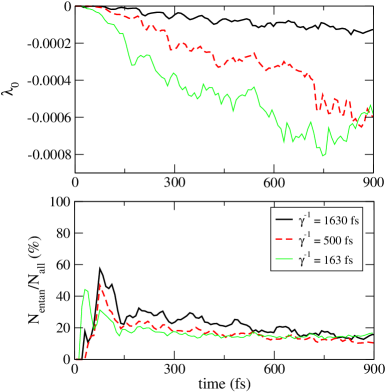
Figure 8: Measurement of entanglement between the bath modes as a function of time. (Upper panel) The smallest eigenvalue of the partial transposition $\rho^{\mathrm{T_{\mathrm{j}}}}$ of the reduced density matrix for pair of the bath modes ($i,j$) is calculated according to Appendix B. The negative eigenvalues are averaged over all possible combinations of the bath modes. (Lower panel) The relative number of entangled pairs of the bath modes as a function of time. The calculations are performed for three different system-bath coupling strengths ($\gamma^{-1}=1630,500,163$ fs). The bath consisting of $N=40$ modes with two simultaneous excitations allowed is used in all calculations.

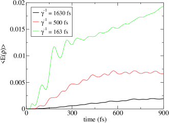
Figure 9: The entanglement of formation $E(\rho)$ is calculated for a couple of the bath modes ($i,j$). The average over all possible pairs is shown as a function of time. The calculations are performed for three different system-bath coupling strengths ($\gamma^{-1}=1630,500,163$ fs). The bath consisting of $N=40$ modes with two simultaneous excitations allowed is used in all calculations.

Entanglement between two quantum states is a manifestation of additional quantum correlation. For example entanglement between the system and the bath means ${\bm{\mathrm{\hat{\rho}}}}\neq{\bm{\mathrm{\hat{\rho}}}}_{\mathrm{S}}\otimes{\bm{\mathrm{\hat{\rho}}}}_{\mathrm{B}}$. In a dissipative environment it is expected that initial entanglement between parts of the system are lost leading to decoherence Zurek (1982); Joos and Zeh (1985). In addition a bath can also provide an indirect interaction between totally decoupled parts of the primary system and entangle them Braun (2002); Benatti et al. (2003).

The difference between the harmonic and the spin baths should be manifested in another type of entanglement - quantum correlations between different bath modes. A system interacting with the spin bath, can induce entanglement between two spin modes, which are not directly interacting with each other. In the harmonic bath on the other hand, a system linearly coupled to different modes is not able to entangle those modes (see Appendix A).

Peres A.Peres (1996) and Horodecki et al. Horodecki et al. (1996) have provided a criterion, based on partial transposition, to determine whether a given mixed state of two subsystems is entangled (cf Appendix B). Since the criterion is defined only for two coupled TLS, the study of entanglement is limited to two bath modes (i) and (j). The density operator of any two bath modes ${\bm{\mathrm{\hat{\rho}}}}_{\mathrm{ij}}$ is obtained as a partial trace of ${\mathrm{tr}}_{\mathrm{k\neq i,j}}\{{\bm{\mathrm{\hat{\rho}}}}_{\mathrm{B}}\}$ over the rest of the bath modes, where the density operator of the bath is ${\bm{\mathrm{\hat{\rho}}}}_{\mathrm{B}}={\mathrm{tr}}_{S}\{{\bm{\mathrm{\hat{\rho}}}}\}$. The procedure checks whether the partial transposition of ${\bm{\mathrm{\hat{\rho}}}}_{\mathrm{ij}}$ with respect to one of the modes has negative eigenvalues. The smallest eigenvalue $\lambda_{0}$ of the partial transpose matrix $\rho^{\mathrm{T_{\mathrm{j}}}}$ constitutes the criteria. Then the eigenvalues with $\lambda_{0}<0$ are averaged over all entangled pairs of bath modes.

In Fig. 8 the averaged parameter $\lambda_{0}$ is shown as a function of time for three different coupling strengths. The entanglement calculations were based on converged results obtained for a bath of $N=40$ modes. This was sufficient to a time scale of 900 fs, for all three system bath coupling strength considered. Since at $t=0$ the bath is not excited, there are no entangled bath modes, therefore $\lambda_{0}=0$ for all pairs. As $t$ increases $\lambda_{0}$ becomes negative for some of the pairs of the bath modes, meaning that these modes become entangled. As time progresses, the number of entangled pairs saturates for all three couplings (Cf Fig. 8, lower panel). Therefore, the increase in the absolute value of $\lambda_{0}$ is related primarily to the growth in population of the entangled modes. The maximum in the number of entangled modes for an early time may be associated with the creation of higher-order entanglement terms where three or more simultaneous excitations become important. Such higher-order entanglement is not captured by the Peres-Horodecki parameter.

To characterize the degree of entanglement we use an additional measure, the entanglement of formation introduced by Wootters et al. Bennett et al. (1996); Hill and Wootters (1997); Wootters (1998) (Cf. Appendix B). For any $2\otimes 2$ mixed state this quantity varies from zero (separable states) to one (maximally entangled states). Our results (Cf. Fig. 9) are obtained by averaging the entanglement of formation $E(\rho_{\mathrm{ij}})$ (for two bath modes $i$ and $j$) over all possible pairs of modes. The dynamics of $\langle E(\rho)\rangle$ is similar to those of the partial transpose parameter. It should be noted that the growth of entanglement shown in Figs. 8-9 is exclusive to the spin bath.

V Summary and Conclusions

The similarities and differences of the relaxation dynamics of a primary system coupled to a spin or to a harmonic bath have been analyzed. The study was facilitated by the ability to obtain converged numerical results for finite period in time. In both cases this task becomes possible by employing a large but finite number of bath modes and controlling the degree of correlation.

V.1 The similarities

For all cases studied the extremely short time dynamics was identical. This period represents the inertial response of the bath and is characterized by a zero derivative of the energy at the initial time $t=0$. This non-Markovian dynamical evolution, ”the slippage”, is quite short and in many cases it can be ignored. The initial dynamics is closely related to the issue of the choice of the initial state. Preferably it should represent equilibrium system bath correlation and not be a product state. The Surrogate Hamiltonian method allows to create such a fully correlated initial state of the system-bath entity. However, in the present model differences in the dynamics between correlated and uncorrelated states seem to be insignificant, even in the strong coupling case. It is expected that the same phenomena would be observed in the harmonic bath.

For weak system-bath coupling the dynamics induced by both baths are also similar. This is a numerical confirmation that in the weak coupling limit the harmonic bath can be mapped to the spin bath Caldeira et al. (1993); Forsythe and Makri (1998); Tsonchev and Pechukas (1999). In addition in this limit the spin bath converges with only single excitations of the bath modes meaning that the system and bath are almost disentangled. This fact is consistent with the convergence to the Markovian limit Lindblad (1998).

The decoherence properties of the harmonic and spin baths as determined by the loss of phase of cat states are found to be quite similar. This result is somewhat surprising since the ergodic properties of the two baths are different. To rationalize, one should notice that the coherence in cat states composed of a superposition of two coherent states in a single mode does not represent entanglement. Therefore, this phase loss does not characterize decoherence in accordance with Alicki’s notion Alicki (2002). Moreover when a pure dephasing term was added it was found that it did not erode the phase coherence between cat states Vala and Kosloff (2002). We conclude that the decoherence properties of the two baths still require a further study.

V.2 The differences

The spin and harmonic baths begin to deviate when the initial excitation of the primary system is increased. This difference is observed for excitations where the dynamics generated by the harmonic bath is still Markovian. The first indication of differences is the necessity of two simultaneous bath excitation to converge the spin bath. For larger time periods, the spin bath saturates limiting the ability to assimilate the system’s energy. The conclusion is that the limit of weak coupling is more restrictive in the spin bath case. The effect of saturation can be reduced if the bath Hamiltonian includes a mode-mode coupling term. This term causes diffusion of excitation between the modes, spreading the excitation over a greater number of bath modes. Thus bath modes, which are relatively far from resonance with the primary system become populated and the saturation is suppressed. Practically, this allows to increase the convergence timescale of the spin bath.

In the medium coupling regime there is an overall good agreement between the two models. The spin bath, however, causes stronger relaxation, a fact, which becomes even more visible in the case of strong coupling. In this regime the deviations between the two baths become significant.

The possibility of entanglement of bath modes mediated by the primary system is a major conceptual difference between the spin and harmonic baths. In the spin bath after a short initial period where only single excitations are excited, entanglement between pairs of spin sets in with what seems as an exponential growth. At later times the pair entanglement is replaced by higher order terms and the pair entanglement saturates. All these correlations are absent from the harmonic bath nevertheless the dynamics of the the primary systems are not very different except for extremely strong coupling. It could be possible that the in the present model the primary system and the system bath coupling terms are oversimplified. In addition the simulations should be extended to finite temperatures, where different behavior of harmonic and spin baths is expected except for the weak coupling regime Tsonchev and Pechukas (1999); Caldeira et al. (1993); Golosov et al. (1999). The recently proposed random phase method Gelman and Kosloff (2003) may be used to extend the above models to finite temperature applications.

The present study is an important step in establishing the Surrogate Hamiltonian method as a practical simulation tool. The elucidation of the system-bath dynamics allows to tailor a simulation package in particular for ultrafast dynamical processes.

Appendix A Harmonic bath vs spin bath.

The differences between harmonic and spin baths can be illuminated by studying the simple system of a spin-$\frac{1}{2}$ coupled to a bath. For the harmonic bath the total Hamiltonian in second quantization is given by:

$${\bm{\mathrm{\hat{H}}}}=\frac{1}{2}\Omega\hat{\sigma}_{z}+\sum_{j}\omega_{j}{\bm{\mathrm{\hat{b}}}}_{j}^{{\dagger}}{\bm{\mathrm{\hat{b}}}}_{j}+\sum_{j}\lambda_{j}({\bm{\mathrm{\hat{b}}}}_{j}+{\bm{\mathrm{\hat{b}}}}_{j}^{{\dagger}})(\hat{\sigma}_{+}+\hat{\sigma}_{-})\;.$$ (23)

Thus the Heisenberg equations of motion for the system operators are:

$$\frac{d}{dt}\hat{\sigma}_{\pm}=\frac{1}{i}[\hat{\sigma}_{\pm},{\bm{\mathrm{\hat{H}}}}]=\pm i\Omega\hat{\sigma}_{\pm}-i\hat{\sigma}_{z}\sum_{j}\lambda_{j}({\bm{\mathrm{\hat{b}}}}_{j}+{\bm{\mathrm{\hat{b}}}}_{j}^{{\dagger}})\;.$$ (24)

Similarly, the equations of motion for the bath operators are:

$$\frac{d}{dt}{\bm{\mathrm{\hat{b}}}}_{j}=-i\omega_{j}{\bm{\mathrm{\hat{b}}}}_{j}-i\lambda_{j}(\hat{\sigma}_{+}+\hat{\sigma}_{-})\;.$$ (25)

Since the annihilation and creation operators ${\bm{\mathrm{\hat{b}}}}_{j}$ and ${\bm{\mathrm{\hat{b}}}}_{j}^{{\dagger}}$, satisfy the standard Bose commutation relation, $[{\bm{\mathrm{\hat{b}}}}_{j},{\bm{\mathrm{\hat{b}}}}_{j^{\prime}}^{{\dagger}}]=\delta_{j,j^{\prime}}$, a closed set of equations is obtained for each of the independent bath modes.
Now, let us consider a different model, where the primary system is coupled to a bath of spins-$\frac{1}{2}$. The total Hamiltonian may be written in the form:

$${\bm{\mathrm{\hat{H}}}}=\Omega\hat{\sigma}_{z}^{0}+\frac{1}{2}\sum_{j}\omega_{j}{\bm{\mathrm{\hat{\sigma}}}}_{z}^{j}-\frac{1}{2}\sum_{j}\lambda_{j}\hat{\sigma}_{+}^{0}{\bm{\mathrm{\hat{\sigma}}}}_{-}^{j}+h.c.\;,$$ (26)

where ${\bm{\mathrm{\hat{\sigma}}}}_{x,y,z}$ designates the set of Pauli operators and ${\bm{\mathrm{\hat{\sigma}}}}_{\pm}^{i}={\bm{\mathrm{\hat{\sigma}}}}_{x}^{i}\pm{\bm{\mathrm{\hat{\sigma}}}}_{y}^{i}$ are the usual ladder operators. For simplicity, we consider a system (0) consisting of a spin-$\frac{1}{2}$ which interacts with a pair (1,2) of spins. Thus, the Hamiltonian of the whole system reads:

$${\bm{\mathrm{\hat{H}}}}=\Omega\hat{\sigma}_{z}^{0}+\frac{1}{2}(\omega_{1}{\bm{\mathrm{\hat{\sigma}}}}_{z}^{1}+\omega_{2}{\bm{\mathrm{\hat{\sigma}}}}_{z}^{2})-\frac{\lambda_{1}}{2}(\hat{\sigma}_{+}^{0}{\bm{\mathrm{\hat{\sigma}}}}_{-}^{1}+\hat{\sigma}_{-}^{0}{\bm{\mathrm{\hat{\sigma}}}}_{+}^{1})-\frac{\lambda_{2}}{2}(\hat{\sigma}_{+}^{0}{\bm{\mathrm{\hat{\sigma}}}}_{-}^{2}+\hat{\sigma}_{-}^{0}{\bm{\mathrm{\hat{\sigma}}}}_{+}^{2})\;.$$ (27)

The Heisenberg equations of motion for the system operator are:

$$\frac{d}{dt}\hat{\sigma}_{\pm}^{0}=\pm i(2\Omega\hat{\sigma}_{\pm}^{0}+\frac{\lambda_{1}}{2}\hat{\sigma}_{z}^{0}{\bm{\mathrm{\hat{\sigma}}}}_{\pm}^{1}+\frac{\lambda_{2}}{2}\hat{\sigma}_{z}^{0}{\bm{\mathrm{\hat{\sigma}}}}_{\pm}^{2})\;,$$ (28)

and the equation of motion for the bath operator reads:

$$\frac{d}{dt}{\bm{\mathrm{\hat{\sigma}}}}_{\pm}^{1,2}=\pm i(\omega_{1,2}{\bm{\mathrm{\hat{\sigma}}}}_{\pm}^{1,2}+\frac{\lambda_{1,2}}{2}\sigma_{\pm}^{0}{\bm{\mathrm{\hat{\sigma}}}}_{z}^{1,2})\;.$$ (29)

The commutation relations for spin operators are different from those of bosons:

$$[{\bm{\mathrm{\hat{\sigma}}}}_{i},{\bm{\mathrm{\hat{\sigma}}}}_{j}]=-2i{\bm{\mathrm{\hat{\sigma}}}}_{k}\;,$$ (30)

which makes the set of the equations above non-closed. After some algebra, the equation for the bath operators becomes:

$$\frac{d}{dt}(\hat{\sigma}_{z}^{0}{\bm{\mathrm{\hat{\sigma}}}}_{\pm}^{1,2})=\pm i\omega_{1,2}\hat{\sigma}_{z}^{0}{\bm{\mathrm{\hat{\sigma}}}}_{\pm}^{1,2}\pm i\frac{\lambda_{1}}{2}\hat{\sigma}_{\pm}^{0}+i\lambda_{2}(\hat{\sigma}_{+}^{0}{\bm{\mathrm{\hat{\sigma}}}}_{\pm}^{1,2}{\bm{\mathrm{\hat{\sigma}}}}_{-}^{2,1}-\hat{\sigma}_{-}^{0}{\bm{\mathrm{\hat{\sigma}}}}_{\pm}^{1,2}{\bm{\mathrm{\hat{\sigma}}}}_{+}^{2,1})\;.$$ (31)

The triple correlations of the type $\hat{\sigma}_{+}^{0}{\bm{\mathrm{\hat{\sigma}}}}_{\pm}^{1}{\bm{\mathrm{\hat{\sigma}}}}_{-}^{2}$ is a manifestation of the build-up of quantum entanglement - a specific correlation between different modes, which has no analogy in classical physics. These correlations make a difference between the spin bath and the harmonic oscillator one, since the latter does not have quantum correlations between the bath modes.

Appendix B Entanglement between different bath modes.

In order to check whether the reduced two-system density matrix ${\bm{\mathrm{\hat{\rho}}}}$ is entangled, first we will use the partial transposition criterion proposed by Peres A.Peres (1996) and Horodecki et al. Horodecki et al. (1996). A mixed state described by density matrix ${\bm{\mathrm{\hat{\rho}}}}$ is non-separable (and therefore cannot be written as a product state of two subsystems (i) and (j), ${\bm{\mathrm{\hat{\rho}}}}={\bm{\mathrm{\hat{\rho}}}}_{\mathrm{i}}\otimes{\bm{\mathrm{\hat{\rho}}}}_{\mathrm{j}}$), iff the partial transposition of ${\bm{\mathrm{\hat{\rho}}}}$ with respect to one of the two subsystems has negative eigenvalues. The partial transpose ${\bm{\mathrm{\hat{\rho}}}}^{\mathrm{T_{\mathrm{j}}}}$ is obtained by transposing in a matrix representation of ${\bm{\mathrm{\hat{\rho}}}}$ only those indices corresponding to subsystem (j), i.e. $\rho^{\mathrm{T_{\mathrm{j}}}}_{\mathrm{m\mu,n\nu}}=\rho_{\mathrm{m\nu,n\mu}}$. The following notation for matrix elements of a composite system is used:

$$\rho_{\mathrm{m\mu,n\nu}}=\left\langle e_{m}\otimes f_{\mu}|{\bm{\mathrm{\hat{\rho}}}}|e_{n}\otimes f_{\nu}\right\rangle\;,$$ (32)

where ${e_{m}}$ and ${f_{\mu}}$ denote the arbitrary orthonormal bases in Hilbert space describing the first (i) and second (j) system, respectively.
Checking the positivity of the partial transpose is equivalent to checking the signs of the eigenvalues of ${\bm{\mathrm{\hat{\rho}}}}^{\mathrm{T_{\mathrm{j}}}}$ or ,alternatively, the signs of the following determinants:

$$W_{1}=\rho^{\mathrm{T_{j}}}_{\mathrm{11,11}}\rho^{\mathrm{T_{j}}}_{\mathrm{22,22}}-\rho^{\mathrm{T_{j}}}_{\mathrm{11,22}}\rho^{\mathrm{T_{j}}}_{\mathrm{22,11}},\;\;W_{2}=\rho^{\mathrm{T_{j}}}_{\mathrm{12,12}}\rho^{\mathrm{T_{j}}}_{\mathrm{21,21}}-\rho^{\mathrm{T_{j}}}_{\mathrm{12,21}}\rho^{\mathrm{T_{j}}}_{\mathrm{21,12}}.$$ (33)

In the case when one of the above determinants is negative, the state ${\bm{\mathrm{\hat{\rho}}}}$ is non-separable, and hence there is entanglement between the two subsystems ${\bm{\mathrm{\hat{\rho}}}}_{\mathrm{i}}$, ${\bm{\mathrm{\hat{\rho}}}}_{\mathrm{j}}$.

Another entanglement measure for a mixed state of two spin-$\frac{1}{2}$ particles is the entanglement of formation Bennett et al. (1996); Hill and Wootters (1997); Wootters (1998). Explicitly, for the reduced two-system density matrix ${\bm{\mathrm{\hat{\rho}}}}$ the entanglement of formation is defined by

$$E(\rho)=h\left(\frac{1}{2}\left[1+\sqrt{1-\mathcal{C}(\rho)^{2}}\right]\right)\;,$$ (34)

where $h$ is the binary entropy function $h(x)=-x\log_{2}{x}-(1-x)\log_{2}(1-x)$ and $\mathcal{C}(\rho)$ is the concurrence. The concurrence is calculated in the following way: first we define the ”spin-flipped” density matrix to be

$$\widetilde{\rho}=(\sigma_{y}\otimes\sigma_{y})\rho^{*}(\sigma_{y}\otimes\sigma_{y})\;,$$ (35)

where the asterisk denotes complex conjugation of ${\bm{\mathrm{\hat{\rho}}}}$ in the standard basis $\left\{|00\rangle,|01\rangle,|10\rangle,|11\rangle,\right\}$ and $\sigma_{y}$ expressed in the same basis is the matrix

$$\sigma_{y}=\left({\begin{array}[]{cc}0&-i\\ i&0\end{array}}\right)\;.$$ (36)

As both $\rho$ and $\widetilde{\rho}$ are positive operators, it follows that the product $\rho\widetilde{\rho}$, though non-Hermitian, also has only real and non-negative eigenvalues. Let the square roots of these eigenvalues, in decreasing order , be $\lambda_{1}$, $\lambda_{2}$, $\lambda_{3}$, and $\lambda_{4}$. Then the concurrence of the density matrix $\rho$ is defined as $\mathcal{C}=\max\{\lambda_{1}-\lambda_{2}-\lambda_{3}-\lambda_{4},0\}$. It should be noted that $\mathcal{C}=0$ corresponds to an unentangled state, while $\mathcal{C}=1$ - to a completely entangled state and the entanglement of formation $E$ is a monotonically increasing function of $\mathcal{C}$.

References

- Weiss (1999) U. Weiss, Quantum Dissipative Systems (World Scientific, 1999).
- Feynman and Vernon (1963) R. Feynman and F. Vernon, Ann. Phys. 24, 118 (1963).
- Louisell (1990) W. H. Louisell, Quantum Statistical Properties of Radiation (Wiley, New York, 1990).
- Baer and Kosloff (1997) R. Baer and R. Kosloff, J. Chem. Phys. 106, 8862 (1997).
- Caldeira et al. (1993) A. O. Caldeira, A. H. C. Neto, and T. O. de Carvalho, Phys. Rev. B 48, 13974 (1993).
- Forsythe and Makri (1998) K. Forsythe and N. Makri, Phys. Rev. B 60, 972 (1998).
- Tsonchev and Pechukas (1999) S. Tsonchev and P. Pechukas, Phys. Rev. E 61, 6171 (1999).
- Prokof’ev and Stamp (2000) N. V. Prokof’ev and P. Stamp, Rep. Prog. Phys. 63, 669 (2000), and references therein.
- Shao and Hänggi (1998) J. Shao and P. Hänggi, Phys. Rev. Lett. 81, 5710 (1998).
- Bader and Berne (1994) J. S. Bader and B. J. Berne, J. Chem. Phys. p. 8359 (1994).
- Koch et al. (2003a) C. P. Koch, T. Klüner, H.-J. Freund, and R. Kosloff, J. Chem. Phys. 119, 1750 (2003a).
- Nest and Meyer (2003) M. Nest and H.-D. Meyer, J. Chem. Phys. 119, 24 (2003).
- Burghardt et al. (2003) I. Burghardt, M. Nest, and G. A. Worth, J. Chem. Phys. 119, 5364 (2003).
- Redfield (1955) A. G. Redfield, Phys. Rev. 98, 1787 (1955).
- Redfield (1957) A. G. Redfield, IBM Jr. 1, 19 (1957).
- Lindblad (1976) G. Lindblad, Commun. Math. Phys. 48, 119 (1976).
- Gorini et al. (1976) V. Gorini, A. Kossokowski, and E. C. G. Sudarshan, J. Math. Phys. 17, 821 (1976).
- Alicki and Lendi (1987) R. Alicki and K. Lendi, Quantum Dynamical Semigroups and Applications (Springer-Verlag, 1987).
- Makri (1999) N. Makri, J. Phys. Chem. B 103, 2823 (1999).
- van Kampen (1992) N. G. van Kampen, Stochastic Processes in Physics and Chemistry (North-Holland, Amsterdam, 1992).
- Koch et al. (2003b) C. P. Koch, T. Klüner, H.-J. Freund, and R. Kosloff, Phys. Rev. Lett. 90, 117601 (2003b).
- Meyer et al. (1993) H.-D. Meyer, U. Manthe, and L. S. Cederbaum, in Numerical Grid Methods and Their Application to Schrödinger equation (Kluwer Academic, The Netherlands, 1993), pp. 141–152.
- Worth et al. (1996) G. A. Worth, H.-D. Meyer, and L. S. Cederbaum, J. Chem. Phys. 105, 4412 (1996).
- Wang (2000) H. Wang, J. Chem. Phys. 113, 9948 (2000).
- Kosloff (1993) R. Kosloff, ”The Fourier Method”, in Numerical Grid Methods and Their Application to Schrödinger equation (Kluwer Academic, The Netherlands, 1993).
- Kosloff and Tal-Ezer (1986a) R. Kosloff and H. Tal-Ezer, Chem. Phys. Lett. 127, 223 (1986a).
- Koch et al. (2002) C. P. Koch, T. Klüner, and R. Kosloff, J. Chem. Phys. 116, 7983 (2002).
- Pechukas (1994) P. Pechukas, Phys. Rev. Lett. 73, 1060 (1994).
- Romero-Rochin and Oppenheim (1989) V. Romero-Rochin and I. Oppenheim, Physica A 155, 52 (1989).
- Geva et al. (2000) E. Geva, E. Rosenman, and D. Tannor, J. Chem. Phys. 113, 1380 (2000).
- Kosloff and Tal-Ezer (1986b) R. Kosloff and H. Tal-Ezer, Chem. Phys. Lett. 127, 223 (1986b).
- Suárez et al. (1992) A. Suárez, R. Silbey, and I. Oppenheim, J. Chem. Phys. 97, 5101 (1992).
- Mančal and May (2001) T. Mančal and V. May, J. Chem. Phys. 114, 1510 (2001).
- Alicki (2002) R. Alicki, arXiv:quant-ph 0205173 (2002).
- Guilini et al. (1996) D. Guilini, E. Joos, C. Kiefer, J. Kupsch, I.-O. Stamatescu, and H. D. Zeh, eds., Decoherence and the Appearence of a Classical World in Quantum Theory (Springer-Verlag, Berlin, 1996).
- Haake and Reibold (1985) F. Haake and R. Reibold, Phys. Rev. A 32, 2462 (1985).
- Rajagopal (1998) A. K. Rajagopal, Phys. Lett. A 246, 237 (1998).
- Strunz et al. (2003) W. T. Strunz, F. Haake, and D. Braun, Phys. Rev. A 67, 022101 (2003).
- Paz and Zurek (1999) J. P. Paz and W. H. Zurek, Phys. Rev. Lett. 82, 5181 (1999).
- Banin et al. (1994) U. Banin, A. Bartana, S. Ruhman, and R. Kosloff, J. Chem. Phys. 101, 8461 (1994).
- Zurek (1982) W. H. Zurek, Phys. Rev. D 26, 1862 (1982).
- Joos and Zeh (1985) E. Joos and H. D. Zeh, Z. Phys. B 59, 223 (1985).
- Braun (2002) D. Braun, Phys. Rev. Lett. 89, 277901 (2002).
- Benatti et al. (2003) F. Benatti, R. Floreanini, and M. Piani, Phys. Rev. Lett. 91, 070401 (2003).
- A.Peres (1996) A.Peres, Phys. Rev. Lett. 77, 1413 (1996).
- Horodecki et al. (1996) M. Horodecki, P. Horodecki, and R. Horodecki, Phys. Lett. A 223, 1 (1996).
- Bennett et al. (1996) C. H. Bennett, D. P. DiVincenzo, J. A. Smolin, and W. K. Wootters, Phys. Rev. A 54, 3824 (1996).
- Hill and Wootters (1997) S. Hill and W. K. Wootters, Phys. Rev. Lett. 78, 5022 (1997).
- Wootters (1998) W. K. Wootters, Phys. Rev. Lett. 80, 2245 (1998).
- Lindblad (1998) G. Lindblad, J. Math. Phys. 39, 2763 (1998).
- Vala and Kosloff (2002) J. Vala and R. Kosloff (2002), unpublished.
- Golosov et al. (1999) A. A. Golosov, S. I. Tsonchev, P. Pechukas, and R. A. Friesner, J. Chem. Phys. 111, 9918 (1999).
- Gelman and Kosloff (2003) D. Gelman and R. Kosloff, Chem. Phys. Lett. 381, 129 (2003).