Optimal Control of Quantum Dissipative Dynamics: Analytic solution for cooling the three level $\Lambda$ system

Abstract

We study the problem of optimal control of dissipative quantum dynamics. Although under most circumstances dissipation leads to an increase in entropy (or a decrease in purity) of the system, there is an important class of problems for which dissipation with external control can decrease the entropy (or increase the purity) of the system. An important example is laser cooling. In such systems, there is an interplay of the Hamiltonian part of the dynamics, which is controllable and the dissipative part of the dynamics, which is uncontrollable. The strategy is to control the Hamiltonian portion of the evolution in such a way that the dissipation causes the purity of the system to increase rather than decrease. The goal of this paper is to find the strategy that leads to maximal purity at the final time. Under the assumption that Hamiltonian control is complete and arbitrarily fast, we provide a general framework by which to calculate optimal cooling strategies. These assumptions lead to a great simplification, in which the control problem can be reformulated in terms of the spectrum of eigenvalues of $\rho$, rather than $\rho$ itself. By combining this formulation with the Hamilton-Jacobi-Bellman theorem we are able to obtain an equation for the globaly optimal cooling strategy in terms of the spectrum of the density matrix. For the three-level $\Lambda$ system, we provide a complete analytic solution for the optimal cooling strategy. For this system it is found that the optimal strategy does not exploit system coherences and is a ’greedy’ strategy, in which the purity is increased maximally at each instant.

I Introduction

In the last 15 years, optimal control theory (OCT) has been applied to an increasingly wide number of problems in physics and chemistry whose dynamics are governed by the time-dependent Schrödinger equation (TDSE). These problems include control of chemical reactions Tannor85 ; Tannor86 ; Tannor88 ; Kosloff89 ; Rice2000 ; Shapiro03 ; Brixner03 ; Mitric02 , state-to-state population transfer Peirce88 ; Shi91 ; Jakubetz90 ; Shen94 , shaped wavepackets Yan93 , NMR spin dynamics Khaneja01 , Bose-Einstein condensation Hornung ; Sklarz02.1 ; sklarz02.2 , quantum computing Rangan01 ; Tesch01 ; Palao02 , oriented rotational wavepackets Leibscher03 , etc. Rabitz ; Gordon97 . More recently, there has been vigorous effort in studying the control of systems governed by the Liouville-von Neumann (LVN) equation, where the central object is the density matrix, rather than the wavefunction Bartana93 ; Bartana ; TannorRot ; Cao97 ; Gross98 ; Ohtsuki03 ; Khaneja03 . The Liouville-von Neumann equation is an extension of the TDSE that allows for the inclusion of dissipative processes. Important examples of what may be thought of as quantum control processes that require the use of the LVN include laser control of chemical reactions in solution, laser cooling, and coherence transfer in multi-spin systems. In all these cases, the external field (the laser or the RF field) is the coherent control, while the source of dissipation is contact with the environment. In the case of laser cooling, the environment is the vacuum modes of the electromagnetic field and the source of dissipation is spontaneous emission.

In the majority of problems on control of quantum systems dissipation is a nuisance; the purpose of the control is to either avoid, delay or cancel the dissipation process. Yet there is a remarkable exception to this pattern — laser cooling. The goal of laser cooling is expressed alternatively as increasing the phase space density, or decreasing the entropy of the system. Purely Hamiltonian manipulations can in fact do neither, and therefore dissipation, rather than being a nuisance, is actually necessary to achieve true cooling. The optimal control of systems of this type is fascinating. The control itself, no matter what its time-dependence, leads only to Hamiltonian evolution and hence no true progress toward the objective. On the other hand, the dissipation, while it is capable of producing progress toward the objective, is fundamentally not controllable and could in fact lead to a decrease in the objective.

In ref. TannorRot , we elucidated the interplay of the controlled, Hamiltonian evolution, and the uncontrolled, dissipative evolution in producing cooling. The “cooling laser”, while not directly cooling the system, in fact steers it to a region of parameter space where spontaneous emission leads to cooling rather than heating. We define such a controlled manipulation as a ”purity increasing transformation”. We believe that the study of such transformations in their general mathematical context is of extreme interest, both in terms of discovering a wider class of physical processes where purity, and therefore coherence content can be increased, as well as because of the rich mathematical structure of the problems involving interplay of Hamiltonian and dissipative dynamics.

In TannorRot , we solved the problem of optimal cooling for a 2-level system completely, under the assumption of complete and rapid Hamiltonian control. We showed that the optimal cooling strategy in the 2-level system avoids producing coherences in the density matrix. Here we present a general framework for the analysis of optimal control in a system of $N$ excited states coupled radiatively to $M$ ground states, under the same assumptions. Using this framework we explicitly provide the optimal strategy for cooling of a three level $\Lambda$ system.

We first introduce the Lindblad dissipation model and a generalized concept of purity in section II. In Section II.3 the problem of optimal cooling of a quantum mechanical system is formulated. It is shown in Section III that this problem can be reformulated solely in terms of the eigenvalue distribution of the density operator. In doing this, we derive a reduced equation of motion for the spectral evolution under dissipation, parameterized by the unitary control (Sections III.2 and III.3). Section IV introduces the mathematical tools for finding optimal cooling strategies, namely the Hamilton-Jacobi-Bellman theorem. Section V provides an explicit description of the optimal cooling strategy for the three level $\Lambda$ system and proves its optimality. Finally we discuss future directions and conclude in Section VI.

II Setting up the control problem

II.1 The system equations of motion and the Lindblad formula for dissipation

Let $\rho$ denote the density matrix of an $N$ level quantum system (see figure 1). The density matrix evolves under the Liouville von Neumann (LVN) equation which takes the form

$$\dot{\rho}=-i[H(t),\rho]+L(\rho)$$ (1)

where $-i[H,\rho]$ is the unitary evolution of the quantum system and $L(\rho)$ is the dissipative part of the evolution. The term $L(\rho)$ is linear in $\rho$ and is given by the Lindblad form Lindblad ; Alicki86 , i.e.

$$L(\rho)=\sum_{ij}F_{ij}\rho F_{ij}^{\dagger}-\frac{1}{2}\{F_{ij}^{\dagger}F_{ij},\rho\},$$

where $F_{ij}$ are the Lindblad operators. In this manuscript, we assume the only relaxation mechanism is spontaneous emission and therefore we take $F_{ij}=\sqrt{\gamma_{ij}}E_{ij}$ where the operator $E_{ij}={|{i}\rangle}{\langle{j}|}$ and $\gamma_{ij}$ represents the rate of spontaneous emission from level $j$ to level $i$. Eq. (1) has the following three well known properties: 1) ${\rm Tr}(\rho)$ remains unity for all time, 2) $\rho$ remains a Hermitian matrix, and 3) $\rho$ stays positive semi-definite, i.e. that $\rho$ never develops non-negative eigenvalues.

The first property follows from

$${\rm Tr}(\dot{\rho})={\rm Tr}(-i[H,\rho])+{\rm Tr}(L\rho)=0.$$ (2)

The second property follows from the fact that $\dot{\rho}=\dot{\rho}^{\dagger}$ and therefore $\rho(t)=\rho^{\dagger}(t)$. We will later derive an explicit expression for the evolution of the spectrum of the density operator under dissipation. The third property will then be shown as an immediate consequence of this result.

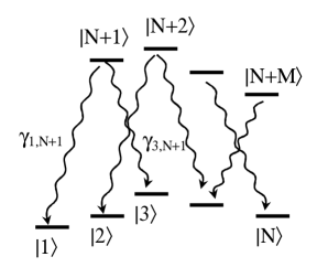
Figure 1: A general $N+M$ level quantum system with spontaneous emission rates between various energy levels.

II.2 Definitions of Purity

The density matrix is capable of describing any mixed state in quantum mechanics, ranging from pure states that are solutions of the TDSE, to completely incoherent states. There are several common ways of characterizing how close an arbitrary mixed state $\rho$ is to a pure state. These measures can be generally termed purity measures or purities. We use $P(\rho)$ to denote the purity of the density operator $\rho$.

The most common, and perhaps the simplest measure is $\rm{Tr}(\rho^{2})$ Messiah58 ; Bartana ; TannorRot ; Zeilinger . For any density matrix, $0<\rm{Tr}(\rho^{2})\leq 1$, with equality only for a pure state. Thus, the larger the value of Tr($\rho^{2}$), the closer a state is to being pure. Another useful measure is the von Neumann entropy, $S_{VN}=-k\ Tr(\rho\ln\rho)$ vonNeumann55 . The von Neumann entropy goes to zero for a pure state and is greater than zero for any mixed state, and thus the size of the von Neumann entropy is a measure of the degree of impurity of a state. Two other measures are the largest eigenvalue of $\rho$, $|\rho|_{\infty}$, which goes to 1 for a pure state and is less than one for a mixed state; and a measure based on the expansion of the characteristic equation for $\rho$, which has Tr($\rho^{2}$) as its leading term, but also takes into account higher order terms, e.g. Tr($\rho^{3}$) Byrd03 .

In general, as is apparent from the above discussion, the entire density matrix $\rho$ is not needed in order to characterize the purity of the system; rather, all that is necessary is the set of eigenvalues $\lambda$ of $\rho$. All purities can therefore be defined as functions solely of the eigenvalues, i.e

$$P(\rho)=P(\lambda(\rho)).$$ (4)

We will use the following definition of purity for the remaining part of the paper.

Definition 1

Given the density operator $\rho$, with spectrum $\lambda$, define its purity $P(\rho)$ as the largest eigenvalue of $\rho$, i.e.

$$P(\rho)=|\rho|_{\infty}=\lim_{n\to\infty}Tr(\rho^{n})^{1\over n}=\lambda^{\downarrow}_{1}.$$ (5)

Here $\lambda^{\downarrow}$ is the vector of eigenvalues of $\rho$ arranged in a decreasing order; for the remainder of this paper the superscript $\downarrow$ will be assumed every time $\lambda$ is written. Although many of the results in this paper are very general, we choose this measure as it gives simple answers for the cooling strategies. We will often use $P(\rho)$ or $P(\lambda)$ to mean the same thing, where it is understood that $\lambda$ is the spectrum corresponding to $\rho$.

II.3 Formulation of the Control Problem

The problem we address in this paper is the control of purity content of a quantum dissipative system which evolves under the LVN equation of motion given by eq. (1). The Hamiltonian $H[E]$ depends on an externaly controlled laser field $E(t)$ through the dipole coupling term. Beginning with the system in an initial mixed state it is required to find a control field functionality $E(t)$ that will drive the system through its equations of motion (1) to maximal purity, as defined by eq. (5), at some final time $T$.

The system evolution equation contains both a Hamiltonian part,

$$\dot{\rho}_{H}=-i[H[E],\rho],$$

and a dissipative part, given by

$$\dot{\rho}_{D}=L(\rho).$$

The Hamiltonian term leads to unitary evolution which does not change the spectrum, and the purity depends only on the spectrum. Thus, the dissipative term is required to obtain a purity increase. In TannorRot , the control problem was solved completely for the two-level system. In this paper we develop a formalism applicable to general $N$-level systems.

III Reformulation of the Control Problem in Terms of the Spectrum of $\rho$

III.1 Simplifying assumptions: complete and instantaneous unitary control

In this section we develop a general formalism that highlights the cooperative interplay between Hamiltonian and dissipative dynamics. Following TannorRot , we assume that the action of the control Hamiltonian can be produced on a time scale fast compared with spontaneous emission. This assumption is well established on physical grounds, since femtosecond laser control is now widely available and typical spontaneous emission times are nanosecond. In this paper we make an additional useful simplifying assumption about the dynamics, namely that the control Hamiltonian $H(t)$ can produce any unitary transformation $U\in SU(N)$ in the $N$ level system, i.e. the system of interest is unitarily controllable. Combining these two assumptions we have that any unitary transformation can be produced on the system in negligible time compared to the dissipation.

We use the notation

$$\o(\rho)=\{U\rho U^{\dagger}|U\in SU(N)\},$$

to denote the orbit of $\rho$ under unitary transformations. Since $\lambda(U\rho U^{{\dagger}})=\lambda(\rho)$, it is obvious that $P(\rho)=P(\lambda)$ is constant along the orbit $\o(\rho)$; however $\dot{P}$ is not: the rate of change of the purity due to dissipation is affected by where in $\o(\rho)$ the density matrix resides. In other words, due to the ’instantaneous controllability’ assumption, unitary controls can instantaneously direct $\rho$ along the orbit in order to change $\dot{P}$ in a controlled manner.

The above dynamical assumptions lead to another very important simplification. Since we have assumed that all unitary transformations in $SU(N)$ can be produced instantaneously, this includes bringing the density matrix into diagonal form. As a result, the different elements of each orbit can be considered redundant, and the orbit of $\rho$ can be completely represented by its diagonal form, or ’spectrum’, $\lambda(\rho)$. This suggests reformulating the control problem entirely in terms of the spectrum, rather than in terms of $\rho$ itself. The key step in this reformulation is to replace the equation of motion for $\rho$, eq. (1), with an equation of motion for the spectrum. We do this in the next section. As the purity is a function solely of the spectrum, this equation will allow the optimization to be performed just on the set of allowed spectra, significantly reducing the complexity of the problem. The controls will enter into this equation in a modified way that gives additional insight into the interplay of Hamiltonian and dissipative dynamics.

III.2 Equations of Motion for the Eigenvalues Assuming Fast Unitary Evolution

Suppose that $\rho$ has a nondegenerate spectrum, and let $\Lambda$ be its associated diagonal form. Consider two unitary transformations, $U_{1}$ and $U_{2}$. Then both $\rho_{1}=U_{1}\Lambda U_{1}^{\dagger}$ and $\rho_{2}=U_{2}\Lambda U_{2}^{\dagger}$ belong to $\o(\rho)$. However, they do not have the same spectrum after evolution under the dissipative dynamics. To understand how the spectrum of the density operator evolves, note that Hamiltonian dynamics produces no change in the spectrum. Therefore, the change in the spectrum is solely due to dissipation. After small time $\delta t$ the initial density operator $\rho$ evolves to

$$\rho\to\rho+L(\rho)\delta t,$$ (6)

If $\Lambda$ represents the diagonalization of the original density operator $\rho$ ($\rho=U\Lambda U^{\dagger}$, where $U$ is unitary) then the new density operator can be written as

$$\rho\to\rho+L(\rho)\delta t=U(\Lambda+U^{\dagger}L(U\Lambda U^{\dagger})U\delta t)U^{\dagger},$$ (7)

Consider now the change in spectrum under the evolution of eq. (7). Since $\Lambda$ is diagonal, the spectrum on the right hand side is, to first order in $\delta t$, just the diagonal i.e.

$$\lambda(t+\delta t)=diag(\Lambda+U^{\dagger}L(U\Lambda U^{\dagger})U\delta t).$$

Given the matrix $A$, the notation $diag(A)$ represents a vector whose entries are the diagonal entries of $A$. The rate of change of eigenvalues is then

$$\dot{\lambda}=diag(U^{\dagger}L(U\Lambda U^{\dagger})U)$$ (8)

which is in general different for different choices of $U$. Thus by applying varying unitary transformations $U$ and letting the dissipative dynamics evolve for some small time $\delta t$ we get different evolution of the spectrum. The unitary transformation should therefore be thought of as a control by which the spectrum of the density matrix can be affected.

III.3 Canonical decomposition

To proceed further, observe that the right hand side of eq. (8) describing the change in the spectrum under operation of the Lindbladian is a linear transformation on the vector of eigenvalues (see appendix A)

$$\dot{\lambda}=M\lambda.$$

To obtain an explicit expression for $M$ first note that for $U=I$ in eq. (8) we have $\dot{\lambda}=A\lambda$ with $A$ a $Q$-matrix (columns sum to zero) defined by $A_{ij}=\gamma_{ij}$ for $i\neq j$ and $A_{ii}=-\sum_{k}\gamma_{ki}$ otherwise. We split

$$A=B+D$$

where $D$ is the diagonal part of $A$ and is all non-positive whereas $B$ contains all off-diagonal entries and is all nonnegative. Using these definitions we get for general $U$ in eq. (8) (for details see appendix A):

$$\dot{\lambda}=(\Theta^{T}B\Theta+\Theta^{T}\circ D)\lambda,$$ (9)

where $\Theta_{ij}=|U_{ij}|^{2}$, is the Schur product of $U$ with its complex conjugate. Note that $\Theta$ has the important property of being a doubly-stochastic matrix (rows and columns all sum to unity). The notation $\Theta^{T}\circ D$ denotes the linear transformation of the diagonal of $D$ (as a vector) under the action of $\Theta^{T}$. In other words, if $d=diag(D)$, then $\Theta^{T}\circ D$ is a diagonal matrix whose diagonal is $\Theta^{T}d$. Note that in the special case where $U\in\{P_{i}\}$ — the set of permutations — $\Theta=P_{i}$, $P_{i}^{T}\circ D=P_{i}^{T}DP_{i}$ and hence eq.(9) simplifies to $\dot{\lambda}=\Theta^{T}A\Theta\lambda$.

Eq. (9) is one of the central results of this paper; it provides a reduced equation of motion for the spectral evolution under Lindblad dissipation and parametrized by the unitary control. From eq. (9), it is straightforward to infer, for example, that the eigenvalues of the density operator always remain nonnegative. In order to become negative an eigenvalue must pass through zero. If any of the eigenvalues $\lambda_{j}=0$, however, the only contributions to $\dot{\lambda}_{j}$ will be nonnegative since the only nonpositive elements in $M=\Theta^{T}B\Theta+\Theta^{T}\circ D$ reside on the diagonal. Hence none of the eigenvalues can turn negative.

III.4 Revised definition of the Control problem

Having formulated an equation of motion for the spectrum, eq. (9), we can now redefine the control problem in terms of the spectrum alone. We seek a control strategy in the form of a time varying unitary-stochastic matrix $\Theta(t)$ which when applied to the spectral equation of motion (9), will produce maximal purity $P(\lambda)$ at the final time $T$.

One strategy for choosing $\Theta(t)$ is to instantaneously maximize the purity $P(\lambda)$ at each point in time. Maximization algorithms that utilize this strategy are termed ’greedy’ algorithms and do not in general guarantee obtaining maximum possible purity at the final time $T$. To calculate the globally optimal cooling strategy we use the principle of dynamic programming Bertsekas87 , as described in the next section.

IV Dynamic Programming and the Hamilton-Jacobi-Bellman PDE

We now use the principle of dynamic programming for finding the optimal $\Theta(t)$ in Eq. (9). We will develop the basic ideas through the problem under consideration. Let $V(\lambda,t)$ denote the maximum achievable purity starting from initial eigenvalue spectrum $\lambda$ at time $t$ ($T-t$ units of time remaining). By definition of $V(\lambda,t)$, it is the maximum achievable purity if $\Theta$ is chosen optimally over the interval $[t,T]$. Suppose that at time $t$, the spectrum of $\rho(t)$ is $\lambda(t)$ and we make a choice of $\Theta(t)$. The resulting density operator after time $\delta t$ depends on the choice of $\Theta(t)$. The choice of $\Theta(t)$ should be such that for the resulting new spectrum $\lambda(t+\delta t)$, the return function, $V(\lambda(t+\delta t),t+\delta t)$ is maximized and by definition of the optimal return function should be same as $V(\lambda(t),t)$. By a Taylor series expansion we obtain

$$V(\lambda(t+\delta t),t+\delta t) = V(\lambda(t),t)+\frac{\partial V(\lambda,t)}{\partial t}\delta t$$ (10)

$$+\max_{\Theta}\langle\frac{\partial V(\lambda,t)}{\partial\lambda},\delta{\lambda}(\Theta)\rangle.$$

This then gives the well known Hamilton-Jacobi-Bellman PDE

$$\frac{dV(\lambda,t)}{dt}=\frac{\partial V(\lambda,t)}{\partial t}+\max_{\Theta}\langle\frac{\partial V(\lambda,t)}{\partial\lambda},\dot{\lambda}(\Theta)\rangle=0.$$ (11)

Observe that at the final time $T$, the value of the return function is just the purity of the density operator, i.e.

$$V(\lambda,T)=P(\lambda).$$

If we solve this PDE, together with its final condition, we will get the optimal control $\Theta$ as a function of the spectrum $\lambda$ and the time $t$, denoted as $\Theta=\Theta^{\ast}(\lambda,t)$. In other words, given the spectrum $\lambda$ of the density operator at time $t$, the best cooling strategy is to choose $\Theta^{\ast}(\lambda,t)$. This implies that the control problem is solved not just for a particular set of initial conditions; rather, it is embedded in a wider problem and a solution is sought simultaneously for all possible initial conditions.

In equation (11), the term $\frac{\partial V(\lambda,t)}{\partial t}$ has no dependence on $\Theta$, therefore

$$\Theta^{\ast}(\lambda,t)=\arg\max_{\Theta}\langle\frac{\partial V(\lambda,t)}{\partial\lambda},\dot{\lambda}(\Theta)\rangle.$$

Substituting for $\dot{\lambda}(\Theta)$ from Eq. (9), yields

$$\Theta^{\ast}(\lambda,t)=\arg\max_{\Theta}\langle\frac{\partial V(\lambda,t)}{\partial\lambda},(\Theta^{T}B\Theta+\Theta\circ D)\lambda\rangle.$$ (12)

Thus the problem reduces to finding the optimal control $\Theta^{\ast}(\lambda,t)$ that maximizes the expression

$$F(\Theta)\equiv\mu^{T}\left(\Theta^{T}B\Theta+\Theta^{T}\circ D\right)\lambda.$$ (13)

where the vector $\mu$ is defined as $\mu_{j}={\partial V\over\partial\lambda_{j}}$ (Although $\mu$ is a function of $\lambda$ and $t$, we just use $\mu$ and keep in mind that the dependence is implied). Note that a priori $V(\lambda,t)$ and hence $\mu$ are not known. However if we can make a guess at the optimal control strategy (which depends on $\lambda$ and $t$) and use this optimal strategy to integrate the equation of motion of the system evolution to obtain $V(\lambda,t)$ and hence $\mu$, then we can verify if the optimal control $\Theta$ and the corresponding $\mu$ satisfy equation (12). We illustrate this by finding optimal cooling strategies for a 3-level Lambda system.

The following properties of equation (13) will be used subsequently. $\Theta$ being a double stochastic matrix implies that $[1,1,...1]\Theta=[1,1,...1]$. Furthermore $[1,1,...1](B+D)=0$ and therefore $F(\Theta)$ vanishes for $\mu^{T}=[1,1,...,1]$. The elements of $\mu$ can therefore be shifted by a constant amount to make a specific component of $\mu$ vanish without influencing the value of $F(\Theta)$.

V Solution of the optimal control problem for the 3 level System

V.1 Preliminaries

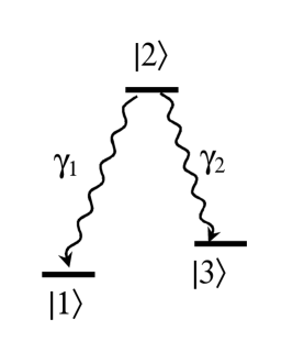
Figure 2: A 3 level Lambda system with spontaneous emission rate from level $2$ to $1$ given by $\gamma_{1}$ and spontaneous emission rate from $2$ to $3$ given by $\gamma_{2}$.

Consider a three level Lambda system depicted in figure 2. The excited state spontaneously decays into the stable ground states ${|{1}\rangle}$ and ${|{3}\rangle}$ at rate $\gamma_{1}$ and $\gamma_{2}$ respectively. We will assume without loss of generality that $\gamma_{1}\geq\gamma_{2}$.

The evolution of the density matrix of the three level Lambda system is given by

$$\dot{\rho}=-i[H(t),\rho] + \gamma_{1}(E_{1}\rho E_{1}^{\dagger}-\frac{1}{2}\{E_{1}^{\dagger}E_{1},\rho\})$$ (14)

$$+ \gamma_{2}(E_{2}\rho E_{2}^{\dagger}-\frac{1}{2}\{E_{2}^{\dagger}E_{2},\rho\}),$$

where $E_{1}={|{1}\rangle}{\langle{2}|}$ and $E_{2}={|{3}\rangle}{\langle{2}|}$. The equation of motion for the spectrum of the density matrix is then (9) with $A$, $B$ and $D$ given by

$$A=\left[\begin{array}[]{ccc}0&\gamma_{1}&0\\ 0&-(\gamma_{1}+\gamma_{2})&0\\ 0&\gamma_{2}&0\end{array}\right];$$

$$B=\left[\begin{array}[]{ccc}0&\gamma_{1}&0\\ 0&0&0\\ 0&\gamma_{2}&0\end{array}\right];\ \ D=\left[\begin{array}[]{ccc}0&0&0\\ 0&-(\gamma_{1}+\gamma_{2})&0\\ 0&0&0\end{array}\right].$$

The objective is to maximize the purity at time $T$, $P(T)$, as measured by the largest eigenvalue of $\rho$ (Definition 1).

V.2 The optimal strategy: Keep $\rho$ diagonal and ordered

Given the equation of motion defined by eq. 14 and the objective defined by Definition 1, we have the following theorem:

Theorem 1

The optimal cooling strategy For the 3-level system described above (labelled as in fig. 2) if any unitary transformation $U\in SU(3)$ can be produced in arbitrarily small time, then the optimal cooling strategy is to keep the density operator $\rho(t)$ diagonal for all times (produce no coherences) and ordered i.e. $\rho_{11}(t)\geq\rho_{22}(t)\geq\rho_{33}(t)$.

The optimal control strategy has the following alternate description. Throughout the cooling process, we keep the largest eigenvalue in the eigenstate ${|{1}\rangle}$, the next largest in state ${|{2}\rangle}$ and finally the smallest in state ${|{3}\rangle}$. As the population in state ${|{2}\rangle}$ decays spontaneously to state ${|{1}\rangle}$ and ${|{3}\rangle}$, after some time $\tau^{\ast}$, the population of states ${|{2}\rangle}$ and ${|{3}\rangle}$ will become equal. From that point onwards, we always maintain the population of states ${|{2}\rangle}$ and ${|{3}\rangle}$, equal (see figure 3).

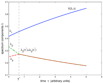
Figure 3: The eigenvalue evolution under the optimal cooling strategy for the three level $\Lambda$ system.

We will refer to this strategy as “greedy” since it maximizes the rate of increase of the objective at each point in time.

To prove optimality of the above strategy we proceed as follows. We first compute $V(\lambda,t)$ for the proposed strategy and then show that it satisfies the HJB equation maximized over all unitary transformations. Following the convention that the elements of the vector $\lambda$ are arranged in decreasing order, this amounts to showing that

$$I = \mathop{\rm argmax}_{\Theta\in\{|U|^{2}\ |\ U\in SU(N)\}}F(\Theta)$$ (15)

$$= \mathop{\rm argmax}_{\Theta\in\{|U|^{2}\ |\ U\in SU(N)\}}\mu^{T}\left(\Theta^{T}B\Theta+\Theta^{T}\circ D\right)\lambda,$$

where $I$ is the identity operator. This implies that the eigenvalues should be continuously maintained in their ordered arrangement. Note that despite the simplicity of this result, in general the continuous intervention of a control field is required in order that this condition be fulfilled.

V.3 The Return Function for the Ordered Diagonal Strategy

We now evaluate the return function for the putative optimal strategy. Let $\tau=T-t$ denote the remaining time for cooling. According to the strategy proposed above, two evolution regimes exist depending on whether $\tau\leq\tau^{\ast}$ or $\tau>\tau^{\ast}$, where $\tau^{\ast}$ is the critical time required for $\lambda_{2}$ and $\lambda_{3}$ to come to equilibrium.

In the case where $\tau\leq\tau^{\ast}$, under the proposed strategy the evolution equations of the system take the form

$$\dot{\lambda}_{1} = \gamma_{1}\lambda_{2}$$ (16)

$$\dot{\lambda}_{2} = -(\gamma_{1}+\gamma_{2})\lambda_{2}$$ (17)

$$\dot{\lambda}_{3} = \gamma_{2}\lambda_{2}$$ (18)

and therefore

$$V(\lambda,T-\tau)=\lambda_{1}+\frac{\gamma_{1}}{\gamma_{1}+\gamma_{2}}\lambda_{2}\left(1-e^{-(\gamma_{1}+\gamma_{2})\tau}\right);\ \ \tau<\tau^{\ast}.$$ (19)

By definition $\lambda_{2}(\tau^{\ast})=\lambda_{3}(\tau^{\ast})$ and $\lambda_{2}(\tau^{\ast})=\lambda_{2}e^{-(\gamma_{1}+\gamma_{2})\tau^{\ast}}$. Using these equalities, the following explicit forms for $\lambda_{2}(\tau^{\ast})$ and $\tau^{\ast}$ can be computed

$$\lambda_{2}(\tau^{\ast}) = \frac{\gamma_{2}\lambda_{2}+(\gamma_{1}+\gamma_{2})\lambda_{3}}{\gamma_{1}+2\gamma_{2}}.$$

$$\tau^{\ast} = -\frac{1}{\gamma_{1}+\gamma_{2}}\log\left(\frac{\lambda_{2}\gamma_{2}+\lambda_{3}(\gamma_{1}+\gamma_{2})}{\lambda_{2}(\gamma_{1}+2\gamma_{2})}\right).$$ (20)

After this point in time, under the ordered diagonal policy, the populations of states ${|{2}\rangle}$ and ${|{3}\rangle}$ are maintained at equilibrium such that $\lambda_{2}(\tau)=\lambda_{3}(\tau)=\frac{1}{2}(1-\lambda_{1}(\tau))$. The system dynamics therefore takes the form

$$\dot{\lambda}_{1}=-\frac{\gamma_{1}}{2}(1-\lambda_{1}),$$

from which the return function for the regime $\tau>\tau^{\ast}$, can be explicitly computed.

$$V(\lambda,T-\tau)=1-2\lambda_{2}(\tau^{\ast})e^{-\frac{\gamma_{1}}{2}(\tau-\tau^{\ast})};\ \ \tau>\tau^{\ast}.$$ (21)

As the return function enters the HJB equations only through its derivatives $\mu=\frac{\partial V}{\partial\lambda}$, we proceed to compute these derivatives explicitly for use in the next section.
For $\tau<\tau^{\ast}$, we have

$$\mu_{1} = 1$$

$$\mu_{2} = \frac{\gamma_{1}}{\gamma_{1}+\gamma_{2}}\left(1-e^{-(\gamma_{1}+\gamma_{2})\tau}\right)$$

$$\mu_{3} = 0$$ (22)

and for $\tau>\tau^{\ast}$, we have

$$\mu_{1} = 0$$

$$\mu_{2} = -\frac{2\gamma_{2}\lambda_{2}+\gamma_{1}\lambda_{3}}{\lambda_{2}(\gamma_{1}+2\gamma_{2})}e^{-\frac{\gamma_{1}}{2}(\tau-\tau^{\ast})}$$

$$\mu_{3} = -e^{-\frac{\gamma_{1}}{2}(\tau-\tau^{\ast})}$$ (23)

Note that in both regimes $\mu_{1}\geq\mu_{2}\geq\mu_{3}$, a property that will be used below. Also note that the $\mu$’s are continuous at $\tau=\tau^{\ast}$ up to a constant shift (see remark at the end of section IV).

V.4 Proof that the Return Function for the Ordered Diagonal Strategy Satisfies HJB

We proceed to calculate $\mathop{\rm argmax}F(\Theta)$ for $F(\Theta)$ given by eq. (13) and $\mu$ given by eq. (V.3) and (V.3). We show that $\Theta^{\ast}=I$ and hence the ordered diagonal strategy satisfies the HJB equation, proving that this strategy is globally optimal.

Absence of ground state coherences in the ordered diagonal solution

We first prove that the optimal transformation $\Theta$ in equation (13) has the property that $\Theta_{13}=\Theta_{31}=0$, namely that the ground state coherences vanish throughout the evolution of the optimal trajectory. Suppose $\Theta_{13}\neq 0$ and $\Theta_{31}\neq 0$ and say $\Theta_{31}\geq\Theta_{13}$. From equation (13) we have

$$\begin{split}F(\Theta)=&\left[\gamma_{1}(\mu_{1}\Theta_{11}+\mu_{3}\Theta_{13})+\gamma_{2}(\mu_{1}\Theta_{31}+\mu_{3}\Theta_{33})\right]\\ &\times\left[\lambda_{1}\Theta_{21}+\lambda_{2}\Theta_{22}+\lambda_{3}\Theta_{23}\right]\\ &-(\gamma_{1}+\gamma_{2})[\mu_{1}\lambda_{1}\Theta_{21}+\mu_{3}\lambda_{3}\Theta_{23}],\end{split}$$ (24)

where we have chosen $\mu_{2}=0$ and hence $\mu_{1}\geq 0\geq\mu_{3}$. Let $\Delta=\Theta_{13}$. Observe that in the above equation we can increase $\Theta_{11}$ and $\Theta_{33}$ by an amount $\Delta$ and decrease $\Theta_{13}$ and $\Theta_{31}$ by $\Delta$, to generate a new doubly stochastic matrix which gives a larger value of $F(\Theta)$ (this follows from the relations $\gamma_{1}\geq\gamma_{2}$ and $\mu_{1}\geq 0\geq\mu_{3}$). Hence we assume $\Theta_{13}=0$. Let $\Delta_{1}$ be the new value of $\Theta_{31}$. Now if we increase $\Theta_{11}$ and $\Theta_{32}$ by $\Delta_{1}$ and decrease $\Theta_{31}$ and $\Theta_{12}$ by the same amount we get a new doubly stochastic matrix which gives a larger value of $F(\Theta)$. Hence we need to maximize $F(\Theta)$ only over those doubly stochastic matrices for which $\Theta_{13}=\Theta_{31}=0$.

Dependence of $F(\Theta)$ on the remaining parameters in $\Theta$

As the rows and columns of $\Theta$ must sum to unity there remain only two degrees of freedom in the components of $\Theta$. Therefore, we can write $F(\Theta)$ as a function of only two of its components:

$$F(\Theta) = F(\Theta_{21},\Theta_{23})$$ (25)

$$= \left[\gamma_{1}\mu_{1}(1-\Theta_{21})+\gamma_{2}\mu_{3}(1-\Theta_{23})\right]$$

$$\times\left[\lambda_{2}+\Theta_{21}(\lambda_{1}-\lambda_{2})+\Theta_{23}(\lambda_{3}-\lambda_{2})\right]$$

$$-(\gamma_{1}+\gamma_{2})\left[\mu_{1}\Theta_{21}\lambda_{1}+\mu_{3}\Theta_{23}\lambda_{3}\right].$$

It is now required to find the maximum of $F(\Theta_{21},\Theta_{23})$ on the triangular domain $0\leq\Theta_{21}\leq 1$, $\quad 0\leq\Theta_{23}\leq 1$, $\Theta_{21}+\Theta_{23}\leq 1$.

The maximum cannot lie at an interior point.

Suppose $F$ has a maximum in the interior, then the Hessian of $F$ at that point must be negative definite. We proceed to show that the Hessian $G_{ij}\equiv\frac{\partial^{2}F}{\partial\Theta_{2i}\partial\Theta_{2j}}$, with $i,j=\{1,3\}$, is not negative definite anywhere and therefore the maximum must reside on the boundary. Computing the components of $G$ we find

$$G_{11} = -2(\lambda_{1}-\lambda_{2})\mu_{1}\gamma_{1}$$

$$G_{33} = -2(\lambda_{3}-\lambda_{2})\mu_{3}\gamma_{2}$$

$$G_{31} = G_{13}=-\mu_{1}(\lambda_{3}-\lambda_{2})\gamma_{1}-\mu_{3}(\lambda_{1}-\lambda_{2})\gamma_{2}.$$ (26)

Denoting $a\equiv\gamma_{1}\mu_{1}(\lambda_{3}-\lambda_{2})$ and $b\equiv\gamma_{2}\mu_{3}(\lambda_{1}-\lambda_{2})$, the determinant of $G$ is $4ab-(a+b)^{2}=-(a-b)^{2}\leq 0$ such that one of the eigenvalues of $G$ is non negative and therefore $G$ is not negative definite.

The maximum point is $(\Theta_{21},\Theta_{23})=(0,0).$

As the maximum does not reside in the interior of the triangular domain it must lie on one of the edges $[(0,0),(0,1)]$, $[(0,0),(1,0)]$ or $[(0,1),(1,0)]$.

It can be shown by checking the first and second derivatives along the edge $[(0,1),(1,0)]$ that the maximum along that interval lies at the end point $(\Theta_{21},\Theta_{23})=(0,1)$. We now check the remaining two edges. As $G_{11}$ and $G_{33}$ are both non positive it follows that $F(\Theta)$ is concave in both the $\Theta_{21}$ and $\Theta_{23}$ directions. Therefore, if in addition the slope at the point $(0,0)$ is negative in both directions, this establishes the existence of a maximum at that point. We proceed to show that indeed the slopes are non negative:

$$\left.\frac{\partial F}{\partial\Theta_{21}}\right|_{(0,0)} = (\lambda_{1}-\lambda_{2})[\mu_{3}\gamma_{2}+\mu_{1}\gamma_{1}]+\lambda_{2}[-\mu_{1}\gamma_{1}]$$ (27)

$$-(\gamma_{1}+\gamma_{2})\mu_{1}\lambda_{1}\leq 0$$

$$\left.\frac{\partial F}{\partial\Theta_{23}}\right|_{(0,0)} = (\lambda_{3}-\lambda_{2})[\mu_{3}\gamma_{2}+\mu_{1}\gamma_{1}]+\lambda_{2}[-\mu_{3}\gamma_{3}]$$ (28)

$$-(\gamma_{1}+\gamma_{2})\mu_{3}\lambda_{3}\leq 0.$$

The first expression follows from the fact that $\gamma_{1}\geq\gamma_{2}$, $\mu_{1}\geq 0\geq\mu_{3}$ and $\lambda_{1}\geq\lambda_{2}$. The second expression can be proved by inserting the explicit forms for $\mu$, eq. (V.3) and (V.3), for the two regimes of $T-t$.

VI Discussion and Conclusions

We have presented a general framework for calculating optimal purity increasing strategies in $N$ level dissipative systems under the assumption of complete and instantaneous unitary control. In so doing, we derived a reduced equation of motion for the spectral evolution under dissipation and parametrized by the unitary control. The Hamilton-Jacobi-Bellman Theorem was invoked to provide sufficient criteria for global optimality. This general framework was then explicitly applied to derive and prove optimality of the greedy cooling strategy for a three level $\Lambda$ system.

In future work we intend to apply this methodology to obtain explicit optimal cooling strategies for general $N+M$ level systems comprised of $M$ excited states coupled to $N$ ground states. One is tempted, by extrapolation from the present results, to assume that the greedy algorithm should be optimal in general and hence that coherences do not play a role in the optimal cooling strategy for $N>3$. However, preliminary numerical results based on dynamical programming show that the greedy algorithm is in general not optimal in these systems. Rather, a strategy based on “delayed gratification” is superior to the greedy strategy, and coherences play a small but finite role in these larger systems. This will be the subject of a future paper.

Appendix A Derivation of the ’Canonical form’

We wish to show that eq. (8) is a linear transformation of the form

$$\dot{\lambda}=M\lambda.$$

Recall first that

$$\begin{split}U^{\dagger}&L(U\Lambda U^{\dagger})U\\ &=\sum_{ij}\gamma_{ij}U^{\dagger}\left[{|{i}\rangle}{\langle{j}|}U\Lambda=U^{\dagger}{|{j}\rangle}{\langle{i}|}-\frac{1}{2}\left\{{|{j}\rangle}{\langle{j}|},U\Lambda U^{\dagger}\right\}\right]U\\ &=\sum_{ij}\gamma_{ij}\left[U^{\dagger}{|{i}\rangle}{\langle{j}|}U\Lambda U^{\dagger}{|{j}\rangle}{\langle{i}|}U-\frac{1}{2}\left\{U^{\dagger}{|{j}\rangle}{\langle{j}|}U,\Lambda\right\}\right]\end{split}$$

Expanding eq. (8) and rewriting it in component form we have

$$\dot{\lambda}_{k} = \sum_{ij}\gamma_{ij}\left[\sum_{s}U^{\dagger}_{ki}U_{js}\lambda_{s}U^{\dagger}_{sj}U_{ik}\right.$$ (29)

$$\quad\quad\quad\left.-\frac{1}{2}\{U^{\dagger}_{kj}U_{jk}\lambda_{k}+\lambda_{k}U^{\dagger}_{kj}U_{jk}\}\right]$$

$$= \sum_{s}\left[\sum_{ij}\Theta^{T}_{ki}\gamma_{ij}\Theta_{js}-\sum_{j}\Theta^{T}_{kj}\sum_{i}\gamma_{ij}\delta_{ks}\right]\lambda_{s}$$

$$\equiv \sum_{s}M_{ks}\lambda_{s},$$

with

$$M\equiv\Theta^{T}B\Theta+\Theta^{T}\circ D,$$

and with the definitions of $\Theta$, $B$, $D$ and the operation $\Theta\circ D$ as provided in the main text. Rewriting the above in vector format we have precisely eq. (9)

$$\dot{\lambda}=(\Theta^{T}B\Theta+\Theta^{T}\circ D)\lambda.$$

References

- (1) D. J. Tannor and S. A. Rice, J. Chem. Phys. 83, 5013 (1985).
- (2) D. J. Tannor, R. Kosloff, and S. A. Rice, J. Chem. Phys. 85, 5805 (1986).
- (3) D. J. Tannor and S. A. Rice, Adv. Chem. Phys. 70, 441 (1988).
- (4) R. Kosloff, S. A. Rice, P. Gaspard, S. Tersigni, and D. J. Tannor, Chem. Phys. 139, 201 (1989).
- (5) S. A. Rice and M. Zhao, Optical Control of Molecular Dynamics, Wiley, New York, 2000.
- (6) M. Shapiro and P. Brumer, Principles of the Quantum Control of Molecular Processes, Wiley, New York, 2003.
- (7) T. Brixner and G. Gerber, Chem. Phys. Chem. 4, 418 (2003).
- (8) R. Mitrić, M. Hartmann, J. Pittner, and V. Bonačić-Koutecký, J. Phys. Chem. A 106, 10477 (2002).
- (9) A. P. Peirce, M. A. Dahleh, and H. Rabitz, Phys. Rev. A 37, 4950 (1988).
- (10) S. Shi and H. Rabitz, Comp. Phys. Commun. 63, 71 (1991).
- (11) W. Jakubetz and J. Manz, Chem. Phys. Lett. 165, 100 (1990).
- (12) H. Shen, J. P. Dussault, and A. D. Bandrauk, Chem. Phys. Lett. 221, 498 (1994).
- (13) Y. J. Yan, R. E. Gillilan, R. M. Whitnell, K. R. Wilson, and S. Mukamel, J. Chem. Phys. 97, 2320 (1993).
- (14) N. Khaneja, R. Brockett, and S. J. Glaser, Phys. Rev. A 63, 032308 (2001).
- (15) T. Hornung, S. Gordienko, R. de Vivie-Riedle, and B. Verhaar, Phys. Rev. A 66, 043607 (2002).
- (16) S. E. Sklarz and D. J. Tannor, Phys. Rev. A 66, 053619 (2002).
- (17) S. E. Sklarz, I. Friedler, D. J. Tannor, Y. B. Band, and C. J. Williams, Phys. Rev. A 66, 053620 (2002).
- (18) C. Rangan and P. H. Bucksbaum, Phys. Rev. A 64, 033417 (2001).
- (19) C. M. Tesch, L. Kurtz, and R. de Vivie-Riedle, Chem. Phys. Lett. 343, 633 (2001).
- (20) J. P. Palao and R. Kosloff, Phys. Rev. Lett. 89, 188301 (2002).
- (21) M. Leibscher, I. S. Averbukh, and H. Rabitz, Phys. Rev. Lett. 90, 213001 (2003).
- (22) H. Rabitz, R. de Vivie-Riedle, M. Motzkus, and K. Kompa, Science 288, 824 (2000).
- (23) R. J. Gordon and S. A. Rice, Annu. Rev. Phys. Chem. 48, 601 (1997).
- (24) A. Bartana, R. Kosloff, and D. J. Tannor, J. Chem. Phys. 99, 196 (1993).
- (25) A. Bartana, R. Kosloff, and D. J. Tannor, J. Chem. Phys. 106, 1435 (1997).
- (26) D. J. Tannor and A. Bartana, J. Phys. Chem. A. 103, 10359 (1999).
- (27) J. S. Cao, M. Messina, and K. R. Wilson, J. Chem. Phys. 106, 5239 (1997).
- (28) P. Gross and S. D. Schwartz, J. Chem. Phys. 109, 4843 (1998).
- (29) Y. Ohtsuki, K. Nakagami, W. Zhu, and H. Rabitz, Chem. Phys. 287, 197 (2003).
- (30) N. Khaneja, T. Reiss, B. Luy, and S. J. Glaser, Journal of Magnetic Resonance 162, 311 (2003).
- (31) G. Lindblad, Commun. Math. Phys. 33, 305 (1973).
- (32) R. Alicki and K. Lendi, Quantum Dynamical Semigroups and Applications, Springer, New York, 1986.
- (33) A. Messiah, Quantum Mechanics, volume 1, Wiley, New York, 1958.
- (34) C. Brukner and A. Zeilinger, Phys. Rev. Lett. 83, 3354 (1999).
- (35) J. von Neumann, Mathematical Foundations of Quantum Mechanics, Princeton University press, Princeton, N.J., 1955.
- (36) M. S. Byrd and N. Khaneja, Notes on group invariants and positivity of density matrices and superoperators, arXive:quant-ph/0302024, 2003.
- (37) A. W. Marshall and I. Olkin, Theory of majorization and its applications, Academic Press, New York, 1979.
- (38) R. Bhatia, Matrix analysis, Springer, New York, 1997.
- (39) D. P. Bertsekas, Dynamic programming and optimal control, Athena Scientific, Belmont, Massachusetts, 1987.