Spontaneous emission of homogeneous broadening molecules on a micro-droplet’s surface and local-field correction

Abstract

We consider the spontaneous emission of a broadening molecule on the surface of a micro-sphere in this paper. The density of states for the micro-cavity is derived from quasi-normal models(QNM’s) expansion of the correlation functions of electromagnetic fields. Through detailed analysis we show that only weak coupling between a broadening atom(molecule) and the electromagnetic fields exists in a dielectric sphere cavity whether the sphere is small or big. From these results we find the explicit expression of the spontaneous emission decay rate for a surfactant broadening molecule on the surface of a micro-droplet with radius $a$, in which only $1/a$ and $1/a^{2}$ components exhibit. Then we apply this expression to a real experiment and obtain a consistent result with the experiment. We also show that the real-cavity model of local field correction is accurate, and reveal that the local-field correction factor can be measured precisely and easily by fluorescence experiments of surfactant molecules. Moreover, the spontaneous decay of a surfactant molecular on droplet’s surface is sensitive to the atomic broadening, so that the fluorescence experiment in a micro-sphere cavity can be used to estimate the radiative broadening.

I Introduction

It is well known that the spontaneous emission of an atom or a molecule is not an intrinsic atomic property, but rather results from the coupling of an atom or a molecule to the electromagnetic environment. PurcellPurcell noted first that the spontaneous radiate rate can be enhanced if an atom is placed in a cavity. Kleppner studied the opposite caseKleppner , i.e. inhibited spontaneous emission may happen in some conditions. Cavity quantum electrodynamics is just to investigate the effects of electromagnetic boundary conditions on atomic or molecular radiative properties. A micro-sphere is easily made in experiment not only by liquid but also by solid and acts as a cavityChang ; Kimble1 . In this cavity many optical phenomena, such as fluorescence, lasing, and many nonlinear optical processes, have been intensively studied and a great progress has also been achieved over the past two decades. Recently, a great attention has been paid to the fluorescence from spherical droplets ($\mu m$) due to a plenty of application. In addition, the micro-droplet can be applied to biology as a biosensorArnold02 ; Arnold03 to detect a protein molecule. Up to now, many studies have been made on fluorescence properties of dye molecules in a micro-cavity Arnold1 ; Arnold2 ; Arnold3 ; Vos1 . It has been observed that the fluorescence decay rate shows a pronounced dependence on a droplet radius. In particular, a surfactant molecule may be naturally localized at the surface of liquid droplets. Their spontaneous emission decay exhibits characteristicsArnold2 that were thought very much puzzling at least in the past. When the diameter of a droplet is larger than $15\mu m$, the spontaneous emission decay rate is a constant and much smaller than that in bulk material. But this result cannot be explained satisfactorily so far. We note that Arnold $et\ al$ have made some valuable exploring and achieved important progress toward to explaining the experimental resultsArnold4 ; Arnold5 . We also note Wu’sWu work on this topic.
Recently, there has been much interest in the spontaneous emission decay of an atom or a molecule embedded in material even in dispersive and absorbing dielectricWelsch1 . Both theoretical and experimental studies have been made. Since in reality the atom embedded in dielectric is in a small region of free space, the local field ’felt’ by the atom is different from that in the continuous medium. The decay rate is modified by local field correction factor. Different models have been used to calculate it. The typical models are virtual-cavity modelV-cavity1 and real-cavity modelGlauber1 ; Tomas . The recent experiments have been reported, from which the real-cavity model may be favoredR-cavity1 ; R-cavity2 . But the virtual-cavity model is appropriate to describe interstitial gest atoms of the same kind as the host continuentsV-cavity2 , i.e. only one kind of atom or molecule is present.
It is notable that the experimental result obtained by Barnes $et\ al$Arnold2 is normalized to the decay rate of rhodamine B that is dissolved in the bulk glycerol. This decay rate obviously contains affections of the medium so that the local field correction cannot be ignored. But the surfactant molecule is located on the air-liquid boundary, so there is no local field correction in this case. On the other hand, in the experiment done by Barnes $et\ al$ the emission moment orientation of surfactant molecules is always in the tangent direction of the surface of a glycerol droplet, and therefore the fluorescence emission of the dye molecule is in fact a two-dimension system, which is considered necessary in studying its spontaneous emission decay.
With the help of quasi-normal modes(QNM’s) expansion Leung2 for electric field in a sphere, we first in this paper derive the density of states, which is a Lorentzian shape. Then we start from the basic equations of a two-level molecule interacting with electromagnetic fields in full quantum theory framework. From detailed analysis we conclude that there is no strong coupling when a homogeneous broadening atom or molecule is located inside or on the surface of a micro-sphere. Only weak coupling exists in the system even if the size of a sphere is very large. Taking these into consideration, we calculate the explicit expression of spontaneous emission decay rate for a homogenous broadening atom or molecule in a cavity with Lorentzian resonance modes. Using this result and the sum rule of the density of states, we get the very simple explicit expression of the spontaneous emission decay rate when a molecule is on the surface of a sphere, which indeed contains both ($1/a$) and ($1/a^{2}$) componentsArnold3 . Finally, we take the local-field correction (real-cavity model) into account and draw a theoretical curve which is in agreement with the experimental result. The asymptotical constant of the decay rate for large diameter is related to the local- field correction factor, which is dependent only on the refractive index of the droplet. This result not only verifies the accuracy of the local-field correction factor but also shows that the fluorescence experiment of a surfactant molecule on the surface of a sphere provides a good means of measuring local-field correction factor. In addition, we show that the fluorescence experiment in a micro-sphere is sensitively dependent on the radiative broadening of atomic spectrum. This kind of experiment can estimate the spectrum broadening.
The present paper is organized as follows. In Section II, we derive the density of states of the electromagnetic field on the surface of a sphere. The decay rate of a homogeneous broadening atom or molecule in any cavity with Lorentzian mode is given in Section III. In Section IV, we apply the general result to expressing explicitly the dependence of the fluorescence decay rate on the sphere radius and present a numerical result. Some discussions are presented in Section V.

II Density of states on a droplet’s surface

II.1 Electromagnetic QNM’s

In solving the electromagnetic problems in a dielectric sphere, the quasinormal models(QNM’s) that satisfy the out-going wave boundary condition at infinity and correspond the morphology-dependent resonance(MDR’s) are very useful physical concept and convenient mathematical toolLeung2 . For a perfect sphere, the electromagnetic fields can be expanded by QNM’s and divided into two parts, one is TE mode

$${\bf e}_{1jlm}({\bf r})=\frac{f_{1jl}}{r}{{\bf X}_{lm}}$$ (2.1)

and the other is TM mode

$${\bf e}_{2jlm}({\bf r})=\frac{1}{\omega_{2j}\epsilon(r)}\nabla\times\left[\frac{f_{2jl}}{r}{\bf X}_{lm}\right]$$ (2.2)

where $\epsilon(r)$is the dielectric constant, ${\bf X}_{lm}$ are vector spherical harmonics with angular momentum quantum number $l$ and magnetic quantum number $m$. $f_{\mu jl}(\mu=1,2)$ are called QNM’s wave functions and satisfy the following equation($c=1$)Leung1

$$\frac{d}{dr}\beta(r)\frac{df}{dr}+\beta(r)\left[\epsilon(r)\omega^{2}-\frac{l(l+1)}{r^{2}}\right]f(r)=0$$ (2.3)

where $\beta(r)=1$ for TE modes and $\beta(r)=1/\epsilon(r)$ for TM modes. $f_{\mu jl}$ are complete and orthogonal for different $j$Liusy . The sum rules

$$\sum_{j}\frac{f_{\mu jl}(r)f_{\mu jl}(r^{{}^{\prime}})}{\omega_{\mu j}}=\sum_{j}\frac{f_{\mu jl}(r)f_{\mu jl}(r^{{}^{\prime}})}{\omega_{\mu j}^{3}}=\cdots=0$$ (2.4)

are very useful. We will use them later.

II.2 Density of states

By means of QNM’s, one can expand the correlation functions. It is easy to showHo1

$${\rho}(\omega)=\frac{1}{\pi}F_{E}({\bf r,r},\omega)$$ (2.5)

where ${\rho}(\omega)$ is the density of states. In the free space, it is well known that

$${\rho}_{0}(\omega)=\frac{\omega^{3}}{\pi^{2}c^{3}}$$ (2.6)

$F_{E}({\bf r,r},\omega)$ is the sum of vacuum fluctuation of the electric field for all components

$${\rho}(\omega) = \frac{1}{\pi}\sum_{i}F_{Eii}({\bf r,r},\omega)$$ (2.7)

$$= \omega^{2}{\rm Im}\sum_{lj}\frac{{\bf e}_{\mu jlm}({\bf r})\cdot{\bf e}_{\mu jlm}^{\dagger}({\bf r})}{\omega_{jl}(\omega-\omega_{jl})}$$

where ${\bf e}_{\mu jlm}^{\dagger}({\bf r})$ is the conjugate vector of ${\bf e}_{\mu jlm}({\bf r})$, in which only ${\bf X}_{lm}$ is replaced by ${\bf X}_{lm}^{*}$. QNM’s eigenfunctions for a fixed $l$ are given by

$$f_{j}(r)=\left\{\begin{array}[]{cc}C_{j}rj_{l}(n_{0}\omega_{j}r)&\mbox{}\hskip 28.45274pt0<r<a\\ B_{j}rh_{l}^{(1)}(\omega_{j}r)&\mbox{}\hskip 45.5244ptr>a\end{array}\right.$$ (2.10)

The coefficients $C_{j}$ are

$$C_{j}^{2}=\left\{\begin{array}[]{ll}\left[a^{3}(n_{0}^{2}-1)j_{l}(n_{0}\omega_{j}a)/2\right]^{-1}&\mbox{}\hskip 11.38109pt{\rm TE\ case}\\ \left[a^{3}(n_{0}^{2}-1)S/2\right]^{-1}&\mbox{}\hskip 11.38109pt{\rm TM\ case}\end{array}\right.$$ (2.13)

where

$$S=\frac{1}{n_{0}^{2}}\left\{\left[\frac{j_{l}^{{}^{\prime}}(n_{0}\omega_{j}a)}{j_{l}(n_{0}\omega_{j}a)}+\frac{1}{n_{0}\omega_{j}a}\right]^{2}+\frac{l(l+1)}{(\omega_{j}a)^{2}}\right\}$$ (2.14)

and

$$B_{j}=C_{j}j_{l}(n_{0}\omega_{j}a)/h_{j}^{(1)}(\omega_{j}a)$$ (2.15)

In the above equations, the resonance frequency $\omega_{j}$ is complex

$$\omega_{j}=\omega_{j0}+i\omega_{jI}$$ (2.16)

The real part is the resonance frequency of MDR’s and the imaginary part is half of the full width at half maximum(HFWHM) of these resonances. We can rewrite $\omega_{j}$ as the common form

$$\omega_{j}=\omega_{j0}+i\frac{\gamma_{lj}}{2}$$ (2.17)

The electric field for TE mode is only along the tangent of droplet’s surface. Using (2.7) and sum rules (2.4), we can get the density of states

$${\rho}(\omega) = \sum_{lj}\frac{2l+1}{4\pi^{2}}\frac{2\omega}{a^{3}(n_{0}^{2}-1)}\frac{1}{\omega_{jI}}\frac{(\omega_{jI})^{2}}{(\omega-\omega_{j0})^{2}+(\omega_{jI})^{2}}$$

$$= \sum_{lj}{\rho}_{0}(\omega)\frac{2l+1}{(n_{0}^{2}-1)x^{2}}\frac{1}{\gamma_{lj}^{x}}\frac{(\gamma_{lj}/2)^{2}}{(\omega-\omega_{lj})^{2}+(\gamma_{lj}/2)^{2}}$$

$$\approx {\rho}_{0}(\omega)\sum_{lj}\frac{2l+1}{(n_{0}^{2}-1)x_{lj}^{2}}\frac{1}{\gamma_{lj}^{x}}\frac{(\gamma_{lj}^{x}/2)^{2}}{(x-x_{lj})^{2}+(\gamma_{lj}^{x}/2)^{2}}.$$

where $x$, $x_{lj}$ and $\gamma_{lj}^{x}$ are the dimension-free variables(restore $c$)

$$x = \frac{\omega}{c}a$$

$$x_{lj} = \frac{\omega_{j0}}{c}a$$

$$\gamma_{lj}^{x} = \frac{\gamma_{j0}}{c}a$$ (2.19)

$x_{lj}$ and $\gamma_{lj}^{x}$ are independent of sphere radius $a$ and $\gamma_{lj}^{x}$ augment along with $j$ for a fixed $l$ and are given asymptotically byLeung1

$$\gamma_{l\infty}^{x}=\frac{1}{n_{0}}ln\frac{n_{0}+1}{n_{0}-1}$$ (2.20)

So the density of states on the surface of a sphere is the standard Lorentzian distribution. For a given $l$ there are infinity resonance modes, but only several resonance modes ahead ($j=1,2,3\dots$) are important because these resonance widths are narrower and the resonance points $x_{lj}$ are smaller.

III Basic equations and their solutions

Ten years agoLeung3 , Lai $et\ al$ studied the spontaneous decay rate of a two-level atom in a cavity with Lorentzian modes and discussed the conditions of weak coupling, strong coupling and intermediate coupling. In this section, we still use the same method and investigate the radiative properties of a homogeneous broadening molecule. We consider a system that is composed of an atom, electromagnetic fields(cavity) and their interaction. The atom, which has two energy levels, a lower level $a$ and upper level $b$, is located at position ${\bf r_{0}}$ in a cavity. The interaction Hamiltonian between the atom and the electric field is

$$\mbox{\unboldmath{V}}={\mu\cdot E(r_{0})}$$ (3.1)

where ${\bf\mu}$  is the electric dipole operator and $\bf E$ is the electric field. We assume that an excited atom is initial at upper level $|b\rangle$ and $C(t)$ denotes it’s amplitude. The other related state of the system is described by $|as\rangle$ with amplitude $D_{s}(t)$, in which the atom is at the lower atomic state $|a\rangle$ and one photon is in mode $s$. In interaction representation and under the rotating wave approximation, one can obtain usual Wigner-Weisskopf equationLeung3 ; Heitler

$$i\hbar\frac{dC(t)}{dt}=\sum_{s}V_{s}^{*}D_{s}e^{i(\Omega-\omega_{s})t}$$ (3.2)

$$i\hbar\frac{dD_{s}(t)}{dt}=V_{s}C(t)e^{-i(\Omega-\omega_{s})t}$$ (3.3)

where $\hbar\Omega=E_{b}-E_{a}$ and $V_{s}=\langle as|V|b\rangle$. After some algebraic calculations, it is easy to get

$$\frac{dC(t)}{dt}=-\frac{2\pi}{\hbar}\frac{M}{3}\int\limits_{0}^{\infty}d\omega{\rho}(\omega)\int_{0}^{t}d\tau C(\tau)e^{i(\Omega-\omega)(t-\tau)}$$ (3.4)

where

$$M=\langle a|\mu_{i}|b\rangle\langle b|\mu_{i}|a\rangle$$ (3.5)

and $\rho(\omega)$ is the density of states at position ${\bf r_{0}}$ in the cavity. The factor $3$ appears in (3.4) because we have assumed that the atomic dipole matrix element is isotopic and has equal probability in any direction in 3-dimension space.
For complex molecules or homogeneous broadening atoms, the fluorescence spectrum is band-type, so one must consider a large number of lower levels $a_{1},a_{2},\cdots$ forming a continuum. Then the amplitude of the probability that the atom is in up state should satisfy

$$\frac{dC(t)}{dt} = -\frac{2\pi}{\hbar}\frac{1}{m}\int\limits_{0}^{+\infty}d\omega{\rho}(\omega)$$ (3.6)

$$* \int\limits_{0}^{+\infty}d\Omega\int_{0}^{t}d\tau C(\tau)M(\Omega)e^{i(\Omega-\omega)(t-\tau)}$$

where $m$ is the number of freedom degree of the atomic dipole in a cavity and $M(\Omega)$ is atomic dipole matrix element per unit transition frequency. In practical cases, the diople moment of an atom or a molecule is not free in every direction, so we must introduce this parameter $m$. Assuming that the line shape of atomic braodening is Lorentzian distribution

$$M(\Omega)=M_{0}\frac{\Gamma_{h}}{2\pi}\frac{1}{(\Omega-\Omega_{0})^{2}+(\frac{\Gamma_{h}}{2})^{2}}$$ (3.7)

we now derive that the strong coupling condition when a broadening atom is in a sphere cavity. Considering the ideal case, i.e. the maximum coupling $\Omega_{0}=\omega_{0}$, one can regard the cavity as a single mode cavity

$$\rho(\omega)=\rho_{0}K\frac{(\frac{\gamma}{2})^{2}}{(\omega-\omega_{0})^{2}+(\frac{\gamma}{2})^{2}}$$ (3.8)

where

$$K=\frac{2l+1}{n_{0}^{2}-1}\frac{1}{x_{0}^{2}}\frac{1}{\gamma^{x}}$$ (3.9)

Then $C(t)$ satisfies

$$\frac{dC(t)}{dt}=\int_{0}^{t}d\tau S(t-\tau)C(\tau)$$ (3.10)

where the kernel $S$ is

$$S(t-\tau)=-\frac{K\gamma}{4\tau_{0}}e^{-\frac{1}{2}(\Gamma_{h}+\gamma)(t-\tau)}$$ (3.11)

$\tau_{0}$ is the spontaneous decay lifetime in vacuum

$$\tau_{0}=\frac{4M_{0}\Omega_{0}^{3}}{3\hbar c^{3}}$$ (3.12)

It is easy to find

$$\frac{d^{2}C(t)}{dt^{2}}+\frac{1}{2}(\Gamma_{h}+\gamma)\frac{dC(t)}{dt}+\frac{K\gamma}{4\tau_{0}}C(t)=0$$ (3.13)

The strong coupling should satisfy the following conditionLeung3

$$\frac{K\gamma}{\tau_{0}}\gg\left(\frac{\Gamma_{h}+\gamma}{2}\right)^{2}\approx\frac{\Gamma_{h}^{2}}{4}$$ (3.14)

Given $x_{0}=\Omega_{0}a/c$, when $l\approx n_{0}x_{0}$(the least leaky mode)Leung1 ; Leung4 , the enhanced factor $K$ in (3.9) will be maximum

$$K_{max}=\frac{2n_{0}}{n_{0}^{2}-1}\frac{1}{x_{0}}\frac{1}{\gamma^{x}}$$ (3.15)

the strong coupling condition reduces

$$\left(\frac{\Gamma_{h}}{c}\right)^{2}\ll\frac{8n_{0}}{n_{0}^{2}-1}\frac{1}{x_{0}a\tau_{0}c}$$ (3.16)

In visible light domain, $\tau_{0}\sim 10^{-9}s$, $a\sim 10\mu m$ and $x_{0}\sim 100$, the above inequality becomes

$$\left(\frac{\Gamma_{h}}{c}\right)^{2}\ll 10(cm^{-1})$$ (3.17)

So the strong coupling will be exhibited only when $\Gamma_{h}<1cm^{-1}$, which is very difficult to be met in experiment because the typical value of the homogeneous broadening is $100cm^{-1}$. If the atomic broadening is in the order of $\Gamma_{h}\sim 10cm^{-1}$, the interaction between an atom or a molecule and a spherical cavity must be weak coupling.
For Rydberg’s atom, $\tau_{0}\sim 10^{-2}s$, $a\sim 1cm$ and $x_{0}\sim 100$, the strong coupling condition is changed into

$$\left(\frac{\Gamma_{h}}{c}\right)^{2}\ll 10^{-8}(cm^{-1})$$ (3.18)

Which is also very difficult to be satisfied. So we can conclude that there is no strong coupling between a broadening atom and microsphere cavity modes.
Under the weak coupling case, it is significant only for $t-\tau\rightarrow 0$ in the integration of (3.6), so that it becomes Markovian

$$\frac{dC(t)}{dt}\approx-\left[\frac{\gamma}{2}+i\delta\right]C(t)$$ (3.19)

and

$$\frac{\gamma}{2}+i\delta=\frac{2\pi}{\hbar}\frac{1}{m}\int d\omega\int d\Omega\frac{{\rho}(\omega)M(\Omega)}{i(\omega-\Omega-i\epsilon)}$$ (3.20)

We assume that $\rho(\omega)$ is still Lorentzian

$$\rho(\omega)=\rho_{0}\sum_{j}K_{j}\frac{(\frac{\gamma_{j}}{2})^{2}}{(\omega-\omega_{j})^{2}+(\frac{\gamma_{j}}{2})^{2}}$$ (3.21)

Substituting (3.7) and above equation into (3.20), we have

$$\frac{\gamma}{2} = \rho_{0}\frac{2\pi^{2}}{\hbar}\frac{M_{0}\Gamma_{h}}{2m\pi}\sum_{j}K_{j}$$ (3.22)

$$*\int\limits_{0}^{+\infty}d\omega\frac{(\frac{\gamma_{j}}{2})^{2}}{(\omega-\omega_{j})^{2}+(\frac{\gamma_{j}}{2})^{2}}\frac{1}{(\omega-\Omega_{0})^{2}+(\frac{\Gamma_{h}}{2})^{2}}$$

$$= \frac{1}{\tau_{0}}\frac{3}{8m}\sum_{j}K_{j}\gamma_{j}\frac{\Gamma_{h}+\gamma_{j}}{(\Omega_{0}-\omega_{j})^{2}+(\frac{\Gamma_{h}+\gamma_{j}}{2})^{2}}$$

$$= \frac{1}{\tau_{0}}\frac{3}{2m}\sum_{j}K_{j}\gamma_{j}\frac{\Gamma_{h}+\gamma_{j}}{(2\Delta_{j})^{2}+(\Gamma_{h}+\gamma_{j})^{2}}$$

where $\Delta_{j}=\Omega_{0}-\omega_{j}$ and we have used the integration formula

$$\int\limits_{0}^{+\infty}d\omega\frac{1}{(\omega-\omega_{j})^{2}+(\frac{\gamma_{j}}{2})^{2}}\frac{1}{(\omega-\Omega_{0})^{2}+(\frac{\Gamma_{h}}{2})^{2}}$$

$$=\frac{2\pi}{\gamma_{j}\Gamma_{h}}\frac{\Gamma_{h}+\gamma_{j}}{(\Omega_{0}-\omega_{j})^{2}+(\frac{\Gamma_{h}+\gamma_{j}}{2})^{2}}$$ (3.23)

in which we have assumed $\gamma_{j},\Gamma_{h}\ll\omega_{j},\Omega$, so that the integral can be evaluated by integrating over the whole real line.
The spontaneous emission decay rate of a homogeneous broadening molecule in the cavity is finally written in the following form

$$\frac{\gamma}{\gamma_{0}^{vac}}=\frac{3}{m}\sum_{j}K_{j}\gamma_{j}\frac{\Gamma_{h}+\gamma_{j}}{(2\Delta_{j})^{2}+(\Gamma_{h}+\gamma_{j})^{2}}$$ (3.24)

where $\gamma_{0}^{vac}=1/{\tau_{0}}$ is the decay rate of the molecule in vacuum. For resonance case $\Delta_{j}=0$ and if the cavity mode spacing is much larger than $\Gamma_{h}$, only one cavity mode is important and then the decay rate can be approximately expressed as

$$\frac{\gamma}{\gamma_{0}^{vac}}\approx\frac{3}{m}\frac{K\gamma}{(\Gamma_{h}+\gamma)}$$ (3.25)

Letting $\delta_{c}$ be the cavity modes separation and using the sum rule Ching1 ; Yokoyama1

$$K\gamma\approx\delta_{c}$$ (3.26)

we can obtain the two limiting cases for m=3

$$\frac{\gamma}{\gamma_{0}^{vac}}=\left\{\begin{array}[]{ll}K\mbox{}\hskip 56.9055pt\Gamma_{h}\ll\gamma\\ \delta_{c}/\Gamma_{h}\mbox{}\hskip 39.83385pt\Gamma_{h}\gg\gamma\end{array}\right.$$ (3.29)

which are just the common results of weak couplingYokoyama1 . The above equations are held only when the atom is resonated in a cavity and the cavity mode spacing is much larger than the resonance width of a cavity mode. But (3.24) is a accurate expression of spontaneous emission decay rate for a broadening molecule in a cavity under the weak coupling condition.
Generally speaking, the enhanced factor $K_{j}$ satisfies $K_{j}=K_{j}^{0}/\gamma_{j}$, so that $K_{j}\gamma_{j}=K_{j}^{0}$ is independent of $\gamma_{j}$ and then

$$\frac{\gamma}{\gamma_{0}^{vac}}=\frac{3}{m}\sum_{j}\frac{K_{j}^{0}}{\gamma_{j}^{{}^{\prime}}}\frac{(\gamma_{j}^{{}^{\prime}}/2)^{2}}{(\Omega_{0}-\omega_{j})^{2}+(\gamma_{j}^{{}^{\prime}}/2)^{2}}$$ (3.30)

where $\gamma_{j}^{{}^{\prime}}=\gamma_{j}+\Gamma_{h}$. This means that the spontaneous emission decay rate is formally proportional to the density of fields states but the resonance width is replaced by the sum of a cavity mode width and the broadening of a molecule’s energy level, which may be very useful to the analysis of the decay rate of a homogeneous broadening molecule in practice.
In the following section, we shall concentrate on spherical cavities and explain the experimental result.

IV Spherical cavities cases

We now apply the general results of the former section to a homogeneous broadening molecule in a spherical cavity. For a dielectric sphere, the expression (III) of the decay rate is given by the following form

$$\frac{\gamma}{\gamma_{0}^{vac}}=\frac{3}{m}\sum_{li}K_{li}\gamma_{li}^{x}\frac{\Gamma_{h}^{x}+\gamma_{li}^{x}}{(2\Delta x_{li})^{2}+(\Gamma_{h}^{x}+\gamma_{li}^{x})^{2}}$$ (4.1)

In the practical experiment, the result is normalized to the decay rate of rhodamine B in bulk glycerol. But $\gamma_{0}^{vac}$ is the decay rate of a broadening molecule in vacuum. In order to compare the theoretical result with the experimental data, both sides of the above equation should be divided by the factor $n_{0}\xi_{lc}$ and then

$$\frac{\gamma}{\gamma_{0}} = \frac{1}{n_{0}\xi_{lc}}\frac{3}{m}\sum_{li}K_{li}\gamma_{li}^{x}\frac{\Gamma_{h}^{x}+\gamma_{li}^{x}}{(2\Delta x_{li})^{2}+(\Gamma_{h}^{x}+\gamma_{li}^{x})^{2}}$$ (4.2)

$$= \left.\frac{1}{n_{0}\xi_{lc}}\frac{3}{m}\frac{\rho_{c}(x_{0})}{\rho_{0}}\right|_{\gamma_{li}^{x}\rightarrow\gamma_{li}^{x}+\Gamma_{h}^{x}}$$

where $\xi_{lc}$ is the local-field correction factor and according to real-cavity model Welsch1 ; Glauber1 it reads

$$\xi_{RC}=\left(\frac{3n_{0}^{2}}{2n_{0}^{2}+1}\right)^{2}$$ (4.3)

Because the surfactant molecule is on the surface of a sphere, the field ’felt’ by a surfactant molecule is the same as the macro-field on the surface of a sphere, so there is no local-field correction for the decay rate of a surfactant molecule in this case. From (4.2), it is easy to see that the peak values of the spontaneous emission decay rate are all at the positions of MDR’s, but the widths are much larger than those of MDR’s. Dye molecules are of multi-atom molecules so that the fluorescence spectrum is very wide. For octadecyl rhodamine B used by Barns $et\ al$Arnold2 in their experiment, the center of its fluorescence spectrum is at $\lambda_{0}=560nm$ with the band width of $\Delta\lambda=60nm$. Within the band width, we note that the interresonance separation is about $\delta_{c}^{x}=0.7$Leung4 for a spherical cavity with $n_{0}=1.47$. Therefore 3 or more transitions are resonance transitions, in which the transition probabilities are much larger than those non-resonance transitions. So the spontaneous emission decay rate is determined mainly by these resonance transitions, in which the corresponding transition probabilities are increased with the decrease of the transition wave length. It is a good approximation to choose the decay rate of a dye molecule whose the resonance transition is near $\lambda_{0}$ as the average value of all resonance transitions. On the other hand, the directions of a surfactant molecular dipole moment are always along the tangency of the sphere so that $m=2$ and then TE mode is much more significant than TM mode for spontaneous emission. In (4.2), because $\delta_{c}^{x}\gg\gamma_{li}^{x}+\Gamma_{h}^{x}$, the least leaky cavity mode ($i=1$ and $l\approx n_{0}x_{0}$) is the most important for given $x_{0}=x_{li}$, the other parts can be regarded as ’background’

$$\left.\frac{\rho_{c}(x_{0})}{\rho_{0}}\right|_{\gamma_{li}^{x}\rightarrow\gamma_{li}^{x}+\Gamma_{h}^{x}}=\gamma_{b}+\frac{K_{l1}\gamma_{l1}^{x}(\Gamma_{h}^{x}+\gamma_{l1}^{x})}{(2\Delta x_{l1})^{2}+(\Gamma_{h}^{x}+\gamma_{l1}^{x})^{2}}$$ (4.4)

where the second term in the above equation is the contribution of the least leaky TE resonance mode that is near to $x_{0}$, while the first term $\gamma_{b}$ is called ’background’, in which all TE modes and the tangent parts of TM modes are included except the least leaky TE resonance mode $x_{l1}$.
On the surface of a sphere, the density of states is redistributed and the sum rule Ching1

$$\int\limits_{x_{0}-\delta_{c}^{x}/2}^{x_{0}+\delta_{c}^{x}/2}dx_{0}\frac{\rho_{c}(x_{0})}{\rho_{0}}=\delta_{c}^{x}$$ (4.5)

is still valid, because $\delta_{c}^{x}\gg\gamma_{li}^{x}+\Gamma_{h}^{x}$. Here $\delta_{c}^{x}$ is the cavity mode spacing . Substituting (4.4) into the above equation, one can easily show

$$\gamma_{b}=1-\frac{\pi}{2}\frac{K_{l1}\gamma_{l1}^{x}}{\delta_{c}^{x}}$$ (4.6)

Using (II.2), we have

$$K_{l1}\gamma_{l1}^{x} = \frac{2l+1}{n_{0}^{2}-1}\frac{1}{x_{l1}^{2}}$$ (4.7)

$$\approx \frac{2n_{0}}{n_{0}^{2}-1}\frac{1}{x_{0}}$$

and then

$$\frac{\gamma}{\gamma_{0}}=\frac{1}{n_{0}\xi_{lc}}\frac{3}{2}\left[1+\frac{2n_{0}}{n_{0}^{2}-1}\frac{1}{x_{0}}\left(\frac{1}{\Gamma_{h}^{x}}-\frac{\pi/2}{\delta_{c}^{x}}\right)\right]$$ (4.8)

where we have omitted $\gamma_{l1}^{x}$ and let $m=2$. If we let

$$x_{0} = \frac{2\pi}{\lambda_{0}}a=\alpha a$$ (4.9)

$$\Gamma_{h}^{x} = \frac{\Gamma_{h}}{c}a=\frac{2\pi\Delta\nu_{s}}{c}a=\beta a$$ (4.10)

where $a$ will be in the unit of $\mu m$ later. (4.8) is rewritten as the following form

$$\frac{\gamma}{\gamma_{0}}=\frac{1}{n_{0}\xi_{lc}}\frac{3}{2}\left[1+\frac{2n_{0}}{n_{0}^{2}-1}\frac{1}{\alpha}\left(\frac{1}{\beta a^{2}}-\frac{\pi/2}{\delta_{c}^{x}}\frac{1}{a}\right)\right]$$ (4.11)

In the above equation, there are $1/a$ and $1/a^{2}$ components, the result of which is in agreement with what was obtained by ArnoldArnold4 .
Arnold estimates from their experiment that the homogeneous broadening of rhodamine B in glycerol is $\Delta\nu=100cm^{-1}$Arnold2 ; Arnold4 . Because the surfactant molecule is on the surface of droplets of glycerol, it is reasonable to think that the homogeneous broadening of a surfactant molecule is only half of that in bulk glycerol. If we take $\Delta\nu_{s}=50cm^{-1}$, $\beta=0.0314$. The other parameter $\alpha=11.2$ for $\lambda_{0}=560nm$. The refractive index of glycerol is $n_{0}=1.47$. By means of these parameters, we can easily get the decay rate for any size spherical cavity. Fig.1 is the numerical result. In Fig.1, the three curves correspond to three different local-field correction factors. The experimental data show that the local-field correction is slightly less ($90\%-95\%$) than that of real-cavity model. This difference maybe coming from the fact that the size of the dye molecule is much bigger than single atom molecule, so that the local-field correction factor of the real-cavity model is just a good approximation. The affections of the molecular shape should be taken into account for this case.

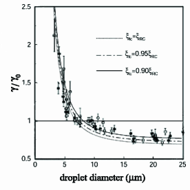
Figure 1: The spontaneous emission decay rate of octadecyl rhodamine B on the surface of a glycerol droplet as a function of droplet size. Three curves correspond to the three different local-field correction factors. We take $\Delta\nu_{s}=50cm^{-1}$ in Eq.(4.10). The experimental data are from Ref.Arnold2 .

From (4.11), the local-field correction factor is connected easily with the experimental result

$$\xi_{lc}=\frac{3}{2n_{0}g}$$ (4.12)

where

$$g=\lim_{a\rightarrow\infty}\frac{\gamma}{\gamma_{0}}$$ (4.13)

If one measures the decay rate of surfactant molecules on the surface of a larger sphere, the local-field correction factor is then given by (4.12). This reveals that the fluorescence experiment of surfactant molecules is a good approach to measure precisely and conveniently the local-field correction factor, which was not recognized and is out of what we have predicted before.
In (4.8), apart from $\Gamma_{h}$, other parameters are determined only by the refractive index $n_{0}$, in which $\delta_{c}^{x}$ is derived from Mie’s theoryLeung4 . What we have chosen in Fig.1 for $\Gamma_{h}$ is based on the above analysis. In fact, the decay rate is very sensitive to $\Gamma_{h}$ because $\beta$ is in the component of $1/a^{2}$ and then the room where $\Gamma_{h}$ may be chosen in this experiment is very small. The numerical calculations show that $\Gamma_{h}$ in Fig.1 is really the best. So this experiment is also a good method to measure or estimate at least the homogeneous broadening of a molecule.

V Conclusions and discussions

In the present paper we have considered the spontaneous emission decay rate of a broadening atom or molecule in a cavity. For a broadening molecule, it is very difficult to exhibit the strong coupling between molecule and fields in a cavity to happened. We have proved by detailed analysis that there is no strong coupling in a dielectric sphere cavity. Under the weak coupling condition, we obtained the exact expression of spontaneous emission decay rate for a broadening molecule in any cavity with Lorentzian mode distribution and discussed the two common limiting cases. Simply speaking, the decay rate of spontaneous emission for a homogeneous broadening molecule equals the density of states, in which the widths of the cavity resonance modes are replaced by the sum of cavity mode width and the broadening of a atomic energy level. Applying this general formula to a spherical cavity, we have a simple analytical expression that shows explicitly the dependence of the fluorescence decay rate on the spherical radius. When we explain the experimental resultArnold2 , two points are important: one is that the freedom degree of the surfactant molecule transition dipole moment is $2$ and the other is the local-field correction factor. Moreover, QNM’s expansion of the fields is very convenient to obtain the density of states for a spherical cavity. The sum rule of the density of states plays a very important role in simplifying the result and in numerical calculation. Finally, it is noted that new significance of the fluorescence experiment on the surface of droplets is revealed in our present work. This kind of experiment is a very good method to measure precisely the local-field correction factor.
We gratefully acknowledge helpful discussions with Prof. S. Arnold. Y-J. Xia and G-C. Guo were supported by the National Fundamental Research Program (2001CB309300), National Natural Science Foundation of China, and the Innovation funds from the Chinese Academy of Sciences.

References

- (1) E. M. Purcell, Phys. Rev. 69, 681(1946).
- (2) D. Kleppner, Phys. Rev. Lett. 47, 233(1987).
- (3) For a review on microsphere, see Optical Processes in Microcavities, edited by R. K. Chang and A. J. Campillo(World Scientific, Singapore, 1996).
- (4) D. W. Vernooy, A. Furusawa, N. P. Georgiades, V. S. Ilchenko, and H. J. Kimble, Phys. Rev. A57, 2293(1998).
- (5) F. Vollmer, D. Braun, A. Libchaber, M. Khoshsima, I. Teraoka and S. Arnold, Appl. Phys. Lett. 80, 4057(2002).
- (6) S. Arnold, M. Khoshsima, I. Teraoka, S. Holler and F. Vollmer Opt. Lett. 28, 272(2003).
- (7) M. D. Barnes, W. B. Whitten, S. Arnold, and J. M. Ramsey, J. Chem. Phys 97, 7842(1992).
- (8) M. D. Barnes, C-Y. Kung, W. B. Whitten, J. M. Ramsey, S. Arnold and S. Holler, Phys. Rev. Lett. 76, 3931(1996).
- (9) H. Yukawa, S. Arnold, and K. Miyano, Phys. Rev. A60, 2491(1999).
- (10) M. Megens, J. E. G. J. Wijnhoven, A. Lagendijk, and W. L. Vos, Phys. Rev. A59,4727(1999).
- (11) S. Arnold, J. Chem. Phys. 106, 8280(1997).
- (12) S. Arnold, S. Holler, and N. Goddard, Mater. Sci. Eng., B48, 139(1997).
- (13) Y. Wu, Phys. Rev. A61,33803(2000).
- (14) S. Scheel, L. Knöll, and D. -G. Welsch, Phys. Rev. A60, 4094(1999).
- (15) J. Knoester and S. Mukamel, Phys. Rev. A40, 7065(1989).
- (16) R. J. Glauber and M. Lewenstein, Phys. Rev. A43, 467(1991).
- (17) M. S. Tomas, Phys. Rev. A63, 53811(2001).
- (18) G. L. J. A. Rikken and Y. A. R. R. Kessener, Phys. Rev. Lett. 74, 880(1995).
- (19) F. J. P. Schuurmans, D. T. N. de Lang, G. H. Wegdam, R. Sprik, and A. Lagendijk, Phys. Rev. Lett. 80, 5077(1998).
- (20) P. de Vries and A. Lagendijk, Phys. Rev. Lett.81, 1381(1998).
- (21) For a review on QNM’s, see E. S. C. Ching, P. T. Leung, A. Maassen van den Brink, W. M. Suen, S. S. Tong and K. Young, Rev. of Mod. Phys, 70, 1554(1998).
- (22) P. T. Leung and K. M. Pang, J. Opt. Soc. Am. B13, 805(1996).
- (23) P.T. Leung, S. Y. Liu, and K. Young, Phys. Rev. A49, 3057(1994).
- (24) K. C. Ho, P. T. Leung, A. M. van den Brink, and K. Young, Phys. Rev. E58, 2965(1998).
- (25) H. M. Lai, P. T. Leung and K. Young, Phys. Rev. A37, 1597(1989).
- (26) W. Heitler, The Quantum Theory of Radiation, 3rd ed. (Oxford, Clarendon,1954).
- (27) P. T. Leung and K. Young, J. Opt. Soc. Am. B9, 1585(1992).
- (28) S. C. Ching, H. M. Lai and K. Young, J. Opt. Soc. Am. B4, 1995(1989).
- (29) H. Yokoyama and S. D. Brorson, J. Appl. Phys. 66, 4801(1989).