Relativistic Scattering with a Singular Potential in the Dirac Equation

Abstract

An elementary treatment of the Dirac equation in the presence of a three dimensional spherically symmetric delta potential is presented. We show how to calculate the cross section using the relativistic wave expansion method for a one delta potential and two concentric delta potentials. We compare our results with the cross section calculated in the Born approximation.

I Introduction

The non relativistic scattering theory, and in particular the partial wave expansion method, is a very well known issue. An extensive literature cohen exists in this subject. In the relativistic case, however, the scattering problem with a potential, has almost not been discussed. This has to do, probably, with the fact that relativistic quantum mechanics is, in fact, a theory of many particles and, therefore, quantum field theory is a more appropriate language to discuss these kind of problems.

We think, however, that the scattering problem in the frame of the Dirac equation deserves some attention. This fact has motivated us to make use of a simple mathematical method, valid for central potentials, the so called relativistic partial wave expansion method provides us with valuable information for relativistic particles near the low energy limit, giving us also values for the phase shifts and cross section of the scattered wave for different channels of the angular momentum. This method will be used to complement the work done in loewe , a discussion for bound states in the presence of a delta potential, which shows how to fix the boundary conditions for the wave function when crossing the $V(r)=a\delta(r-r_{0})$ potential. We will like to remark that there are general treatments for boundary conditions for this kind of singular potentials, in the frame of the construction of self adjoint extensions for the Dirac Hamiltonian dittrich .

In this work we use the relativistic partial wave expansion method with the boundary conditions mentioned above, making a simple analysis for the scattering states. Moreover, we will also introduce a double delta potential of the form $V(r)=\pm a_{1}\delta(r-r_{1})\pm a_{2}\delta(r-r_{2})$.

The idea is to discuss the behavior of the differential and total cross section when we vary the energy of the incident particles, analyzing the occurrence of certain resonances in different channels. We also find a useful relationship between the phase shifts and the total cross section.

This work is complemented with the use of the Born approximation, that gives us a more general perspective of this problem.

II Relativistic scattering

As it is extremely well known, asymptotically, we expect that the wave function in the non relativistic case will behave as

$$\Psi(r)\textrm{\tiny$r\tilde{\rightarrow}\infty$}\exp{(iKz)}+f(\theta,\phi)\frac{\exp{(iKr)}}{r}.$$ (1)

where $K$ is the momentum. The differential cross section is then

$$I(\theta,\phi)=\frac{d\sigma}{d\Omega}=|f(\theta,\phi)|^{2}.$$ (2)

For scattering at high energies of 1/2-spin particles, we must consider the Dirac equation

$$(c\hat{\alpha}\cdot\hat{p}+\hat{\beta}mc^{2}+V(r))\psi(r)=H\psi(r),$$ (3)

where $\hat{\alpha}$ and $\hat{\beta}$ are the usual $4x4$ Dirac matrices, and $\psi$ is the four-component Dirac spinor.

We know that for a free particle, the one dimensional solution of the above equation is

$$\Psi=\sqrt{\frac{\epsilon+mc^{2}}{2\epsilon}}\left(\begin{array}[]{c}\chi_{\sigma}\\ \frac{\sigma_{z}p}{\epsilon+mc^{2}}\chi_{\sigma}\end{array}\right)e^{i(p_{z}z-\epsilon t)},$$ (6)

where $\epsilon=\pm E_{p}$, $\sigma=\pm 1$, $\chi_{1}=\left(\begin{array}[]{c}1\\ 0\end{array}\right)$, $\chi_{-1}=\left(\begin{array}[]{c}0\\ 1\end{array}\right)$ and $\sigma_{z}=\left(\begin{array}[]{cc}1&0\\ 0&-1\end{array}\right)$.

When working with a spherical symmetric potential it is better to transform the Dirac equation into spherical coordinates greiner ; rose , where the complete set of commuting operators is given by $H$, $J^{2}$, $J_{3}$ and $\kappa$, where $\hat{J}$ is the total angular momentum and $\hat{\kappa}$ is defined by

$$\hat{\kappa}=\beta(\frac{2}{\hbar}\hat{S}\cdot\hat{L}+\hbar 1).$$ (7)

The eigenvalues of the operator $\kappa$ are given by

$$\hat{\kappa}\Psi=-\kappa\hbar\Psi=\pm(j+\frac{1}{2})\hbar\Psi,$$ (8)

If we parametrize the four-component spinor by separating the radial and angular dependence according to the Ansatz

$$\Psi=\left(\begin{array}[]{cc}g(r)&\chi^{\mu}_{\kappa}(\theta,\phi)\\ if(r)&\chi^{\mu}_{-\kappa}(\theta,\phi)\end{array}\right),$$ (9)

where

$$\chi^{\mu}_{\kappa}=\sum_{m}C(l\frac{1}{2}j;\mu-m;m)Y^{\mu-m}_{l}\chi^{m},$$ (10)

being $C(l\frac{1}{2}j;\mu-m;m)$ are the appropriate Glebsch-Gordan coefficients. It is easy to see that the $\hat{\kappa}$ operator satisfies the following relationship with the angular momentum-spin function

$$\hat{\kappa}\chi^{\mu}_{\kappa}=-\kappa\chi^{\mu}_{\kappa},$$

$$\hat{\kappa}\chi^{\mu}_{-\kappa}=\kappa\chi^{\mu}_{-\kappa}.$$ (11)

For the two different coupling, $j=l+1/2$ and $j=l-1/2$, the eigenvalues are given by

$$\kappa=\left\{\begin{array}[]{lll}l&j=l-1/2&\kappa>0\\ -l-1&j=l+1/2&\kappa<0\end{array}.\right.$$ (14)

The dependence of $\kappa$ on the eigenvalues of the angular momentum will be extremely important for our calculations. Everything will be function of $\kappa$. However, in the future we will replace $\kappa$ with the respective $l_{\kappa}$ remembering the existence of the LS coupling. We notice that:

$$l_{\kappa}=\left\{\begin{array}[]{ll}\kappa&\kappa>0\\ -\kappa-1&\kappa<0\end{array}.\right.$$ (17)

and

$$l_{-\kappa}=\left\{\begin{array}[]{ll}\kappa-1&\kappa>0\\ -\kappa&\kappa<0\end{array}.\right.$$ (20)

The Dirac equation in spherical coordinates has the form

$$\left(-ic\hat{\alpha}_{r}\left(\frac{\partial}{\partial r}+\frac{1}{r}-\frac{\hat{\beta}}{r}\hat{\kappa}\right)+\hat{\beta}mc^{2}+V(r)\right)\Psi(r)=E\Psi(r).$$ (21)

The solution of this equation for a free particle with the Ansatz given in (9) is:

$$G(r)=r(a_{1}j_{l_{\kappa}}(r)+b_{1}n_{l_{\kappa}}(r)),$$ (22)

$$F(r)=\frac{\kappa}{|\kappa|}\frac{k\hbar c}{E+mc^{2}}r(a_{1}j_{l_{-\kappa}}(r)+b_{1}n_{l_{-\kappa}}(r)).$$ (23)

where $G(r)=rg(r)$, $F(r)=rf(r)$ and $j_{l}$, $n_{l}$ are the regular and irregular Bessel functions respectively.

III Partial wave expansion method

Here we will present the relativistic wave expansion method. The reader can see the details in dapor . This method shows us how to calculate the differential and total cross section just by knowing the phase shift of the scattered wave.

Let us consider the asymptotic behavior of a 1/2-spin scattered wave

$$\begin{array}[]{cc}\Psi_{i}=a_{i}\exp{(iKz)}+b_{i}(\theta,\phi)\frac{\exp{(iKr)}}{r}&i=1,...,4\end{array}.$$ (24)

To be able to find the effects of the scattering in the spin of the particle, we must first notice that not all the components of the spinor that represents the free particle are independent, which, in turns, allows us to see that not all the $b_{i}(\theta,\phi)$ components are independent. For example if we have a spin parallel to the direction of incidence (spin up), we have:

$$\Psi_{1}\textrm{\tiny$r\tilde{\rightarrow}\infty$}\exp{(iKz)}+f^{+}(\theta,\phi)\frac{\exp{(iKr)}}{r},$$ (25)

$$\Psi_{2}\textrm{\tiny$r\tilde{\rightarrow}\infty$}g^{+}(\theta,\phi)\frac{\exp{(iKr)}}{r}.$$ (26)

Now, if the spin is anti-parallel to the direction of incidence (spin down) we have

$$\Psi_{1}\textrm{\tiny$r\tilde{\rightarrow}\infty$}g^{-}(\theta,\phi)\frac{\exp{(iKr)}}{r},$$ (27)

$$\Psi_{2}\textrm{\tiny$r\tilde{\rightarrow}\infty$}\exp{(iKz)}+f^{-}(\theta,\phi)\frac{\exp{(iKr)}}{r}.$$ (28)

The functions $f^{\pm}(\theta,\phi)$ and $g^{\pm}(\theta,\phi)$ are called scattering amplitudes (similar to the non relativistic case). With these amplitudes we can calculate the differential cross section for a non polarized beam, making the change $f^{+}=f^{-}=f$, $g^{+}=g\exp{(i\phi)}$ and $g^{-}=-g\exp{(-i\phi)}$ getting

$$I(\theta,\phi)=\frac{d\sigma}{d\Omega}=|f|^{2}+|g|^{2},$$ (29)

where the new scattering amplitudes are given by

$$f(\theta)=\sum_{l=0}^{\infty}\hat{A}_{l}P_{l}(\cos{\theta}),$$ (30)

$$g(\theta)=\sum_{l=1}^{\infty}\hat{B}_{l}P^{1}_{l}(\cos{\theta}),$$ (31)

and

$$\hat{A}_{l}=\frac{1}{2iK}\{(l+1)[\exp{(2i\eta^{+}_{l})}-1]+l[\exp{(2i\eta^{-}_{l})}-1]\},$$ (32)

$$\hat{B}_{l}=\frac{1}{2iK}[\exp{(2i\eta^{-}_{l})}-\exp{(2i\eta^{+}_{l})}].$$ (33)

We can see that the differential cross section has a direct dependence on the phase shifts of the wave function. The notation $\eta_{l}^{\pm}$ gives us the dependence of the wave function on the angular momentum and on the two different coupling ($j=l\pm 1/2$). It is easy to calculate the total cross section, just by integrating the differential cross section, obtaining

$$\sigma_{total}=4\pi\sum_{l}\frac{|\hat{A}_{l}|^{2}+l(l+1)|\hat{B}_{l}|^{2}}{2l+1}.$$ (34)

IV 1-Delta potential

As we mentioned before, we will apply the wave expansion method to a spherical potential given by

$$V(r)=\pm a\delta(r-r_{0}).$$ (35)

To be able to find the phase shifts, in order to obtain the differential and total cross section, we must use the boundary conditions described in loewe :

$$F^{2}_{+}+G^{2}_{+}=F^{2}_{-}+G^{2}_{-},$$ (36)

and

$$\frac{F_{+}}{G_{+}}=\frac{(F_{-}/G_{-})+\alpha}{1-\alpha(F_{-}/G_{-})},$$ (37)

where $F_{+}$ y $G_{+}$ are the solutions of the Dirac equation outside the potential ($r>r_{0}$), and $F_{-}$ y $G_{-}$ are the solutions inside the potential ($r<r_{0}$). $\alpha$ is an dimensionless constant that involves the constant $a$, $\alpha\equiv\tan{(a/\hbar c)}$.

The first boundary condition tells us that the absolute value of a function with real part $F$ and imaginary part $G$ is constant, which is nothing but the continuity of the probability density. The second boundary condition will be essential to calculate the phase shifts.

First we must find the solution of the Dirac equation in all regions of space. Since we are dealing with a delta type potential, it will only influence the wave function in the support $r=r_{0}$, being, therefore, the solution is the same as in the free particle case. Separating the space in two regions:

I.- For $r<r_{0}:$

$$G_{1}(r)=ra_{1}j_{l_{\kappa}}(kr),$$ (38)

$$F_{1}(r)=\frac{\kappa}{|\kappa|}\frac{k\hbar c}{E+mc^{2}}a_{1}j_{l_{-\kappa}}(kr).$$ (39)

The functions $n_{l_{\kappa}}(kr)$ and $n_{l_{-\kappa}}(kr)$ do not appear in the above equation, because the wave function must remain finite at the origin.

II.- For $r>r_{0}$

$$G_{2}(r)=r(j_{l_{\kappa}}(kr)\cos(\eta^{\pm}_{l})-n_{l_{\kappa}}(kr)sen(\eta^{\pm}_{l})),$$ (40)

$$F_{2}(r)=\frac{\kappa}{|\kappa|}\frac{k\hbar c}{E+mc^{2}}(j_{l_{-\kappa}}(kr)\cos(\eta^{\pm}_{l})-n_{l_{-\kappa}}sen(\eta^{\pm}_{l})).$$ (41)

Here we have written $a_{2}$ and $b_{2}$ as the phase shifts of the scattered wave. These phase shifts can be found using the boundary conditions. Equation (36) does not give us much valuable information. It only allows us to find the constant $a_{1}$ in the wave functions. We will concentrate on the second boundary condition (37). Here the constant $a_{1}$ disappear, leaving us $\eta^{\pm}_{l}$ as the only variable. A simple algebra gives us:

$$\tan(\eta^{\pm}_{l})=\frac{\alpha(A^{2}j^{2}_{l_{-\kappa}}+j^{2}_{l_{\kappa}})}{A(n_{l_{-\kappa}}j_{l_{\kappa}}-n_{l_{\kappa}}j_{l_{-\kappa}})+\alpha(n_{l_{\kappa}}j_{l_{\kappa}}+A^{2}n_{l_{-\kappa}}j_{l_{-\kappa}})},$$ (42)

where

$$A=\frac{\kappa}{|\kappa|}\frac{k\hbar c}{E+mc^{2}}.$$ (43)

The spherical Bessel functions can be obtained through the following recurrence relations gray :

$$j_{l}(\rho)=\rho^{l}\left(-\frac{1}{\rho}\frac{d}{d\rho}\right)^{l}\left(\frac{\sin{\rho}}{\rho}\right),$$ (44)

$$n_{l}(\rho)=-\rho^{l}\left(-\frac{1}{\rho}\frac{d}{d\rho}\right)^{l}\left(\frac{\cos{\rho}}{\rho}\right).$$ (45)

Figure 1: Behaviour of the first three phase shifts for different values of the energy in the one delta potential case (in units of $mc^{2}$), $\eta_{0}$ (solid curve), $\eta_{1}^{-}$ (dotted curve), $\eta_{1}^{+}$ (dashed curve). The super $\pm$ index corresponds to the different angular momentum-spin couplings, the sub index indicates the angular momentum channel. Here we use $a=-1\hbar c$ and $r=\hbar/mc$

The undulatory behavior for the phase shifts in Figure 1 shows the typical dependence on the Bessel functions. Notice the occurrence of discontinuities in each angular momentum channel, for certain value of energy. This discontinuities, which we will identify as resonances, appear when the $\eta^{\pm}_{l}$ get the value $n\pi/2$, with $n$ a natural number. In our work we will only discuss the case where $n=1,-1$. However, we will see that this resonances in the phase shifts, will not affect the cross section.

Now, using the results of the phase shifts, we can find an expression for the differential and total cross section using the equations (29) and (34) for different values of the angular momentum.

Figure 2 shows the total cross section for different values of the energy. Here $l=1$ is the sum of $l=0,1$ and $l=2$ is the sum of $l=0,1,2$ (see equation (34)).

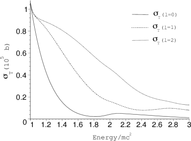
Figure 2: Behaviour of the total cross section for different values of the energy in the one delta potential case (in units of $mc^{2}$), $\sigma_{T}(l=0)$ (solid curve), $\sigma_{T}(l=1)$ (dashed curve), $\sigma_{T}(l=2)$ (dotted curve). Here we use $a=-1\hbar c$ and $r=\hbar/mc$

We first notice that those resonances in the phase shift analysis do not seem seem to have any consequences in the total cross section, in spite on their direct influence in equation (34). This has to do with the fact that the resonances in the phase shifts appear at different values of energies. The cross section vanishes smoothly for high energies. For low energies (near $mc^{2}$) the dominant channel of the angular momenta is $l=0$ (as expected). It is also important to mention that if we increase the delta radius or the coupling constant $a$ from the potential, the total cross section decreases and vanishes faster when we increase the energy.

V 2-Delta potential

Let us consider a two concentric delta potential:

$$V(r)=\pm a_{1}\delta(r-r_{1})\pm a_{2}\delta(r-r_{2}).$$ (46)

We will carry out the same procedure as before. We separate the space into three regions, finding the corresponding solution of the Dirac equation. Our potential will only affect us when $r=r_{1},r_{2}$ and, hence, the solutions are the same as for a free particle:

1) For $r<r_{1}$

$$G_{1}(r)=ra_{1}j_{l_{\kappa}}(kr),$$ (47)

$$F_{1}(r)=\frac{\kappa}{|\kappa|}\frac{k\hbar c}{E+mc^{2}}a_{1}j_{l_{-\kappa}}(kr).$$ (48)

2) For $r_{1}<r<r_{2}$

$$G_{2}(r)=r(a_{2}j_{l_{\kappa}}(kr)+b_{2}n_{l_{\kappa}}(kr)),$$ (49)

$$F_{2}(r)=\frac{\kappa}{|\kappa|}\frac{k\hbar c}{E+mc^{2}}(a_{2}j_{l_{-\kappa}}(kr)+b_{2}n_{l_{-\kappa}}(kr)).$$ (50)

3) For $r>r_{2}$

$$G_{3}(r)=r(j_{l_{\kappa}}(kr)\cos{\eta^{\pm}_{l}}-n_{l_{\kappa}}(kr)\sin{\eta^{\pm}_{l}}),$$ (51)

$$F_{3}(r)=\frac{\kappa}{|\kappa|}\frac{k\hbar c}{E+mc^{2}}(j_{l_{\kappa}}(kr)\cos{\eta^{\pm}_{l}}-n_{l_{-\kappa}}(kr)\sin{\eta^{\pm}_{l}}).$$ (52)

Using the boundary conditions for each delta and having in mind that $\alpha_{1}=\tan{(a_{1}/\hbar c)}$ and $\alpha_{2}=\tan{(a_{2}/\hbar c)}$, we can find an expression for the phase shifts:

$$\tan{\eta^{\pm}_{l}}=\frac{\alpha_{2}\left(A^{2}j^{2}_{l_{-\kappa}}+j^{2}_{l_{\kappa}}+A^{2}n_{l_{-\kappa}}j_{l_{-\kappa}}+n_{l_{\kappa}}j_{l_{\kappa}}\right)+\tilde{A}(kr_{1})\left(A(n_{l_{\kappa}}j_{l_{-\kappa}}-n_{l_{-\kappa}}j_{l_{\kappa}})\right)}{A(n_{l_{-\kappa}}j_{l_{\kappa}}-n_{l_{\kappa}}j_{l_{-\kappa}})+\alpha_{2}\left(A^{2}n_{l_{-\kappa}}j_{l_{-\kappa}}+n_{l_{\kappa}}j_{l_{\kappa}}+\tilde{A}(kr_{1})(A^{2}n^{2}_{l_{-\kappa}}+n^{2}_{l_{\kappa}})\right)},$$ (53)

where

$$A=\frac{\kappa}{|\kappa|}\frac{k\hbar c}{E+mc^{2}},$$

and

$$\tilde{A}(kr_{1})=\frac{\alpha_{1}\left(A^{2}j^{2}_{l_{-\kappa}}+j^{2}_{l_{\kappa}}\right)}{A(n_{l_{\kappa}}j_{l_{-\kappa}}-n_{l_{-\kappa}}j_{l_{\kappa}})-\alpha_{1}(n_{l_{\kappa}}j_{l_{\kappa}}+A^{2}n_{l_{-\kappa}}j_{l_{-\kappa}})}.$$ (54)

In equation (53) all Bessel functions depend only on $kr_{2}$. The dependence on $kr_{1}$ is concentrated on the function $\tilde{A}(kr_{1})$ as shown on (54). Now, if we choose $a_{1}=0$ or $r_{1}=r_{2}$ the problem, and hence the solution, reduces to a one delta potential.

Knowing the phase shifts for a two-delta potential, we can obtain an expression for the total cross section. Figure 3 shows the cross section as a function of the energy.

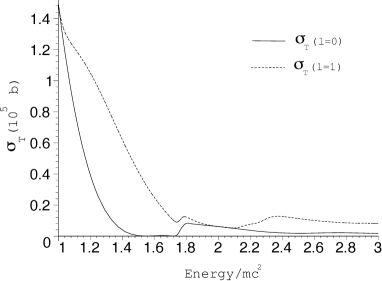
Figure 3: Behaviour of the total cross section for different values of the energy in the two delta potential case (in units of $mc^{2}$), $\sigma_{T}(l=0)$ (solid curve), $\sigma_{T}(l=1)$ (dashed curve). Here we use $a_{1}=1\hbar c$, $a_{2}=1\hbar c$, $r_{1}=2\hbar/mc$ and $r_{2}=3\hbar/mc$

Again we can see that the resonances of the phase shifts do not have any notorious influence on the total cross section, in the same way as happened for a one delta potential. It decays smoothly to zero for high energies. For small energies, near $mc^{2}$, the dominant angular momentum is the $l=0$ channel. Once again, we must remember that $l=1$ stands for the sum of $l=0,1$, and $l=2$ stands for the sum of $l=0,1,2$.

VI Born Approximation

Let us remember our potential

$$V(r)=\pm a_{1}\delta(r-r_{1})\pm a_{2}\delta(r-r_{1}).$$ (55)

Following the same steps shown in Itzykson-Zuber born (equation 2-126), we get for the scattering amplitude:

$$S_{fi}=\frac{im}{V(E_{i}E_{f})^{\frac{1}{2}}}(2\pi)\delta(E_{f}-E_{i})\int{d^{3}r\exp({-i\vec{q}\cdot\vec{r})}V(r)\bar{u}^{\alpha}(p_{f})\gamma^{0}u^{\beta}(p_{i})},$$ (56)

where $\vec{q}=\vec{p}_{f}-\vec{p}_{i}$. Then $\vec{r}\cdot\vec{r}=|\vec{q}||\vec{r}|\cos{\theta}=|\vec{q}||\vec{r}|\mu$, with $\mu=\cos{\theta}$.

Integrating in spherical coordinates: $\int^{1}_{-1}d\mu\int^{2\pi}_{0}d\phi\int^{\infty}_{0}r^{2}dr$, defining $\Gamma\equiv\bar{u}^{\alpha}(p_{f})\gamma^{0}u^{\beta}(p_{i})$, we obtain

$$S_{fi}=\frac{im}{V(E_{i}E_{f})^{\frac{1}{2}}}\frac{4\pi^{2}}{q}\delta(E_{f}-E_{i})[\pm a_{1}r_{1}\sin{qr_{1}}\pm a_{2}r_{2}\sin{qr_{2}}]\Gamma.$$ (57)

The transition probability from $i$ to $f$ per time and particle is:

$$\frac{dP_{fi}}{dt} =\int\left|\frac{im}{V(E_{i}E_{f})^{\frac{1}{2}}}\frac{2\pi}{|\vec{q}|}(\pm a_{1}r_{1}\sin{qr_{1}}\pm a_{2}r_{2}\sin{qr_{2}})\Gamma\right|^{2}$$ (58)

$$\times 2\pi\delta(E_{f}-E_{i})V\frac{d^{3}p_{f}}{(2\pi)^{3}}.$$

A straightforward calculation gives us

$$\frac{dP_{fi}}{dt}=\int\frac{m^{2}}{V(E_{i}E_{f})}\frac{(\pm a_{1}r_{1}\sin{qr_{1}}\pm a_{2}r_{2}\sin{qr_{2}})}{|\vec{q}|}|\Gamma|^{2}\delta(E_{f}-E_{i})d^{3}p_{f}.$$ (59)

To be able to find the differential cross section, we must divide the last equation by the incident flux $\frac{1}{V}\frac{|p_{i}|}{E_{i}}$

$$d\sigma=\int\frac{m^{2}}{|p_{i}|E_{f}|q|^{2}}(\pm a_{1}r_{1}\sin{qr_{1}}\pm a_{2}r_{2}\sin{qr_{2}})^{2}|\Gamma|^{2}\delta(E_{f}-E_{i})p^{2}_{f}dp_{f}d\Omega.$$ (60)

Using the fact that $|p_{i}|=|p_{f}|=p_{f}$ and $p_{f}dp_{f}=E_{f}dE_{f}$ we obtain

$$\frac{d\sigma}{d\Omega}=\frac{m^{2}}{|q|^{2}}(\pm a_{1}r_{1}\sin{qr_{1}}\pm a_{2}r_{2}\sin{qr_{2}})^{2}|\Gamma|^{2}.$$ (61)

Since we are interested in the cross section for a non polarized beam, we must sum over all $\alpha$ and $\beta$ that appear on the function $\Gamma$, this means

$$\frac{d\sigma}{d\Omega}=\frac{m^{2}}{|q|^{2}}(\pm a_{1}r_{1}\sin{qr_{1}}\pm a_{2}r_{2}\sin{qr_{2}})^{2}\sum_{\alpha}\frac{1}{2}\sum_{\beta}|\bar{u}^{\alpha}(p_{f})\gamma^{0}u^{\beta}(p_{i})|^{2}.$$ (62)

We will concentrate directly on the sum over $\alpha$ and $\beta$. Rewriting the sum as traces, we get

$$\sum_{\alpha}\frac{1}{2}\sum_{\beta}|\bar{u}^{\alpha}(p_{f})\gamma^{0}u^{\beta}(p_{i})|^{2}=\frac{1}{2}tr\left(\gamma^{0}\frac{(\gamma^{0}p_{i})+m}{2m}\gamma^{0}\frac{(\gamma^{0}p_{f})+m}{2m}\right),$$ (63)

and using some identities for the traces of the $\gamma$ matrices, we have

$$tr(\gamma^{0}(\gamma^{0}p_{i})\gamma^{0}(\gamma^{0}p_{f})=4(E_{i}E_{f}-p_{i}\cdot p_{f}+E_{i}E_{f}),$$ (64)

$$tr(\gamma^{0}\gamma^{0})=4.$$ (65)

We will also need some kinematics relations

$$E_{i}=E_{f}+E,$$ (66)

$$p_{i}\cdot p_{f}=E^{2}-p^{2}\cos{\theta}=m^{2}+2E^{2}\beta^{2}\sin^{2}{\frac{\theta}{2}},$$ (67)

where $\beta\equiv v/c=|p|/E$ is the incoming velocity. In this way we obtain

$$\frac{1}{2}tr\left(\gamma^{0}\frac{(\gamma^{0}p_{i})+m}{2m}\gamma^{0}\frac{(\gamma^{0}p_{f})+m}{2m}\right)=\frac{E^{2}}{m^{2}}(1-\beta^{2}\sin^{2}{\frac{\theta}{2}}).$$ (68)

The differential cross section with $|\vec{q}|^{2}=4|\vec{p}|^{2}\sin^{2}{\frac{\theta}{2}}=4\beta E|\vec{p}|\sin^{2}{\frac{\theta}{2}}$ is:

$$\frac{d\sigma}{d\Omega} =\frac{E(1-\beta^{2}\sin^{2}{\frac{\theta}{2}})}{4\beta|\vec{p}|\sin^{2}{\frac{\theta}{2}}}[\pm a_{1}r_{1}\sin{(2\sqrt{\beta E|\vec{p}|}\sin{\frac{\theta}{2}r_{1}})}$$ (69)

$$\pm a_{2}r_{2}\sin{(2\sqrt{\beta E|\vec{p}|}\sin{\frac{\theta}{2}r_{2}})}]^{2}.$$

We can easily see that the differential cross section is the same for attractive or repulsive potentials. One important thing to notice, when working with the partial wave method, we focus on different channels of the angular momentum. But, however, we take the sum of all the angular momenta in the Born approximation.

The total cross section is given by

$$\sigma_{total}=\int d\theta\sin{\theta}d\phi\frac{d\sigma}{d\Omega},$$ (70)

where $d\sigma/d\Omega$ is defined in (69), We obtain the following equation:

$$\sigma_{total}=\frac{2\pi E}{4\beta|\vec{p}|}\int^{\pi}_{0}d\theta\sin{\theta}[a_{1}^{2}r_{1}^{2}\sin^{2}{(\alpha_{1}\sin{\frac{\theta}{2}})}+a_{2}^{2}r_{2}^{2}\sin^{2}{(\alpha_{2}\sin{\frac{\theta}{2}})}$$

$$+2a_{1}a_{2}r_{1}r_{2}\sin{(\alpha_{1}\sin{\frac{\theta}{2}})}\sin{(\alpha_{2}\sin{\frac{\theta}{2}})}]\left(\frac{1-\beta^{2}\sin^{2}{\frac{\theta}{2}}}{\sin^{2}{\frac{\theta}{2}}}\right).$$ (71)

where $\alpha_{1}\equiv 2\sqrt{\beta E|\vec{p}}r_{1}$ y $\alpha_{2}\equiv 2\sqrt{\beta E|\vec{p}}r_{2}$. We must notice that the factor $\pm$ is not taken into account. As before we realized that there will be no influence on the results if both delta potentials are repulsive or attractive. The case where the sign of $a_{1}$ is different from the sign of $a_{2}$ will also not give new information. Integrating directly (VI) we obtain:

$$\sigma_{total} =\frac{\pi E}{2\beta|\vec{p}|}\{-2Ci(2\alpha_{1})(a_{1}r_{1})^{2}-2Ci(2\alpha_{2})(a_{2}r_{2})^{2}+2\ln{(2\alpha_{1})}(a_{1}r_{1})^{2}$$ (72)

$$+2\ln{(2\alpha_{2})}(a_{2}r_{2})^{2}-\beta^{2}((a_{1}r_{1})^{2}+(a_{2}r_{2})^{2})$$

$$+\beta^{2}\left(\frac{\sin{(2\alpha_{1})}}{\alpha_{1}})(a_{1}r_{1})^{2}+\frac{\sin{(2\alpha 2})}{\alpha_{2}}(a_{2}r_{2})^{2}\right)$$

$$-\beta^{2}\left(\frac{\sin^{2}{(\alpha_{1})}}{\alpha_{1}^{2}}(a_{1}r_{1})^{2}+\frac{\sin^{2}{(\alpha 2})}{\alpha_{2}^{2}}(a_{2}r_{2})^{2}\right)$$

$$+4(a_{1}r_{1})(a_{2}r_{2})(Ci(\alpha_{1}-\alpha_{2})-Ci(\alpha_{1}+\alpha_{2})$$

$$-\beta^{2}[\frac{\sin{(\alpha_{1}-\alpha_{2})}}{\alpha_{1}-\alpha_{2})}+\frac{\cos{(\alpha_{1}-\alpha_{2})}}{(\alpha_{1}-\alpha_{2})^{2}}-\frac{1}{(\alpha_{1}-\alpha_{2})^{2}}$$

$$-\frac{\sin{(\alpha_{1}+\alpha_{2})}}{(\alpha_{1}+\alpha_{2})}-\frac{\cos{(\alpha_{1}+\alpha_{2})}}{(\alpha_{1}+\alpha_{2})^{2}}+\frac{1}{(\alpha_{1}+\alpha_{2})^{2}}])$$

$$-C(2(a_{1}r_{1})^{2}+2(a_{2}r_{2})^{2}),$$

where $Ci$ is the well known cosine integral, given by the following equation:

$$Ci(x)=C+\ln{(x)}+\sum^{\infty}_{k=1}(-1)^{k}\frac{x^{2k}}{2k(2k)!},$$ (73)

and C is the Euler constant.

Figure 4 shows the dependence of the total cross section while we vary the energy of the particles. We notice that the total cross section has the same behavior found in the partial wave method. On the other hand if we take a $\Delta r=r_{2}-r_{1}=cte$, we can see that the behavior is again similar to the one we found in the partial wave method.

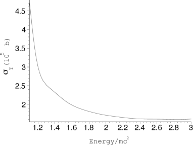
Figure 4: Behaviour of the total cross section for different values of the energy in the two delta potential case (in units of $mc^{2}$) with the Born Approximation. Here we use $a_{1}=-1\hbar c$, $a_{2}=-1\hbar c$, $r_{1}=2\hbar/mc$ and $r_{2}=3\hbar/mc$

We can say that the behavior of the cross section given by the sum of all the angular momenta is similar to the behavior of the cross section for a specific angular momentum channel. In spite of several efforts, we were unable to find geometric conditions related to the separation of the two delta potentials, and the possible occurrence of resonances as peaks in the total cross section.

VII Conclusions

The general idea of this work was to use the boundary conditions obtained in loewe , when working with delta type singular potentials, in particular for a spherical potential like $V(r)=\pm a\delta(r-r_{0})$ in the scattering region. We studied the behavior of the phase shifts, the differential and total cross section.

We found a direct relation between the phase shifts of the scattered wave and the cross section. With this we were able to calculate values of the cross section for different angular momentum channels, giving us valuable information, in particular, the dependence of the cross section on the $l=0$ channel in the low energy limit.

It is important to notice that the behavior of the cross sections for each channel of the angular momenta is very similar for repulsive and attractive potentials, in the one and two delta cases. We confirmed our results through the calculation of the cross section within the Born approximation. This method does not require the knowledge of the boundary conditions, but it does not give us information about the angular momenta of the particles.

It could be interesting to expand this work to an anion-potential, i.e. a series of concentric delta-potentials, trying to find recurrence relations for the occurrence of resonances in the different angular momentum channels.

References

• (1) C. Cohen-Tannoudji, B. Diu and F. Lalo$\ddot{e}$. Quantum Mechanics 1977 (New York: Wiley).
• (2) R. Benguria,H. Castillo and M. Loewe, J. Phys. A: Math Gen. 33 (2000) 5315.
• (3) J. Dittrich, P. Exner and P. S̆eba J. Math. Phys. 30 (1989) 2875, and J. Math. Phys. 33 (1992) 2207.
• (4) W. Greiner, B. Müller, and J. Rafelski, Quantum Electrodynamics of Strong Fields 1985 (Berlin: Springer).
• (5) M. E. Rose, Relativistic Electron Theory 1961 (New York: Wiley).
• (6) M. Dapor, Quantum Electron-Atom Scattering: An Introduction 1999 (New York: Nova Science Publishers, Inc).
• (7) A. Gray and G. B. Mathews, A Treatise on Bessel Functions and Their Applications to Physics 1966 (New York: Dover).
• (8) C. Itzykson, J. B. Zuber, Quantum Field Theory 1980 (New York: McGraw Hill).