External Time-Varying Fields and Electron Coherence

Abstract

The effect of time-varying electromagnetic fields on electron coherence is investigated. A sinusoidal electromagnetic field produces a time varying Aharonov-Bohm phase. In a measurement of the interference pattern which averages over this phase, the effect is a loss of contrast. This is effectively a form of decoherence. We calculate the magnitude of this effect for various electromagnetic field configurations. The result seems to be sufficiently large to be observable.

The well-known Aharonov-Bohm phase AB1959 arises when coherent electrons traverse two distinct paths in the presence of an electromagnetic field. Let the two paths in spacetime be denoted by $C_{1}$ and $C_{2}$. The phase difference due to the electromagnetic field, the Aharonov-Bohm phase, is the line integral of the vector potential around the closed spacetime path $\partial\Omega=C_{1}-C_{2}$:

$$\vartheta=-e\oint_{\partial\Omega}dx_{\mu}A^{\mu}(x)\,.$$ (1)

By Stoke’s theorem, it can also be expressed as a surface integral of the field strength tensor over a two dimensional surface $\Omega$ bounded by $\partial\Omega$:

$$\vartheta=-\frac{1}{2}e\int_{\Omega}d\sigma_{\mu\nu}\,F^{\mu\nu}(x)\,.$$ (2)

This leads to the remarkable result that the electron interference pattern is sensitive to shifts in the field strength in regions from which the electrons are excluded. The reality of the Aharonov-Bohm effect has been confirmed by numerous experiments, beginning with the work of Chambers rC1960 and continuing with that of Tonomura and coworkers aT1982 using electron holography.

If the electromagnetic field undergoes fluctuations on a time scale shorter than the integration time of the experiment, then the effect is a loss of contrast in the interference pattern. The role of a fluctuating Aharonov-Bohm phase in decoherence has been discussed by several authors SAI1990 ; lF1993 ; lF1995 ; lF1997 ; BP2001 ; BP2000 ; MPV2003 . The amplitude of the interference oscillations is reduced by a factor of

$$\Upsilon=\left\langle{\rm e}^{i\vartheta}\right\rangle\,,$$ (3)

where the angular brackets can denote either an ensemble or a time average. In the case of Gaussian or quantum fluctuations with $\langle\vartheta\rangle=0$, this factor becomes

$$\Upsilon={\rm e}^{-\frac{1}{2}\langle\vartheta^{2}\rangle}\,.$$ (4)

This form also holds in the case of thermal fluctuations BP2001 .

In our treatment, we assume an approximation in which the electrons move on classical trajectories. More generally, the electrons are in wavepacket states. However, under many circumstances, the sizes of the wavepackets can be small compared to the path separation, so the classical path approximation is good. Wavepacket sizes which have been realized in experiments NH93 can be less than $1\,{\rm\mu m}$, which is one to two orders of magnitude smaller than the other length scales characterizing the paths. A more detailed discussion of the effects of finite wavepacket size was given in Ref. lF1997 .

The purpose of the present paper is to discuss a particularly simple version of this type of decoherence produced by a classical, sinusoidal electromagnetic field. If the period of oscillation of the field is short compared to the time scale over which the interference pattern can be measured, then a time average must be taken in Eq. (3), with a resulting loss of contrast.

We consider the case of a linearly polarized, monochromatic electromagnetic wave of frequency $\omega$ which propagates in a direction perpendicular to the plane containing the electron beams. Let the wave be polarized in the $z$-direction and propagate in the $y$-direction, with the plane of the electron paths being the $x$-$z$ plane. For a path confined to this plane, we have

$$\frac{1}{2}\,d\sigma_{\mu\nu}\,F^{\mu\nu}=dt\,dx\,F^{tx}+dt\,dz\,F^{tz}+dx\,dz\,F^{xz}\,.$$ (5)

In the present case, where $E^{x}=B^{y}=0$, Eq. (2) becomes

$$\vartheta=e\int dt\,dz\,E^{z}\,.$$ (6)

Let the $z$-component of the electric field take the form

$$E^{z}(x^{\mu})=\mathbb{E}(x,y,z)\cos(k\,y-\omega\,t),$$ (7)

where the real modulated amplitude $\mathbb{E}(x,y,z)$ is assumed to be a slowly varying function of $y$, compared with the sinusoidal oscillation. We can write

$$\vartheta(t_{0})=e\!\int_{\Omega}dt\,dz\,\mathbb{E}(x,y,z)\cos(k\,y-\omega\,t-\omega\,t_{0})\,,$$ (8)

where $t_{0}$ is the electron emission time. More precisely, it is the time at which the center of a localized wavepacket is emitted. If the measuring process takes a sufficiently long time compared with the electron flight time, we will observe a result which is averaged over $t_{0}$. Therefore, let $t_{0}$ be a random variable and take the time average over that variable. That is, for a function $f$ of a random time variable $\xi$, the time average is defined by

$$\bigl{<}f(\xi)\bigr{>}\equiv\lim_{\Xi\rightarrow\infty}\frac{1}{2\,\Xi}\int_{-\Xi}^{+\Xi}d\xi\,f(\xi).$$ (9)

However, before taking the time average, we will rewrite Eq. (8) as

$$\vartheta=\mathbb{A}\cos(\omega\,t_{0})+\mathbb{B}\sin(\omega\,t_{0}),$$ (10)

where

$$\mathbb{A}=e\!\int_{\Omega}dt\,dz\,\mathbb{E}(x,y,z)\cos(k\,y-\omega\,t),$$ (11)

$$\mathbb{B}=e\!\int_{\Omega}dt\,dz\,\mathbb{E}(x,y,z)\sin(k\,y-\omega\,t),$$ (12)

and we have the average of the time-varying phase factor given by,

$$\Upsilon=\bigl{<}e^{i\vartheta}\bigr{>} =\lim_{\Xi\rightarrow\infty}\frac{1}{2\,\Xi}\!\int_{-\Xi}^{+\Xi}\!dt_{0}\;e^{i\,\bigl{[}\mathbb{A}\cos(\omega\,t_{0})+\mathbb{B}\sin(\omega\,t_{0})\bigr{]}},$$

$$=J_{0}\bigl{(}\left|\,\mathbb{C}\,\right|\bigr{)},$$ (13)

where $J_{0}$ is a Bessel function and

$$\mathbb{C} =\mathbb{A}+i\,\mathbb{B}$$

$$=e\!\int_{\Omega}dt\,dz\,\mathbb{E}(x,y,z)\,e^{i(k\,y-\omega\,t)}.$$ (14)

Note that in the limit that $|\mathbb{C}|\ll 1$, we can Taylor expand the Bessel function $J_{0}$ and write

$$\Upsilon\approx 1-\frac{1}{4}|\mathbb{C}|^{2}+\frac{1}{64}|\mathbb{C}|^{4}+\cdots\,.$$ (15)

This agrees through order $|\mathbb{C}|^{2}$ with the result that would be obtained from Eq. (4) for Gaussian fluctuations, as $\langle\vartheta^{2}\rangle=\frac{1}{2}|\mathbb{C}|^{2}$.

As the strength of the applied field increases, the contrast factor $\Upsilon$ will monotonically decrease until the first zero of $J_{0}$ at $|\mathbb{C}|=2.405$ is reached. Beyond that point, the contrast will begin to increase and then undergo damped oscillations. This behavior is quite different from that produced by Gaussian fluctuations, Eq. (4).

Now we study the possible effect on the electron interference if we shine a non-localized beam over the electron paths. Because the plane wave extends to infinity in the transverse direction, it is inevitable that the electron will have direct interaction with the electromagnetic fields, However, it will be shown later that the direct interaction with the electromagnetic fields is extremely small, so it can be ignored. Some years ago, Dawson and Fried DF1967 discussed the effect of a laser beam on coherent electrons. However, these authors were concerned with a change in phase, rather than the loss of contrast with which we are concerned.

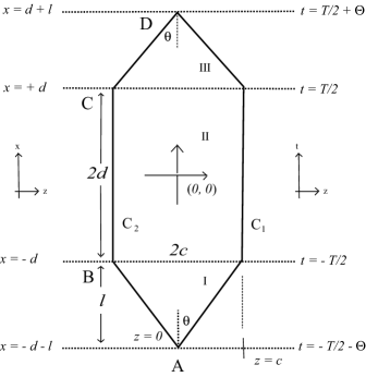
Figure 1: The two possible electron paths, $C_{1}$ and $C_{2}$ are illustrated. The electrons start at point $A$ and end at point $D$ after traversing a path which is approximated by three straight line segments. Here $\Theta$ is the time required for the first and last segments, and $T$ is the time required for the middle segment.

Assume that the transverse plane wave of amplitude $\mathcal{E}_{0}$ propagates along the $y$ axis and is polarized in the $z$ direction. The electron paths lie on the $y=0$ plane and are illustrated in Fig. 1. The quantity $\mathbb{C}$ is then given by

$$\mathbb{C}=4\,e\,\mathcal{E}_{0}\biggl{(}\frac{2c}{\omega^{2}\Theta}\biggr{)}\sin\biggl{[}\frac{\omega\,\Theta}{2}\biggr{]}\sin\biggl{[}\frac{1}{2}\,\omega\left(T+\Theta\right)\biggr{]}.$$ (16)

Here $2c$ is the maximum separation between the elctron paths. Experimentally attainable separations are of the order of $100\,\mu m$ Hasselbach .

The quantity $\left|\,\mathbb{C}\,\right|^{2}$ is written as

$$\left|\,\mathbb{C}\,\right|^{2} =16\,e^{2}\mathcal{E}_{0}^{2}\biggl{(}\frac{2c}{\omega^{2}\Theta}\biggr{)}^{2}\sin^{2}\biggl{[}\frac{\omega\,\Theta}{2}\biggr{]}\sin^{2}\biggl{[}\frac{1}{2}\,\omega\left(T+\Theta\right)\biggr{]}$$

$$\approx\frac{32\pi}{137}\,\rho\,\biggl{(}\frac{2c}{\omega^{2}\Theta}\biggr{)}^{2}\,,$$ (17)

where the squares of the sine functions have been replaced by their average value of $1/2$ and the averaged energy density $\rho$ is given by

$$\rho=\frac{1}{2}\,\mathcal{E}_{0}^{2}.$$ (18)

We use Lorentz-Heaviside units with $\hbar$ and the speed of light set equal to unity. Thus, $\rho$ is also the energy flux in the electromagnetic wave. Note that $\Theta=s/v$, where $v$ is the electron’s speed and $s=\sqrt{c^{2}+l^{2}}$ is the length of the first and third segments of the paths. If the electron’s speed is nonrelativistic, we can write

$$\left|\,\mathbb{C}\,\right|^{2}=\left(\frac{E_{k}}{5\,{\rm keV}}\right)\left(\frac{\rho}{1\,{\rm W/cm}^{2}}\right)\left(\frac{2c}{s}\right)^{2}\left(\frac{\lambda}{100\,\mu{\rm m}}\right)^{4}\,,$$ (19)

where $E_{k}$ is the electron kinetic energy and $\lambda$ is the wavelength of the electromagnetic wave. Thus it seems plausible that one could arrange to have $\left|\,\mathbb{C}\,\right|^{2}$ large enough to produce experimentally observable effects.

There are some comments on this calculation: First, we assumed electron paths with sharp corners for simplicity. If one were to round out the corners slightly to make more realistic paths, the result need not change significantly. This is because we are integrating a regular integrand which varies on a time scale of the order of $1/\omega$. If the actual time scale for the electron to change direction is small compared to this time, then our piecewise trajectory is a good approximation. Note that here we are discussing the change in contrast due to the applied field. Sharp corners will tend to cause emission of photons, which in turn lead to decoherence even in the absence of an applied field. A second comment is that the contributions of each of the three regions, I, II and III, in Fig. 1 is large compared to the final result for $\mathbb{C}$ by a factor of the order of $\Theta\,\omega$. However, the leading terms cancel when the three contributions are summed, leading to Eq. (External Time-Varying Fields and Electron Coherence). Finally, we have assumed that the electron paths are localized, whereas in an actual experiment the classical trajectories will be replaced by bundles of finite thickness. What is required here is that the electron beams be localized in the $y$-direction on a scale small compared to the wavelength of the electromagnetic field.

Since the electron passes through the region where the electromagnetic fields are non-zero, it has a direct interaction with the fields. Due to the fact that the electron is in non-relativistic motion, in the low energy limit, only Thomson scattering is considered. Let $n$ be the mean number density of photons, which can approximately be expressed in terms the electromagnetic energy density $\rho$ and the angular frequency $\omega$ as

$$n\simeq\frac{\rho}{\omega},$$ (20)

for very large $n$. As a result, the mean free path $l_{\rm mfp}$ of the Thomson scattering is given by

$$l_{\rm mfp} =\frac{1}{n\,\sigma_{T}}=\frac{\omega}{\sigma_{T}\,\rho}$$ (21)

$$=9\times 10^{13}\textit{m}\,\Bigl{(}\frac{\rho}{{\rm W/cm}^{2}}\Bigr{)}^{-1}\Bigl{(}\frac{\lambda}{\mu{\rm m}}\Bigr{)}^{-1}\,,$$ (22)

where $\sigma_{T}$ is the Thomson cross section. We can see that it is possible to have an incident flux which is large enough to produce observable decoherence but for which any effect from the electron-photon scattering may be ignored. That is, loss of phase coherence due to direct electron-photon scattering arises from the random accumulated electron wavefunction phase shifts from one or more such scattering events. However, in many realistic situations, the probability of even one such event per electron is close to zero.

The above analysis shows that the change of contrast is really due to a variant of the Aharonov-Bohm effect, the averaging over the time-dependent Aharonov-Bohm phase created by fields in the interior of the electron path. It is not due to direct scattering between electrons and photons. Nonetheless, it is also of interest to consider a configuration where the applied electromagnetic field is localized in a region between the electron paths. An example is a Gaussian beam. Let the electric field in the plane of the paths be given by

$$E^{z}({\bf\rho})=\mathcal{E}_{0}\,\exp\left(-\frac{{\boldsymbol{\rho}}^{2}}{\sigma^{2}}\right)\,\cos(\omega\,t)\,,$$ (23)

where $\boldsymbol{\rho}$ is the radius vector in the plane and $\sigma$ is the effective width of the beam in this plane. This form is a good approximation to the electric field of a linearly polarized laser beam. Suppose that this beam is normally incident upon the electron paths illustrated in Fig. 1, with the center of the beam being at the origin in this figure. A calculation which will be presented in detail in Ref. HF2004 leads to the result, for the case that $\sigma\lesssim 2c$ and $\sigma\lesssim 2d$,

$$\mathbb{C}\approx-\frac{8\sqrt{\pi}e\mathcal{E}_{0}d^{2}}{\omega^{2}T\sigma}\,(1-\cos\theta)\,\cos\left(\frac{\omega T}{2}\right)\,\exp\left(-\frac{d^{2}}{\sigma^{2}}\right)\,.$$ (24)

The crucial feature of this result is the factor of $\exp(-d^{2}/\sigma^{2})$, which is extremely small in the limit of a highly localized beam, $\sigma\ll d$.

To summarize, in this paper we have investigated the effects of a rapidly varying Aharonov-Bohm phase upon an electron interference pattern. If the time scale for the variation is short compared to the time during which the pattern is measured, then averaging over the phase variations leads to a loss of contrast. This is a form of decoherence. In principle, the lost contrast could be restored if one were able to select only those electrons which start at a fixed point in the cycle of an oscillatory Aharonov-Bohm phase. The form of decoherence studied here is an example of zero temperature decoherence. Other forms of zero temperature decoherence, which do not rely upon thermal effects, have been discussed in Refs. Sinha97 ; WMJ98 ; WG01 .

We have calculated the size of the decoherence effect produced by a monochromatic, linearly polarized electromagnetic field. The result seems to be large enough to be observable. We primarily treated the case of a non-localized plane wave. In this case, although the electromagnetic field is nonzero at the location of the electrons, we argued that one can have an observable loss of contrast even when the probability of an electron scattering from a photon is extremely small. A unique signature of the decoherence produced by sinusoidal fields is that the interference pattern can disappear and then reappear as the field strength is increased.

- (1) Y. Aharonov and D. Bohm, Phys. Rev. 115, 485 (1959).
- (2) R.G. Chambers, Phys. Rev. Lett. 5, 3 (1960).
- (3) A. Tonomura, et al, Phys. Rev. Lett. 48, 1443 (1982).
- (4) A. Stern, Y. Aharonov, and Y. Imry, Phys. Rev. A 41, 3436 (1990).
- (5) L.H. Ford, Phys. Rev. D 47, 5571 (1993).
- (6) L.H. Ford, Ann. NY. Acad. Sci. 755, 741 (1995).
- (7) L.H. Ford, Phys. Rev. A 56, 1812 (1997).
- (8) H.P. Breuer and F. Petruccione, Phys. Rev. A 63, 032102 (2001).
- (9) H.P. Breuer and F. Petruccione, in Relativistic Quantum Measurement and Decoherence, edited by H.P. Breuer and F. Petruccione (Springer-Verlag, Berlin, 2000).
- (10) F.D. Mazzitelli, J.P. Paz, and A. Villanueva, Phys. Rev. A 68, 062106 (2003).
- (11) M. Nicklaus and F. Hasselbach, Phys. Rev. A 48, 152 (1993).
- (12) J.F. Dawson and Z. Fried, Phys. Rev. Lett. 19 467 (1967).
- (13) F. Hasselbach, Z. Phys. B 71, 443 (1988).
- (14) J-T. Hsiang and L.H. Ford, to be published.
- (15) S. Sinha, Phys. Lett. A 228, 1 (1997).
- (16) R.A. Webb, P. Mohanty, and E.M.Q. Jariwala, Fortsch. Phys. 46 779 (1998).
- (17) V. Wong and M. Gruebele, Phys. Rev. A 63, 022502 (2001).