Exciton entanglement in two coupled semiconductor microcrystallites

Abstract

Entanglement of the excitonic states in the system of two coupled semiconductor microcrystallites, whose sizes are much larger than the Bohr radius of exciton in bulk semiconductor but smaller than the relevant optical wavelength, is quantified in terms of the entropy of entanglement. It is observed that the nonlinear interaction between excitons increases the maximum values of the entropy of the entanglement more than that of the linear coupling model. Therefore, a system of two coupled microcrystallites can be used as a good source of entanglement with fixed exciton number. The relationship between the entropy of the entanglement and the population imbalance of two microcrystallites is numerically shown and the uppermost envelope function for them is estimated by applying the Jaynes principle.

published in J. Phys. A 37, 4423-4436 (March 2004)

PACS numbers 03.67.-a, 71.10.Li, 71.35.-y, 73.20Dx

1 Introduction

Recently, quantum computation and quantum information excite large enthusiasm among theoretical and experimental physicists. Many theoretical and experimental researches have been devoted to the preparation and measurement of the entangled states that have been considered to be a key ingredient in the realization of the quantum computation and information.

We can quantitatively understand the role of quantum entanglement as a resource for communication by studying the quantum teleportation, which was first realized for discrete variables [1] and then for continuous variables [2]. The possibility for the generation of the maximally entangled states with a fixed photon number from squeezed vacuum states or from mixed Gaussian continuous entangled states by the quantum non-demolition measurement [3] has been theoretically studied. Quantum teleportation using an entangled source of fixed total photon number has also been theoretically investigated in [5]. However, it has been shown that a generation of the maximally entangled states with a fixed finite photon number is a great challenge to modern technology. So the exploration of new maximally entangled bipartite source with fixed particle number is very interesting and important from both experimental and theoretical view points.

Several schemes based on coupled quantum dots have been proposed for fabricating quantum gates [6, 9]. The entanglement of the exciton states in a single quantum dot or in a quantum dot molecule has been demonstrated experimentally [10, 11]. The authors of references [12, 14, 15, 16] theoretically investigated the entanglement of excitonic states in the system of the optically driven coupled quantum dots and propose models to prepare Bell, Greenberger-Horne-Zeilinger (GHZ) and $W$ states. The above investigations mainly focus on the case in which the sizes of quantum dots are smaller than the Bohr radius of exciton in bulk semiconductor, so that the quantum dots have discrete energy levels and one energy state can only be occupied by one exciton because of the Pauli principle. In such quantum dot systems, it is easy to define a qubit by different spins of excitons, or by single-exciton and no-exciton states. So when we want to encode quantum information in systems of quantum dots by a finite-dimensional quantum state space (called qudit system), we need to consider higher energy levels. However, if we can enlarge the size $R$ of the quantum dot so that it is larger than the Bohr radius $a_{B}$ of the exciton in the bulk semiconductor but smaller than the relevant light wavelength $\lambda$, in such a system of quantum microcrystallites (which can also be called large quantum dots system [20, 21, 23]), the excitons can occupy the same level when the average number of excitons per Bohr radius volume is less than one. Then we can encode quantum information in the finite Hilbert space built by the different exciton number states. Quantum information properties of semiconductor microcrystallites coupled by a cavity field were investigated by us in Refs. [24] where, in particular, we have proposed a realization of symmetric sharing of entanglement for the exciton states in semiconductor microcrystallites and also studied the environment effect on the qubit.

Motivated by these considerations, in this paper we will study a system of two semiconductor microcrystallites coupled by Coulomb interaction. We will study the entanglement of the qudit excitonic states in these two coupled semiconductor microcrystallites with fixed exciton number.

The paper is organized as follows: In Sec. II, we first give a theoretical description of two coupled semiconductor microcrystallites. We obtain the analytical solution of the system by virtue of the Schwinger representation of the angular momentum. In Sec. III, the entanglement of the two subsystems is discussed using the von Neumann entropy under certain initial conditions. We discuss and numerically analyze the oscillation of the exciton population imbalance between two quantum dots. The relationship between the entanglement and oscillation of the imbalance population of excitons is demonstrated in detail in Sec. IV. Finally, we give our conclusions and some comments.

2 The model and its analytical solution

We consider a system which consists of two semiconductor microcrystallites coupled by Coulomb interaction. We assume that two semiconductor microcrystallites are completely symmetric. Their sizes are larger than the Bohr radius $a_{B}$ of an exciton in a bulk semiconductor but smaller than the relevant light wavelength $\lambda$. Using two-band approximation to model these two coupled semiconductor microcrystallites, we have the Hamiltonian

$$H=\hbar\sum_{j,k=1}^{2}\chi_{jk}a^{\dagger}_{j}a_{k}+\sum_{j,k,l,m=1}^{2}\chi_{jklm}a^{\dagger}_{j}a^{\dagger}_{k}a_{l}a_{m},$$ (1)

where $a^{\dagger}_{j}\,(a_{j})$ are creation (annihilation) operators of excitons, which are electron-hole pairs bound by the Coulomb interaction. We assume that the density of the excitons is so low and the external confinement potential to microcrystallite is so weak that the exciton operators $a^{\dagger}_{j}\,(a_{j})$ can be described approximately as bosonic operators, that is they satisfy the commutation relations of the ideal bosons, $[a_{j},a^{\dagger}_{k}]=\delta_{jk}$, which is somewhat different from that in Ref. [27]. The label $j$=1 (2) denotes the microcrystallite $A\,(B)$. In the Hamiltonian (1), the deviation of the exciton operators from the ideal bosonic model is corrected by introducing an effective nonlinear interaction between the hypothetical ideal bosons. In general, the parameters $\chi_{jk}$ are different from each other, however in this study we consider two completely equivalent microcrystallites, which have nearly the same Bohr radius of the excitons and transitional dipole moment. For the sake of simplicity, we assume the parameters $\chi_{jk}=\omega>0$ for $j=k$, which means that the two semiconductor microcrystallites have the same transition frequency from the valence band to the conduction band, and assume positive real numbers $\chi_{jk}=g$ for $j\neq k$, which correspond to a linear coupling constant of the two semiconductor microcrystallites. The parameters $\chi_{jklm}$ of the nonlinear terms are also taken as positive constant and set to be $\chi_{jklm}=\chi$. Under these assumptions, the Hamiltonian (1) can be simplified as follows

$$H = \hbar\Omega{\bf N}+\hbar\chi{\bf N}^{2}+\hbar{\bf G}(a^{\dagger}_{1}a_{2}+a^{\dagger}_{2}a_{1})$$ (2)

$$+\hbar\chi(a^{\dagger}_{1}a_{2}+a^{\dagger}_{2}a_{1})^{2},$$

where $\Omega=\omega-2\chi$, and ${\bf G}=g-2\chi+2\chi{\bf N}$. It is obvious that ${\bf N}=a^{\dagger}_{1}a_{1}+a^{\dagger}_{2}a_{2}$ is a constant of motion, which means $[{\bf N},H]=0$ and the total exciton number of the coupled semiconductor microcrystallites is conserved. In such a situation, we find that it is more convenient to get the solution of the Schrödinger equation governed by Hamiltonian (2) by virtue of Schwinger representation of the angular momentum [28, 29]. That is, we can introduce the angular momentum operators

$$J_{x} = \frac{1}{2}(a^{\dagger}_{1}a_{2}+a^{\dagger}_{2}a_{1}),$$ (3a)

$$J_{y} = \frac{1}{2i}(a^{\dagger}_{1}a_{2}-a^{\dagger}_{2}a_{1}),$$ (3b)

$$J_{z} = \frac{1}{2}(a^{\dagger}_{1}a_{1}-a^{\dagger}_{2}a_{2})$$ (3c)

from the bosonic annihilation and creation operators of the two exciton modes. The operators of (3a)–(3c) satisfy the commutation relations for the Lie algebra of SU(2):

$$[J_{j},J_{k}]=i\varepsilon_{jkl}J_{l},\hskip 14.22636ptj,k,l=x,y,z,$$ (4)

where the Levi-Cività tensor $\varepsilon_{jkl}$ is equal to $+1$ and $-1$ for the even and the odd permutation of its indices, respectively, and zero otherwise. From (3a)–(3c), the total angular momentum operator can be expressed as

$$J^{2}=\frac{\bf N}{2}(\frac{\bf N}{2}+1).$$ (5)

In fact, ${\bf N}$ itself commutes with all the operators (3a)–(3c) and (5). For a fixed total excitonic number $\cal{N}$, the common eigenstates of $J^{2}$ and $J_{z}$ are the two-mode Fock states [28, 29]

$$|j,m\rangle_{s}=|m_{1},m_{2}\rangle=\frac{(a_{1}^{\dagger})^{j+m}(a_{2}^{\dagger})^{j-m}}{\sqrt{(j+m)!(j-m)!}}|0\rangle$$ (6)

with eigenvalues $j={\cal N}/2$ and $m=-{\cal N}/2,\cdots,{\cal N}/2$, where $|m_{1},m_{2}\rangle$ is the Fock state with $m_{1}=j+m$ excitons and $m_{2}=j-m$ excitons in microcrystallite $A$ and microcrystallite $B$ respectively. Although $j\pm m$ $(m_{1},m_{2})$ must be integers, $j$ and $m$ can both be integers or half-odd integers. For consistency, $j$ is replaced by ${\cal N}/2$ in the following expressions. For clarity, the subscript $s$ is used to indicate the Schwinger angular momentum basis in (6) and the following equations. By using equation (6), we take $j=1$ and $m=0$ as a detailed example to show the relation between the Schwinger angular momentum basis and Fock state basis. That is, $|1,0\rangle_{s}=a_{1}^{\dagger}a_{2}^{\dagger}|0\rangle=|1,1\rangle$ which means that when the quantum number of the total angular momentum $j$ is $1$ and its $z$ component $m$ is $0$, there is one exciton in each microcrystallite respectively.

In terms of an ${\rm SO(3)}$ rotation $e^{i{\pi}/{2}J_{y}}$ of $2\hbar{\bf G}J_{x}+4\hbar\chi J_{x}^{2}$, equation (2) can be simplified into :

$$H = \hbar\Omega{\bf N}+\hbar\chi{\bf N}^{2}+2\hbar{\bf G}J_{x}+4\hbar\chi J_{x}^{2}$$ (7)

$$= \hbar\Omega{\bf N}+\hbar\chi{\bf N}^{2}+2\hbar{\bf G}e^{-i({\pi}/{2})J_{y}}J_{z}e^{i({\pi}/{2})J_{y}}$$

$$+4\hbar\chi e^{-i({\pi}/{2})J_{y}}J_{z}^{2}e^{i({\pi}/{2})J_{y}}.$$

The eigenfunctions $\Psi_{{\cal N}/2,m}$ and the eigenvalues $E_{{\cal N}/2,m}$ of Hamiltonian (7) can be obtained easily as

$$|\Psi_{\frac{\cal N}{2},m}\rangle_{s} = e^{(-i\pi/2)J_{y}}|\frac{\cal N}{2},m\rangle_{s}=\sum_{m^{\prime}=-\frac{\cal N}{2}}^{\frac{\cal N}{2}}{\cal D}^{\frac{\cal N}{2}}_{m^{\prime}m}({\textstyle\frac{\pi}{2}})|\frac{\cal N}{2},m^{\prime}\rangle_{s},$$ (8a)

$$E_{{\cal N}/2,m} = \hbar\Omega{\cal N}+\hbar\chi{\cal N}^{2}+2\hbar{\cal G}m+4\hbar\chi m^{2},$$ (8b)

where ${\cal N}$ denotes the total excitonic number of two microcrystallites; ${\cal G}=g-2\chi+2\chi{\cal N}$, and Wigner’s formula for ${\cal D}^{\frac{\cal N}{2}}_{m^{\prime}m}(\frac{\pi}{2})$ reads as

$${\cal D}^{\frac{\cal N}{2}}_{m^{\prime}m}(\frac{\pi}{2}) = \sum_{k}(-1)^{k-m-m^{\prime}}(\textstyle\frac{1}{2})^{\frac{\cal N}{2}}$$ (9)

$$\times\frac{\sqrt{(\frac{\cal N}{2}+m)!(\frac{\cal N}{2}-m)!(\frac{\cal N}{2}+m^{\prime})!(\frac{\cal N}{2}-m^{\prime})!}}{(\frac{\cal N}{2}+m-k)!k!(\frac{\cal N}{2}-k-m^{\prime})!(k-m+m^{\prime})!},$$

where we take the sum over $k$ so that none of the arguments of factorials in the denominator is negative. The wave function $|\Psi(t)\rangle$ of the system for the initial condition $|\Psi(t=0)\rangle$ is given by

$$|\Psi(t)\rangle = \exp(-itH/\hbar)|\Psi(0)\rangle=\sum_{{\cal N}=0}^{\infty}\sum_{m=-{\cal N}/2}^{m={\cal N}/2}$$ (10)

$$\times\exp\left(\frac{E_{\frac{\cal N}{2},m}}{i\hbar}t\right)\langle\Psi_{\frac{\cal N}{2},m}|\Psi(0)\rangle|\Psi_{\frac{\cal N}{2},m}\rangle_{s}.$$

The coefficients $\langle\Psi_{\frac{N}{2},m}|\Psi(0)\rangle$ are rotating matrix elements that can be determined by Wigner’s formula. Equation (10) is basic and will be used in our further discussions. In the following two sections, we will discuss the entanglement of two exciton modes and demonstrate the oscillations of population imbalance for excitons between two quantum microcrystallites.

3 Entanglement of the excitonic states

Quantum entanglement plays the key role in the quantum information and quantum computation. In general, for any pure composite state $|\psi\rangle_{AB}$ of a bipartite system whose state space is $H_{A}\otimes H_{B}$, the entanglement can be measured by von Neumann’s entropy of any reduced density operator $\rho_{A}={\rm Tr}_{B}(|\psi\rangle\!_{AB}\,{}_{AB}\!\langle\psi|)$ or $\rho_{B}={\rm Tr}_{A}(|\psi\rangle\!_{AB}\,{}_{AB}\!\langle\psi|)$, where the reduced density operator of system $A$ is obtained by tracing out system $B$ and that of system $B$ by tracing out system $A$. In the context of quantum computation and information, in particular in studies of quantum entanglement, the reduced von Neumann entropy of a bipartite pure state $|\psi\rangle_{AB}$ is usually referred to as the entropy of entanglement or simply the entanglement (see, e.g., [30, 31, 32, 33]):

$$E(\rho) = -{\rm Tr}(\rho_{A}\ln\rho_{A})=-{\rm Tr}(\rho_{B}\ln\rho_{B})=-\sum_{n}\lambda_{n}\ln\lambda_{n}$$ (11)

where $\lambda_{n}$ are the eigenvalues of either $\rho_{A}$ or $\rho_{B}$. They form the (square of the) coefficients of the Schmidt decomposition of the bipartite pure state. That is, the bipartite pure state $|\psi\rangle_{AB}$ can be expressed by a set of biorthogonal vectors using the Schmidt decomposition as

$$|\psi\rangle\equiv|\psi\rangle_{AB}=\sum_{n}\sqrt{\lambda_{n}}|\alpha_{n}\rangle_{A}|\beta_{n}\rangle_{B}$$ (12)

where we have chosen the phases of our basis states so that no phases appear in the coefficients $\lambda_{n}$ in the sum of (12), $\{|\alpha_{n}\rangle,n=0\cdots\}$ and $\{|\beta_{n}\rangle,n=0\cdots\}$ are orthonormal states of the two subsystems $A$ and $B$ respectively.

The total number of excitons in the whole system is fixed by the initial condition, such as $L$. Based on such a condition, the maximally entangled state of the system is

$$|M\rangle=\frac{1}{\sqrt{L+1}}\sum_{l=0}^{L}|L-l,l\rangle,$$ (13)

where $|L-l,l\rangle$ represents the state with $L-l$ excitons in microcrystallite $A$ and $l$ excitons in microcrystallite $B$. According to definition (11), the entropy of the entanglement for the maximally entangled state (13) is $\ln(1+L)$.

Experimentally, the easier way is to excite some number of excitons in one microcrystallite, or both of microcrystallites. Without loss of generality, we first assume that microcrystallite $A$ is initially excited with $L$ excitons, and no excitons initially exist in microcrystallite $B$. So the modes of the two microcrystallites are disentangled at the initial time $t=0$. That is, the state of the whole system is a tensor product of the states of two subsystems $A$ and $B$, i.e. $|\Psi(t=0)\rangle=|L\rangle_{A}|0\rangle_{B}$ with the Schwinger realization of this initial state as $|\Psi(t=0)\rangle=|\frac{L}{2},\frac{L}{2}\rangle_{s}$. The system and each mode of the system are in pure states and have zero entropies.

It is well known that any pure state remains pure with the unitary evolution, but it is not true for each subsystem. With the evolution, the initially pure state of each subsystem can be transformed into mixed states. If the von Neumann entropy $E(\rho)$, given by Eq. (11), is increased, then the two subsystems become more entangled. Thus, the degree of entanglement between the two subsystems in the system at any time can be described by (11).

For the initial state $|\frac{L}{2},\frac{L}{2}\rangle_{s}$ of the system, the total wave function of the system can be obtained from (10) as

$$|\Psi(t)\rangle=\sum_{l^{\prime}=-L/2}^{l^{\prime}=L/2}\exp\Big{(}\frac{E_{\frac{L}{2},l^{\prime}}}{i\hbar}t\Big{)}\langle\Psi_{\frac{L}{2},l^{\prime}}|\frac{L}{2},\frac{L}{2}\rangle_{s}|\Psi_{\frac{L}{2},l^{\prime}}\rangle_{s},$$ (14)

where the normalized coefficients $\langle\Psi_{\frac{L}{2},l^{\prime}}|\frac{L}{2},\frac{L}{2}\rangle_{s}$ are determined by (8a)-(10). We will use equation (14) to discuss the degree of the entanglement of the two subsystems for the following several concrete examples. First, we consider that there is initially one exciton in the microcrystallite $A$, i.e., $L=1$. In this case, we can obtain the wave function of the whole system from (14) and (6) with the initial state $|\frac{1}{2},\frac{1}{2}\rangle_{s}$ as

$$|\Psi^{(1)}(t)\rangle = \cos(gt)|\frac{1}{2},\frac{1}{2}\rangle_{s}-i\sin(gt)|\frac{1}{2},-\frac{1}{2}\rangle_{s}$$ (15)

$$= \cos(gt)|1\rangle_{A}|0\rangle_{B}-i\sin(gt)|0\rangle_{A}|1\rangle_{B},$$

where subscripts $A$ and $B$ denote dots $1$ and $2$, respectively, and we have omitted the global phase factor of time dependence, $e^{-i(\Omega+2\chi)t}$. The entropy of entanglement can be calculated as

$$E^{(1)}(t)=-{\cos}^{2}(gt)\ln[\cos^{2}(gt)]-{\sin}^{2}(gt)\ln[\sin^{2}(gt)].$$ (16)

It is seen that the entropy of the entanglement periodically evolves with zero values at times $gt=k\frac{\pi}{2}$ where $k$ is an integer. The entropy of the entanglement reaches its maximum values $\ln 2$ at times $gt=(2k+1)\frac{\pi}{4}$ with integer $k$, then the maximally entangled states of the system is

$$|\Psi^{(1)}(t)\rangle = \frac{|\frac{1}{2},\frac{1}{2}\rangle_{s}+e^{-i2gt}|\frac{1}{2},-\frac{1}{2}\rangle_{s}}{\sqrt{2}}=\frac{|1\rangle_{A}|0\rangle_{B}+e^{-i2gt}|0\rangle_{A}|1\rangle_{B}}{\sqrt{2}}.$$ (17)

If there are initially two excitons in microcrystallite $A$, then the wave function of the whole system with the initial condition $|\Psi(t=0)\rangle=|1,1\rangle_{s}$ becomes

$$|\Psi^{(2)}(t)\rangle = \alpha_{1}|1,-1\rangle_{s}+\alpha_{2}|1,0\rangle_{s}+\alpha_{3}|1,1\rangle_{s}$$ (18a)

$$= \alpha_{1}|0\rangle_{A}|2\rangle_{B}+\alpha_{2}|1\rangle_{A}|1\rangle_{B}+\alpha_{3}|2\rangle_{A}|0\rangle_{B}$$

and

$$\alpha_{1} = \frac{1}{4}[e^{i2gt}+e^{-i2(g+4\chi)t}-2],$$ (18b)

$$\alpha_{2} = \frac{\sqrt{2}}{4}[e^{-i2(g+4\chi)t}-e^{i2gt}],$$ (18c)

$$\alpha_{3} = \frac{1}{4}[e^{i2gt}+e^{-i2(g+4\chi)t}+2]$$ (18d)

where the global phase factor of time dependence $e^{-i2(\Omega+2\chi)t}$ has also been neglected. We can obtain the entropy of the entanglement as

$$E^{(2)}(t)=-\sum_{n=1}^{3}|\alpha_{n}|^{2}\ln|\alpha_{n}|^{2},$$ (19)

where $\alpha_{n}$ determined by (18b)–(18d). There is no solution for the time $t$ in which the system exactly evolves into a maximally entangled state such that the entropy of entanglement is $\ln 3$. But numerically we find that the difference between the maximum value of the entropy of the entanglement and the entropy of the maximally entangled state is of the order $10^{-5}$. At this point, we say we can nearly obtain the maximally entangled state when the total number of the excitons in the system is equal to two. Figures 1 and 2 demonstrate the evolution of the entropy of the entanglement as a function of $gt$ with two different sets of parameters for given different initial states. They show that when the second-order coupling between excitons is weak, the period for reaching the maximum values of the entropy of the entanglement becomes longer. It is worth pointing out that if the second-order coupling constant is equal to zero and only linear coupling term remains, then the exciton density is lower and the entanglement is diminished (see solid curve with dots in comparison to other curves in figure 3). So, in order to obtain high entanglement of excitons, we should increase the exciton density in the coupled microcrystallites. The above discussion also shows that the entanglement between two microcrystallites depends on both the ratio $\chi/g$ and initial conditions. By numerical calculations, we can find that the survival time of higher entanglement also depends on $\chi/g$ and initial conditions. The survival time of higher entanglement is longer for the larger ratio $\chi/g$ when there are two excitons initially excited in one of the microcrystallites, but it almost the same for different ratios $\chi/g$ when there is one exciton initially excited in each microcrystallite, respectively.

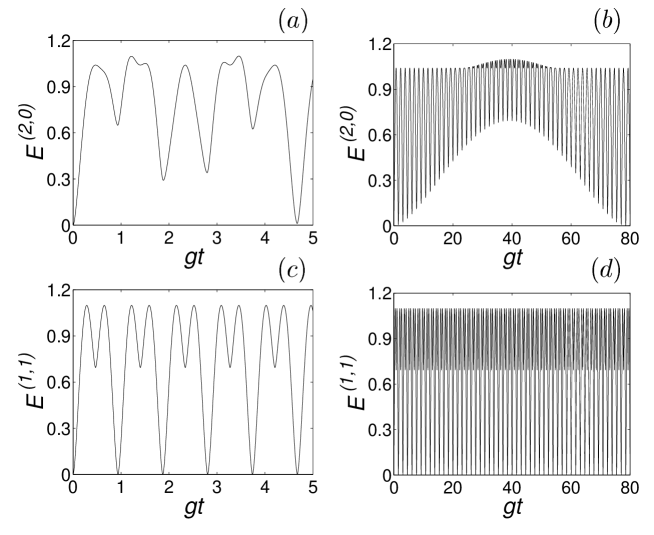
Figure 1: $E^{(2,0)}$ is plotted as a function of $gt$ for (a) $\chi/g=0.34$, (b) $\chi/g=0.01$ when two excitons are initially excited in one of the microcrystallites, and $E^{(1,1)}$ is plotted as a function of $gt$ for (c) $\chi/g=0.34$, (d) $\chi/g=0.01$ when there is one exciton initially in each microcrystallite.

For an arbitrary number of excitons $L$, the wave function of the whole system is described by (14). Then the entropy of the entanglement can be calculated as

$$E^{(L)}(t)\equiv E^{(L,0)}(t)=-\sum_{m^{\prime}=-\frac{L}{2}}^{\frac{L}{2}}|\beta_{m^{\prime}}|^{2}\ln|\beta_{m^{\prime}}|^{2}$$ (20a)

with

$$\beta_{m^{\prime}}=\sum_{m=-\frac{L}{2}}^{\frac{L}{2}}{\cal D}^{\frac{L}{2}}_{\frac{L}{2},m}(\frac{\pi}{2})e^{-\frac{i}{\hbar}E_{\frac{L}{2},m}t}{\cal D}^{\frac{L}{2}}_{m^{\prime},m}(\frac{\pi}{2}),$$ (20b)

where ${\cal D}^{\frac{L}{2}}_{m^{\prime},m}(\frac{\pi}{2})$ is determined by (9).

Equations(20a–20b) are confined to the case of the excitons initially excited in one microcrystallite only. Experimentally, we can also initially excite excitons in both microcrystallites. If $P$ and $Q$ excitons are initially excited in microcrystallites $A$ and $B$ then we have $j=(P+Q)/2$ and $m=(P-Q)/2$, and so the initial state can be expressed as $|\Phi(t=0)\rangle=|P\rangle_{A}|Q\rangle_{B}=|\frac{P+Q}{2},\frac{P-Q}{2}\rangle_{s}$. At time $t$, the wave function of the whole system can be written as

$$|\Phi(t)\rangle = \sum_{l^{\prime}=-(P+Q)/2}^{(P+Q)/2}\exp\Big{(}\frac{t}{i\hbar}E_{\frac{P+Q}{2},l^{\prime}}\Big{)}$$ (21)

$$\times\langle\Psi_{\frac{P+Q}{2},l^{\prime}}|\frac{P+Q}{2},\frac{P-Q}{2}\rangle_{s}|\Psi_{\frac{P+Q}{2},l^{\prime}}\rangle_{s}.$$

We can also obtain the entropy of entanglement for the above initial condition as

$$E^{(P,Q)}(t)=-\sum_{n^{\prime}={-(P+Q)}/2}^{(P+Q)/2}|\beta_{n^{\prime}}^{\prime}|^{2}{\rm ln}|\beta_{n^{\prime}}^{\prime}|^{2}$$ (22a)

with

$$\beta^{\prime}_{n^{\prime}}=\sum_{n=-(P+Q)/2}^{(P+Q)/2}{\cal D}^{\frac{P+Q}{2}}_{\frac{P-Q}{2},n}(\frac{\pi}{2})e^{-\frac{t}{i\hbar}E_{\frac{P+Q}{2},n}}{\cal D}^{\frac{P+Q}{2}}_{n^{\prime},n}(\frac{\pi}{2}).$$ (22b)

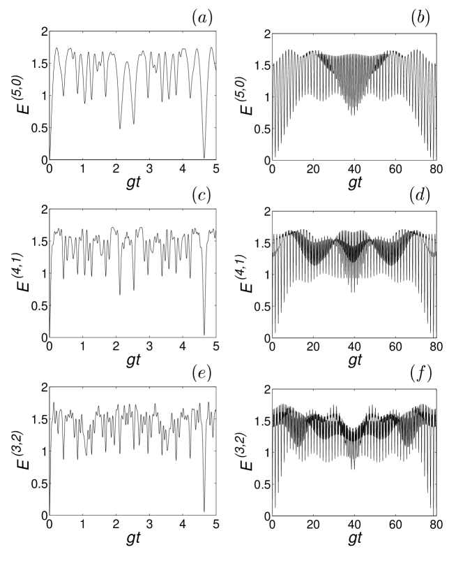
Figure 2: $E^{(5)}\equiv E^{(5,0)}$, $E^{(4,1)}$, and $E^{(3,2)}$ are plotted as a function of $gt$ for $\chi/g=0.34$ (left panel) and $\chi/g=0.01$ (right panel).

Equations (22a–22b) for the entanglement were obtained from the wave function (21) being a complete solution of the model. Thus, the contributions of all elements (also those off-diagonal) of the density matrix are included. In  figure 2, the entropies of the entanglement $E^{(P,Q)}$ are depicted as a function of $gt$ for different exciton numbers $P$ and $Q$ in the first and second microcrystallite, respectively, but for the same total number of five excitons in both microcrystallites. Numerical results show that the evolution behavior of the entropy of the entanglement for $L=5$ is similar to that for $L=2$. However, when we compare the maximum value of the entropy of entanglement with the entropy of the maximally entangled state, we see that a time $t$ at which the generated entangled state is very close to a maximally entangled state cannot be found for any $\chi/g$. The survival time of the maximum entanglement is different for different initial conditions and $\chi/g$. The smaller difference of initial populations corresponds to longer time in a larger entanglement area for fixed $\chi/g$ when the total number of excitons in two microcrystallites is five. We also find that the maximum entanglement for fixed $\chi/g$ is the same for different initial conditions for the total number $L$ of excitons in two microcrystallites $L=2,3$ only, i.e. $E_{\max}^{(2,0)}=E_{\max}^{(1,1)}=E_{\max}^{(0,2)}=\ln 3$ and $E_{\max}^{(3,0)}=E_{\max}^{(2,1)}=E_{\max}^{(1,2)}=E_{\max}^{(0,3)}=2\ln 2$. However, if $L>3$ then $E_{\max}^{(L-n,n)}\neq E_{\max}^{(L-m,m)}$ for $n\neq m\leq L/2$. Nevertheless, the differences are relatively small - only at the second digit after the decimal point, as we have checked numerically up to ten excitons. Concluding, we find that the maximum values of the entropy of entanglement depends both on the initial conditions and on $\chi/g$ when $L>3$.

We can use equations (20a–20b) as an example to further discuss the entanglement of the excitons between the two subsystems $A$ and $B$ of the system for any initially given exciton number. Here the entropy of the entanglement of two subsystems is discussed up to ten excitons. An exact time $t$, which corresponds to a maximally entangled state, can be obtained when the system has one exciton. Numerically up to a evolution time of $gt\leq 600$, when the total number of excitons in our system is two or three, we find that the difference between the maximal entropy of entanglement and the entropy of the maximally entangled state is of the order $10^{-5}$ for $\chi/g\neq 0$. So, the maximally entangled states can be approximately obtained. The maximum values $E^{(L)}_{\rm max}$ of the entropy of the entanglement for the two subsystems are also numerically calculated by using (20a)–(20b) up to the time $gt\leq 600$. Figure 3 shows a comparison of the maximal values $E^{(L)}_{\rm max}$ of the entropy of the entanglement with the values of the entropy of the entanglement for maximally entangled states up to ten excitons for $\chi/g=0,\ 0.01,\ 0.34,\ 0.8$. Figure 3 shows that the entropies of the entanglement for $\chi/g=0$ are smaller than those for $\chi/g=0.01,\ 0.34,\ 0.8$ for all exciton numbers, which means our system can achieve a larger entanglement than that of the linear coupling model. At this point, this coupled microcrystallites system can be considered as a better source of entanglement with a fixed exciton number than that of the linear coupling model with the same particle number. For a fixed exciton number, we find that the difference in the maximum values of the entropies of the entanglement between any two different parameter ratios among $\chi/g=0.01,\ 0.34,\ 0.8$ is very small. Every square in the solid curve of figure 3 actually denotes the maximum values of the entropies of the entanglement for three different values of $\chi/g$. By comparing plots for a small ($\chi/g=0.01$) and a higher ($0.34$) values of the nonlinearity in figures 1, 2, and 3, it is clearly seen that the global maxima of entanglement are practically independent of the ratio of $\chi/g$ (except $\chi/g$), but dependent of the initial conditions. However, higher nonlinearity corresponding to a larger $\chi/g$ enables generation of globally higher entanglement for shorter evolution times.

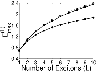
Figure 3: The maximal values $E^{(L)}_{max}$ of the time-dependent von Neumann entropy $E^{(L)}(t)$ are plotted as a function of exciton number $L\leq 10$ for $\chi/g=0$ (dots in solid curve), $\chi/g=0.01$, $0.34$, and $0.8$ (squares in solid curve). The values of the von Neumann entropy of the maximally entangled states are marked by circles in the dotted curve for different exciton numbers $L$.

4 Oscillations of exciton imbalance

In the previous section, we show that the excitonic state of two microcrystallites system has different degree of entanglement with the evolution. The population of the excitons in the microcrystallites $A$ and $B$ is not at equilibrium. The nano-technology opens up a new direction of research for direct measurements of exciton dynamics. Probing one exciton at a time has been demonstrated by using the nonlinear nano-optics [34]. It is possible for experimentalists to observe the population of the excitons in the microcrystallites. Considering that experimentally, it is easier to initially excite excitons in one microcrystallite, in this section our discussions are the case when there are $L$ excitons excited initially in one of the microcrystallites. We will show that the excitonic population imbalance between two coupled microcrystallites exhibits a collapse and revival phenomenon. The time-dependent population difference of excitons between two microcrystallites can be written as

$$\Delta N^{(L)}(t)=N^{(L)}_{1}(t)-N^{(L)}_{2}(t),$$ (23)

where the average exciton number of each microcrystallite $N^{(L)}_{l}(t)=\langle a^{\dagger}_{l}a_{l}\rangle$. The evolution of the population difference of the excitons is similar for different initial conditions. We can discuss the population imbalance of the two microcrystallites using equation (10), but here we only consider the initial condition at which there are $L$ excitons in microcrystallite $A$ and no exciton in microcrystallite $B$. From (14), we can calculate the number of excitons in each microcrystallite as

$$N^{(L)}_{l}(t)=\frac{L}{2}-(-1)^{l}\sum_{m^{\prime}=-\frac{L}{2}}^{\frac{L}{2}}m^{\prime}\left|\beta_{m^{\prime}}\right|^{2},$$ (24)

where $l=1$ represents the microcrystallite $A$ and $l=2$ denotes microcrystallite $B$; time-dependent functions $\beta_{m^{\prime}}$ are given by equation (20b). Then we can obtain the population difference of the excitons between the two microcrystallites as

$$\Delta N^{(L)}(t)=2\sum_{m^{\prime}=-\frac{L}{2}}^{\frac{L}{2}}m^{\prime}\left|\beta_{m^{\prime}}\right|^{2}.$$ (25)

When only one exciton is initially excited in the microcrystallite $A$, the exciton population difference is

$$\Delta N^{(1)}(t)=\cos(2gt),$$ (26)

which is a simple sinusoidal oscillation. The population difference of the exciton is zero at times $gt=(2k+1)\frac{\pi}{4}$, and $\Delta N^{(1)}$ reaches a maximum at times $gt=k\frac{\pi}{2}$, where $k$ is an integer. Comparing this result to equation (16), we know that the two subsystems reach the maximal entanglement when the exciton population difference of the two microcrystallites is zero, but when the entropy of the entanglement of the system is minimum, the population imbalance is maximum.

When there are two excitons initially excited in microcrystallite $A$, we obtain

$$\Delta N^{(2)}(t)=2\cos(4\chi t)\cos[2gt+4\chi t].$$ (27)

Equation (27) indicates that the population difference periodically oscillates with time. We numerically give the evolution of the population difference as a function of $gt$ in figure 4.

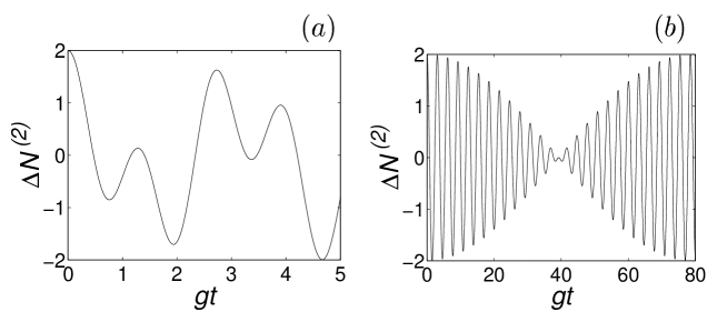
Figure 4: The evolution of the population difference $\Delta N^{(2)}$ between two microcrystallites is shown as a function of $gt$ for (a) $\chi/g=0.34$ and (b) $\chi/g=0.01$.

Figure 4 shows that the exciton population difference of the two microcrystallites exhibits the beat effect. If the second interaction between the excitons becomes weak, the period of the envelope becomes longer than that of the stronger second interaction between excitons.

The general formula for the exciton population difference of two microcrystallites can be given as

$$\Delta N^{(L)}(t)=L\cos^{L-1}(4\chi t)\cos[2gt+4(L-1)\chi t].$$ (28)

With increasing exciton number, the numerical results show that exciton population difference evolution in time resembles a collapse and revival phenomenon. As an example, the evolution of the exciton population difference in a system of the coupled microcrystallites with a total number of $L=5$ excitons is plotted in figure 5 as a function of $gt$. The smaller is the ratio between the second coupling constant and the first coupling constant, the clearer is this phenomenon.

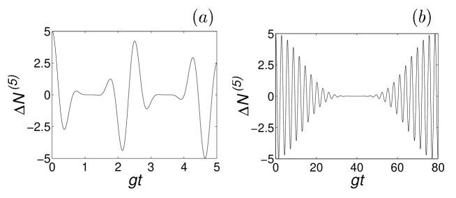
Figure 5: The evolution of the population difference $\Delta N^{(5)}$ between two microcrystallites is shown as a function of $gt$ for (a) $\chi/g=0.34$, and (b) $\chi/g=0.01$.

Figure 6 shows a relationship between the entropy of the entanglement in our system and the exciton-population difference. To estimate the uppermost envelope functions of the curves in figure 6, we apply the Jaynes principle of maximum entropy [35]. In the Jaynes formalism, the entropy can exclusively be expressed in terms of the mean values. The method corresponds to averaging over the generalized grand canonical ensemble of states satisfying given constraints. Thus, the Jaynes formalism of calculating the maximum entropy strongly resembles the standard problems of entropy maximization in statistical mechanics and thermodynamics. It is worth noting that, although the maximum entropy principle “has nothing to do with the laws of physics” [35], it is a useful and widely applied tool in physics, e.g., in the quantum state reconstruction from data obtained in a measurement of a physical process [36]. By applying the Jaynes principle we find the maximum entropy to be expressed as a function of the population difference as

$$E_{J}^{(L)}(\Delta N^{(L)})=-\sum_{n=0}^{L}p_{n}\ln p_{n}=\frac{1}{2}(L+\Delta N^{(L)})\lambda^{(L)}+\ln Z^{(L)},$$ (29)

where $p_{n}=\exp(-n\lambda^{(L)})/Z^{(L)}\equiv x^{n}/Z^{(L)}$ are given in terms of Lagrange multiplier $\lambda^{(L)}$ or $x=\exp(-\lambda^{(L)})$ and the generalized partition function

$$Z^{(L)}=\frac{x^{L+1}-1}{x-1}.$$ (30)

The Lagrange multiplier $\lambda^{(L)}$ can be calculated from

$$\Delta N^{(L)}=f(x)=L+\frac{2}{1-x}-2\frac{1+L}{1-x^{L+1}}.$$ (31)

To obtain an explicit formula for $E_{J}^{(L)}$ one has to find the relation inverse to $\Delta N^{(L)}=f(x)$. By closer inspection of (31), we conclude that the analytical solutions of $x=f^{-1}(\Delta N^{(L)})$ exist only for $L$=2, 3, and 4. For example, the desired solution of $x=f^{-1}(\Delta N^{(2)})$ for $N=2$ is given by

$$x\equiv\exp(-\lambda^{(2)})=\frac{\Delta N^{(2)}+\sqrt{16-3(\Delta N^{(2)})^{2}}}{2(2-\Delta N^{(2)})}.$$ (32)

For brevity, we do not present our analytical, but rather complicated, solutions for $L=3$ and $4$. The solutions for $L\geq 5$ are to be found numerically. The curves marked by circles in figure 6 correspond to our analytical ($L=2,3,4$) and numerical ($L=5$) estimations of the maximum entropy of entanglement as a function of $\Delta N^{(L)}$. It is seen, in agreement with our analysis of figure 3, that with the increasing number $L$ of excitons, the time-maximized entanglement $E^{(L)}_{\max}(t)$, which can be generated in our system, increases in comparison to the lower-exciton systems $E^{(L)}_{\max}(t)>E^{(L-1)}_{\max}(t)$ for the same population difference $\Delta N\equiv\Delta N^{(L)}=\Delta N^{(L-1)}\neq\pm$ $L$ (with any $L$) for a given $\kappa/g$. The states described by $E_{J}^{(L)}(\Delta N^{(L)})$ for $\Delta N=0$ correspond to the maximally entangled states. The numerical results depicted in figure 6 show that the maximum entropy of the entanglement always corresponds to the points of the exciton-population balance. However, the condition of the exciton-population balance does not always imply the maximum entropy of the entanglement. For any population-imbalance points, the entropy of the entanglement is smaller, and when the population difference reaches its maximum, the entropy of the entanglement vanishes.

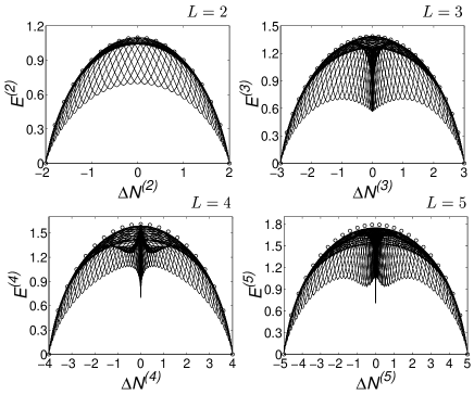
Figure 6: The entropy of entanglement is plotted as a function of the population difference of microcrystallites for $\chi/g=0.34$ when the total number $L$ of excitons is 2, 3, 4, or 5. The uppermost circles represent values estimated by the Jaynes principle.

5 Conclusions

We have discussed the entanglement of the excitonic states in the system of the coupled microcrystallites with a fixed total exciton number by the entropy of the entanglement. When the total number of excitons is one, the maximally entangled state can exactly be obtained. The maximally entangled states can approximately be generated for two or three excitons. However, when the exciton number is more than three, we cannot obtain the maximally entangled state, but it is observed that the nonlinear interaction between excitons increases the maximum values of the entropy of the entanglement to higher values than those of the other models based on the linear coupling. So this exciton system can be used as a good source of entanglement. We also find that the entanglement between the two microcrystallites depends on the initial conditions, the different initial conditions will result in different entanglements.

The oscillations of exciton population between two microcrystallites have also been investigated analytically and numerically. If the system is prepared with one exciton, the population imbalance between two microcrystallites reaches the maximum when the entanglement of the two microcrystallites is the minimum; and the population reaches the balance when the entropy of the entanglement of the system is maximum. But when the exciton number is more than two, the numerical results showed that we could find the maximum entropy of the entanglement at the points of the exciton population balance. At some larger population imbalance points, the entropy of the entanglement was found to be smaller. The reason is that when the population imbalance becomes the largest, all excitons are concentrated on one microcrystallite, then the entanglement between two microcrystallites decreases. But in the collapse area, the average population of each microcrystallite is equal, so it is possible to find the maximal entropy of the entanglement. We hope these phenomena can be observed by experimentalists with the development of the nano-technology.

The main conclusion of our paper is that nonlinear interactions, resulting from high exciton density between microcrystallites, can increase exciton entanglement in comparison to a model of linearly-coupled microcrystallites with lower exciton density. We believe that this result could be important for semiconductor-based quantum information processing. Our conclusion is not only valid for the studied system, but can also be generalized to other Kerr nonlinear vs linear interaction models.

References

References

- [1] Bouwmeester D, Pan J-W, Daniel M, Weinfurter H and Zeilinger A 1997 Nature (London) 390 575
- [2] Furusawa A, Sørensen J I, Braunstein S L, Fuchs C A, Kimble H J and Polzik E S 1998 Science 282 706
- [3] Duan L M, Giedke G, Cirac J I and Zoller P 2000 Phys. Rev. Lett. 84 4002
- [4] [] Duan L M, Giedke G, Cirac J I and Zoller P 2000 Phys. Rev. A 62 032304
- [5] Cochrane P T, Milburn G J and Munro W J 2000 Phys. Rev. A 62 062307
- [6] Barenco A, Deutsh D, Ekert A and Jozsa R 1995 Phys. Rev. Lett. 74 4083
- [7] [] Loss D and DiVincenzo P 1998 Phys. Rev. A 57 120
- [8] [] Imamoǧlu A, Awschalom D D, Burkard G, DiVincenzo D P, Loss D, Sherwin M and Small A 1999 Phys. Rev. Lett. 83 4204
- [9] Oh J H, Ahn D and Hwang S W 2000 Phys. Rev. A 62 052306
- [10] Chen G, Bonadeo N H, Steel D G, Gammon D, Katzer D S, Park D and Sham L J 2000 Science 289 1906
- [11] Bayer M, Hawrylak P, Hinzer K, Fafard S, Korkusinski M, Wasilewski Z R, Stern O and Forchel A 2001 Science 291 451
- [12] Quiroga L and Johnson N F 1999 Phys. Rev. Lett. 83 2270
- [13] [] Reina J H, Quiroga L and Johnson N F 2000 Phys. Rev. A 62 012305
- [14] Yi X X, Jin G R, Zhou D L 2001 Phys. Rev. A 63 062307
- [15] Miranowicz A, Özdemir Ş K, Liu Yu-xi, Koashi M, Imoto N and Hirayama Y 2002 Phys. Rev. A 65 062321
- [16] Wang X, Feng M and Sanders B C 2003 Phys. Rev. A 67 022302
- [17] Livermore C, Crouch C H, Westervelt R M, Campman K L and Gossard A C 1996 Science 274 1332
- [18] Fujisawa T, Oosterkamp T H, van der Wiel W G, Broer B W, Aguado R, Tarucha S, Kouwenhoven L P 1998 Science 282 932
- [19] [] Oosterkamp T H, Fujisawa T, van der Wiel W G, Ishibashi K, Hijman R V, Tarucha S and Kouwenhoven L P 1998 Nature 395 873
- [20] Hanamura E 1988 Phys Rev B 38 1228
- [21] Belleguie L and Bányai L 1991 Phys. Rev. B 44 8785
- [22] [] Bányai L and Koch S W 1993 Semiconductor Quantum Dots (Singapore: World Scientific)
- [23] Engelmann A, Yudson V I and Reineker P 1998 Phys. Rev. B 57 1784
- [24] Liu Yu-xi, Özdemir S K, Koashi M and Imoto N 2002 Phys. Rev. A 65 042326
- [25] [] Liu Yu-xi, Miranowicz A, Koashi M and Imoto N 2002 Phys. Rev. A 66 062309
- [26] [] Liu Yu-xi, Miranowicz A, Özdemir S K, Koashi M and Imoto N 2003 Phys. Rev. A 67 034303
- [27] Chernyak V and Mukamel S 1996 J. Opt. Soc. Am. B 13 1302
- [28] Schwinger J 1965, US Atomic Energy Commission Report No. NYO-3071 (US GPO, Washington, D.C.); reprinted in Biedenharn L C and van Dam H (eds) 1965 Quantum Theory of Angular Momentum (New York: Academic) p 229
- [29] Sakurai J J 1994 Modern Quantum Mechanics (New York: Addison-Wesley)
- [30] Bennett C H, Bernstein H J, Popescu S, and Schumacher B 1996 Phys. Rev. A 53 2046
- [31] Bennett C H, DiVincenzo D P, Smolin J A, and Wootters W K 1996 Phys. Rev. A 54 3824
- [32] Vedral V and Plenio M B 1998 Phys. Rev. A 57 1619
- [33] Phoenix S J D and Knight P L 1991 Phys. Rev. A 44 6023; 1991 Phys. Rev. Lett. 66 2833; 1988 Ann. Phys. 186 381
- [34] Bonadeo N H, Chen Gang, Gammon D, Katzer D S, Park D and Steel D G 1998 Phys. Rev. Lett. 81 2759
- [35] Jaynes E T 1957 Phys. Rev. 106 620; 108 171
- [36] Bužek V, Adam G and Drobný G 1996 Phys. Rev. A 54 804