Triggered qutrits for Quantum Communication protocols

Abstract

A general protocol in Quantum Information and Communication relies in the ability of producing, transmitting and reconstructing, in general, qunits. In this letter we show for the first time the experimental implementation of these three basic steps on a pure state in a three dimensional space, by means of the orbital angular momentum of the photons. The reconstruction of the qutrit is performed with tomographic techniques and a Maximum-Likelihood estimation method. In this way we also demonstrate that we can perform any transformation in the three dimensional space.

One of the main objectives in Quantum Information is exploring the possibilities of applying quantum systems in communication and computation protocols. Usually, these protocols use the information encoded in two dimensional systems, better known as qubits. Nevertheless, some proposals show that higher dimensional systems are better suited for certain purposes Bourennane01a ; Bechmann00a ; Bechmann00b ; Divincenzo00a ; Bartlett00a ; Karimipour01a ; Ambainis01a ; Bruknercomplex03 . On a more fundamental level, higher dimensional Hilbert spaces provide novel counter-intuitive examples of the relationship between the quantum and the classical information, which cannot be found in two-dimensional systems Jozsa00 .

Encoding qunits (systems with $n$ different orthogonal states) with photons has been experimentally demonstrated using interferometric techniques, such as time-bin schemes Riedmatten02QIC and superpositions of spatial modes Zukowski97multiport . Up to now, the only non-interferometric technique of encoding qunits in photons is using their orbital angular momentum or, equivalently, their transversal modes Mair01a ; Molina-Terriza02 . Orbital angular momentum modes usually contain dark spots which regularly exhibit phase singularities.

The orbital angular momentum of light has already been used to entangle and concentrate the entanglement of two photons Mair01a ; Vaziri03a . This entanglement has also been shown to violate a two particle three-dimensional Bell inequality Vaziri02b . There have been proposals of some experimental techniques to engineer entangled qunits in photons Molina-Terriza02 ; Torres03a ; Vaziri02a . In this paper we experimentally demonstrate all the basic steps of a higher dimensional quantum communication protocol.

In a general communication scheme, prior to the sharing of information, the two parties, say Alice and Bob, have to define a procedure which will assure that the signal sent by one party is properly received by the other one. Usually, this scheme works as follows: First, Alice prepares a signal state she wants to send. Bob will measure it and communicate the result to Alice, who will correct the parameters of her sending device following Bob’s indications. This process will repeat itself until the two parties adjust the corresponding devices. After this step is fulfilled, Alice can rely that any subsequent signal which is sent is properly received.

Using pairs of photons entangled in orbital angular momentum, we can prepare any qutrit state, transmit it, and measure it. The preparation is done by projecting one of the two photons onto some desired state. This nonlocally projects the second photon onto a corresponding state. This state may be transmitted to Bob and finally measured by him. The measurement employs tomographic reconstruction. This last step is usually a technically demanding problem, inasmuch as it needs the implementation and control of arbitrary transformations in the quantum system’s Hilbert space.

On theoretical grounds, one convenient basis which describes the transversal modes of a light beam fulfilling the paraxial approximation is the Laguerre-Gaussian (LG) functions basis: $LG_{p,m}(x,y)$. Here $m$ is the order of the phase dislocation characteristic of this set of functions and it accounts directly for the orbital angular momentum of the Laguerre-Gaussian mode in units of $\hbar$Allen92a ; He95a . The other parameter $p$ is a label which is related to the number of radial nodes of the mode and $(x,y)$ refer to any point in a plane perpendicular to the beam propagation direction. The LG functions form a complete and orthonormal basis for any complex function in the transveral plane.

Holographic techniques can be used to transform $LG$ modes Bazhenov90a . Conveniently prepared holograms change the phase structure of the incoming beam, adding or removing the phase dislocations related with the orbital angular momentum. Whereas optical single mode fibers act as a filter for all higher $LG$ modes, i.e. only the $LG_{00}$, or Gaussian, mode can be transmitted, the combination of holograms and single mode fibers project the incoming photon into different states. In this way we can define the basis of the experimentally accessible states as:

$$\langle\vec{x}|0\rangle=LG_{0,0}(x,y),~{}|m\rangle=H_{m}(\vec{0})|0\rangle,$$ (1)

where the vector $|0\rangle$ is the mode of the fiber used to detect the photon, $\vec{x}$ is a shortcut to represent any point in the transversal space, $m$ is a positive or negative integer, and $H_{m}(\vec{0})$ is the operator which describes the action of the $m$-th order hologram when it’s centered, relative to the fiber.

Although the mode $|m\rangle$ posses orbital angular momentum of $m\hbar$, they are not pure $LG$-modes. However, they can be described as coherent superpositions of different $LG$-modes with the same $m$, but different $p$’s. In this sense, the basis we have constructed in (1) is not complete, since it does not expand the $LG$ basis. In the following we refer to all modes belonging to the subspace (1) as “inner” modes and the rest of the modes will be addressed as “outer” modes.

Thus, any displaced hologram and, in general, any linear operator which acts on our Hilbert space can be expressed like $H_{m}(a,b)=\sum_{i=-\infty}^{+\infty}c_{i}(a,b)H_{i}(0)+\gamma(a,b)\Gamma$ where $a,b$ are the displacements of the hologram along the orthogonal directions in the transversal plane, relative to its centered position. The operator $\Gamma$ accounts for the possibility that the displaced hologram is performing transformations between “outer” and “inner” states, i.e. transforming any “inner” state into an “outer” one, or the other way round.

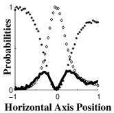
Figure 1: Effect of a hologram on an initially prepared $|0\rangle$ mode. This mode is transformed by means of a horizontally displaced hologram of charge $m=+1$. The resulting state is projected onto the basis states. In this case the modes $|0\rangle$ and $|1\rangle$ are expected to contribute the most to the transformed state. Asterisks: projection onto the $|0\rangle$ mode. Diamonds: projection onto the $|1\rangle$ mode. The solid line represents the projection onto “outer” the modes, i.e. those not belonging to the basis (1). This projection is found by subtracting to the total number of events those corresponding to the projection onto the elements of the basis. The two positions of the hologram where the transfer to “outer” modes is maximum are taken as new elements of the basis.

The value of $\gamma$ can be estimated experimentally. In Fig. 1 we present an example of such a measurement. It is observed how there are two positions where the contribution of the “outer” modes is specially high.

Up to now the most convenient way of transforming an OAM state is to employ holograms. Yet, as discussed above, these holograms might also perform unsought transformations between “inner” and “outer” modes. To avoid this problem we enlarge our Hilbert space with some selected “outer” vectors. We choose eight different positions of the holograms as new operators which, together with a projection into the $|0\rangle$ mode and a Gram-Schmidt orthonormalization, enlarge our natural Hilbert space. In the present work we enlarged the basis with four positions for every differently charged hologram used in the experiment. Each of this four points correspond to the two vertical and the two horizontal positions where the probability of transforming a state of the basis into an“outer” mode is bigger.

The enlargement of the basis (1) allow us to represent more precisely the effect of the hologram on our beam but, as a drawback we need more measurements to estimate the state of the photon, as there are more dimensions in our Hilbert space. This problem, considered together with the imperfections of the holograms and possible systematic drifts due to experimental misalignments during the measurements, makes it a natural option to turn to maximum likelihood (ML) schemes for reconstructing the transformed states.

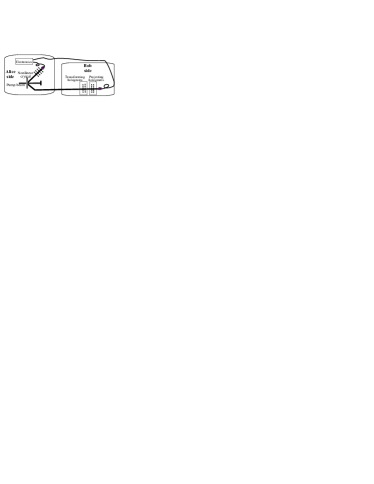
Figure 2: Experimental set-up. A $351$nm wavelength laser pumps a BBO crystal. The two generated $702$nm down-converted photons are send to Alice and Bob’s detectors respectively. Before being detected each photon propagates through a set of holograms. Each photon was coupled into single mode fibers and directed to detectors based on avalanche photo diodes operating in the photon counting regime.

The experimental set-up it is shown in Fig. 2 . A $351$nm wavelength Argon-ion laser pumps a $1.5-$mm-thick BBO ($\beta$-barium-borate) crystal cut for Type I phase matching conditions. The crystal is positioned such as to produce down-converted pairs of equally polarized photons at a wavelength of $702$nm emitted at an angle of $4^{\circ}$ off the pump direction. These photons are directly entangled in the orbital angular momentum degree of freedom. Alice can manipulate one of the downconverted photons, while the other is sent to Bob. Before being detected, Bob’s photon traverses two sets of holograms. Each set consists of one hologram with charge $m=1$ and another with charge $m=-1$. The first set of holograms provides the means of a transformation in the three dimensional space expanded by the states $|-1\rangle,|0\rangle$ and $|1\rangle$. The second set, together with a single mode fiber and a detector, act as a projector onto the three different basis states. All this elements are Bob’s receiving device. Alice’s photon also traverses a set of holograms, which together with the source, and the detector on Alice side, act as Alice’s sending device. Whenever Alice detects one photon, this initiates the transmission of a photon to Bob. By means of the quantum correlations between the entangled photons, Alice can radically control the state of the photon sent to Bob. In order to adjust properly their respective devices, Bob has to perform a tomographic measurement of the state he is receiving and classically communicate to Alice the result.

In our experiment, the tomographic reconstruction of Bob’s received qutrit state was realized in two independent steps trying to avoid any bias from ‘a priori’ information. First, the Vienna team by measuring Alice’s photon projected the photons in Bob’s side and then performed the required measures. The minimum number of measurements to reconstruct the three dimensional state sent to Bob is $9$. This number increases to $121$ for our enlargement to a $11$-dimensional Hilbert space. In the end, to exploit the power of the ML reconstruction and to minimize errors, the number of different projections was around $2400$. The results of these measurements, together with the projecting vectors, were sent to the Olomouc team who, without a previous knowledge of which was the state projected by Alice, reconstructed the density matrix describing the state of the photon in Bob’s side. As will be shown below in all the cases the reconstructed three dimensional state was a coherent superposition of the three “inner” vectors, whose relative weights and phases could be effectively controlled demonstrating that any qutrit state could be sent. The noise and incoherence were within the Poissonian noise level, which is an indication of the reliability of the tomographic measurement.

The transforming set of holograms was analyzed to properly describe the transformation done. From the description of each single hologram, we could express the action of each transformation set in the following way:

$$\begin{split}&\langle\vec{x_{1}}|H_{1}(a_{+1},b_{+1})H_{-1}(a_{-1},b_{-1})|\vec{x_{2}}\rangle=\\ &\exp(-i\arctan(\frac{y_{1}-a_{1}}{x_{1}-b_{1}})+i\arctan(\frac{y_{1}-a_{-1}}{x_{1}-b_{-1}})\\ &-ik_{x}x_{1}-ik_{y}y_{1})\delta(x_{1}-x_{2},y_{1}-y_{2})\end{split}$$

where $k_{x}$ and $k_{y}$ are free parameters which depend on the alignment procedure and on the holographic grating, and $a_{\pm}1,b_{\pm}1$ represent the displacement of the two holograms. Each set of holograms is described completely by eight parameters: the number of maximum coincidences, the width of the beam, $4$ numbers to determine the centered position of each hologram and the two parameters $k_{x}$ and $k_{y}$.

The estimation of these eight parameters was performed by fitting four different experimental curves. The data which conformed the curves were taken by sending to Bob a photon prepared in the $|0\rangle$ state. Bob fixed one of his holograms in one determined position and performed a scan on one of the axes of the other hologram. The resulting state was again projected to the $|0\rangle$ state, i.e. one of this curves can be described by $\langle 0|H_{1}(x,0)H_{-1}(1,1)|0\rangle$ as a function of $x$. Each of the four curves corresponds to the scan of all the axes of the two holograms.

The projection measurements were made by moving the transformation set of two holograms into around $2400$ different positions and counting the number of coincident detections which took place in 2 seconds. For every position, we counted typically a few hundred of coincidences per second. The complete time for each of this measurements was around 6 hours. After this time some slight misalignments where detected, which could be compensated mainly due to the large number of different projections taken and the reconstruction process

The registered data were processed using the maximum-likelihood (ML) reconstruction algorithm. Assuming that the statistics of the detection events at low intensities is Poissonian, the joint probability of observing registered data reads,

$${\cal L}=\prod_{j}(Np_{j})^{n_{j}}e^{-Np_{j}}/n_{j}!,$$ (2)

where $N$ is the mean number of qutrits subject to each measurement of which $n_{j}$ were found in the state $|j\rangle=H_{1}(a^{j}_{+1},b^{j}_{+1})H_{-1}(a^{j}_{-1},b^{j}_{-1})|0\rangle$, and $p_{j}=\mathrm{Tr}\{|j\rangle\langle j|\rho_{\mathrm{Bob}}\}$ are the corresponding probabilities.

In accordance with the Bayes theorem Bayes-class , $\mathcal{L}$ quantifies the likelihood of Bob’s state $\rho_{\mathrm{Bob}}$ in view of the measured data. The state having highest likelihood is picked up as the result of the reconstruction. ML estimation is known to be asymptotically efficient fisher ; Helstrom and all existing physical constraints such as positivity of $\rho$ can easily be incorporated into the reconstruction process.

From the technical point of view the maximum of functional (2) is found by iterating the extremal equation, Rehacek01 $R\rho R=G\rho G$ starting from the maximally mixed state. Hermitian operators $R=\sum_{j}(n_{j}/p_{j})|j\rangle\langle j|$ and $G=(\sum_{j}n_{j})/(\sum_{j}p_{j})\sum_{j}|j\rangle\langle j|$ are functions of the measurements and detected data.

Let us mention that though the reconstruction is done on the full $3+8$ dimensional Hilbert space spanned by the “inner” and “outer” states, we are interested only in the “inner” subspace. Therefore all the reconstructed states are projected to this subspace to simplify the discussion.

As we have already explained, different projections done by Alice translate through the entanglement into different state preparations on Bob’s side. Three such remote preparations are shown in Fig. 3.

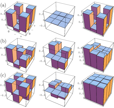
Figure 3: Results of quantum state tomography applied to three different remotely prepared states of Bob’s qutrits:(a) $0.68|0\rangle+0.71|1\rangle-0.14|\text{--1}\rangle$; (b) $0.65|0\rangle+0.53\exp(-i0.26\pi)|1\rangle+0.55\exp(-i0.6\pi)|\text{--1}\rangle$; (c) $0.58|0\rangle+0.58\exp(-i.05\pi)|1\rangle+0.58\exp(-i.89\pi)|\text{--1}\rangle$. Left and middle panels show real and imaginary parts of the reconstructed density matrices; right panels visualize the absolute values of those elements for better comparison of how large are the contributions of the three basic states. From the results it is shown that Alice can control both the relative amplitudes and phases of the sent states.

All of them were found to be very nearly pure states, their largest eigenvalues and corresponding eigenvectors being (a) $\lambda_{max}=0.99$, $|e_{max}\rangle=0.68|0\rangle+0.71|1\rangle-0.14|-1\rangle$; (b) $\lambda_{max}=0.99$, $|e_{max}\rangle=0.65|0\rangle+0.53\exp(-i0.26\pi)|1\rangle+0.55\exp(-i0.6\pi)|-1\rangle$; (c) $\lambda_{max}=0.99$, $|e_{max}\rangle=0.58|0\rangle+0.58\exp(-i0.05\pi)|1\rangle+0.58\exp(-i0.89\pi)|-1\rangle$. In case (a) Alice tried to prepare an equal-weight superposition of $|0\rangle$ and $|-1\rangle$ basis states. Utilizing the conservation of the orbital momentum in downconversion, this was easily done by projecting her qutrit along the ray $|0\rangle+|1\rangle$: Her hologram with the positive charge was taken out of the beam path and the center of the other one was displaced with respect to the beam by a determined translation vector. Cases (b) and (c) both represent an equal-weight superposition of the three states, but with different relative phases, showing that besides the relative intensities, we could also control the relative phases. Other qutrits reconstructed (not shown in Fig. 3), showed an effective suppression of the $|0\rangle$ mode, through destructive interference from the two holograms. The result was $\lambda_{max}=0.97$, $|e_{max}\rangle=0.26|0\rangle+0.68\exp(i0.11\pi)|1\rangle+0.68\exp(-i0.21\pi)|-1\rangle$.

As can be deduced from the maximum eigenvalue of all the data, the purity of the reconstructed states was over $97\%$. On the other hand, by direct comparison of the measured data and the data estimated by the reconstructed matrix, the error was comparable to the statistical Poissonian noise, which demonstrates the reliability of the tomography.

In conclusion, here we have demonstrated the feasibility of a point to point communication protocol in a three-dimensional alphabet. Using the orbital angular momentum of photons, we have implemented three basic tasks inherent in any communication or computing protocol: preparation, transmission and reconstruction of a qutrit. In particular, the reconstruction was exercised with a tomographic estimation of the density matrix, which also demonstrates that we could perform any rotation of the states.

This work was supported by the Austrian Science Foundation (FWF), project number SFB 015 P06, by project LN00A015 of the Czech Ministry of Education, and by the European Commission, contract no. IST-2001-38864, RAMBOQ. G.M.-T. is a Marie Curie Fellowship.

References

- (1) M. Bourennane, A. Karlsson, and G. Björk, Phys. Rev. A 64, 012306 (2001).
- (2) H. Bechmann-Pasquinucci and A. Peres, Phys. Rev. Lett. 85, 3313 (2000).
- (3) H. Bechmann-Pasquinucci and W. Tittel, Phys. Rev. A 61, 62308 (2000).
- (4) D. P. DiVincenzo, T. Mor, P. W. Shor, J. A. Smolin, and B. M. Terhal, Comm. Math. Phys. 238, 379 (2003).
- (5) S. D. Bartlett, H. de Guise, and B. C. Sanders, Proceedings of IQC’01, 344 (2001). quant-ph/0011080.
- (6) V. Karimipour, S. Bagherinezhad, and A. Bahraminasab, Phys. Rev. A 65, 042320 (2002).
- (7) Andris Ambainis, Proceedings of STOC, pages 134–142 (2001).
- (8) C. Brukner, M. Zukowski and A. Zeilinger, Phys. Rev. Lett. 89, 197901 (2002).
- (9) R. Jozsa, and J. Schlienz, Phys. Rev. A 62, 012301 (2000).
- (10) H. de Riedmatten, I. Marcikic, H. Zbinden and N. Gisin, Quantum Information and Computation 2, 425 (2002).
- (11) M. Zukowski, A. Zeilinger, M. A. Horne, Phys. Rev. A 55, 2564 (1997).
- (12) A. Mair, A. Vaziri, G. Weihs, and A. Zeilinger, Nature 412, 313 (2001).
- (13) G. Molina-Terriza, J. P. Torres and L. Torner, Phys. Rev. Lett. 88, 013601 (2002).
- (14) A. Vaziri, J. W. Pan, T. Jennewein, G. Weihs and A. Zeilinger. quant-ph/0303003.
- (15) A. Vaziri, G. Weihs and A. Zeilinger, Phys. Rev. Lett., 89, 240401 (2002).
- (16) A. Vaziri, G. Weihs, and A. Zeilinger, J. Opt. B: Quantum Semiclass. 4, S47–S50 (2002).
- (17) J. P. Torres, Y. Deyanova, L. Torner and G. Molina-Terriza, Phys. Rev. A 67, 052313 (2003). J. P. Torres, A. Alexandrescu and L. Torner, quant-ph/0306105.
- (18) L. Allen, M. W. Beijersbergen, R. J. C. Spreeuw, and J. P. Woerdman, Phys. Rev. A 45, 8185 (1992).
- (19) H. He, M.E. Friese, N.R. Heckenberg, and H. Rubinsztein-Dunlop, Phys. Rev. Lett. 75, 826 (1995).
- (20) V. Yu Bazhenov, M. V. Vasnetsov, and M. S. Soskin, JETP Lett. 52, 429 (1990). N. R. Heckenberg, R. McDu., C. P. Smith, and A. G. White., Opt. Lett. 17, 221 (1992).
- (21) J. M. Bernardo and A. F. M. Smith, “Bayesian Theory” (Wiley, Chichester, 1994).
- (22) R.A. Fisher, Proc. Camb. Phi. Soc. 22, 700 (1925).
- (23) C. W. Helstrom, Quantum Detection and Estimation Theory, (Academic Press, New York 1976).
- (24) J. Řeháček, Z. Hradil, and M. Ježek, Phys. Rev. A 63, 040303(R) (2001).