Signatures of wave packet revival phenomena in the expectation values of observables

Abstract

Wave packet revivals and fractional revivals are striking quantum interference phenomena that can occur under suitable conditions in a system with a nonlinear spectrum. In the framework of a specific model (the propagation of an initially coherent wave packet in a Kerr-like medium), it is shown that distinctive signatures of these revivals and fractional revivals are displayed by the time evolution of the expectation values of physical observables and their powers, i.e., by experimentally measurable quantities. Moreover, different fractional revivals can be selectively identified by examining appropriate higher moments.

I Introduction

It is well known that the dynamics of a quantum wave packet whose evolution is governed by a nonlinear Hamiltonian can display a variety of non-classical effectswall ,drum , arising from the interference between the stationary states comprising the wave packet. These effects manifest themselves through several interesting observable phenomena such as revivals, fractional revivals and super-revivals of the wave packet at specific instants of timepark -bann . Such revivals have been identified in several physical systems. The phenomenon has been observed experimentally and investigated theoretically in a wide class of suitably prepared states subject to specific nonlinear potentials, including Rydberg wave packetspark -meac and molecular vibrational statesvrak ,dool . For a recent comprehensive review of revival phenomena, see robi .

Detailed calculations have been made on revival times within the framework of the Jaynes-Cummings model of a two-level atom interacting with a single mode of electromagnetic radiationeber ,aver2 . Full and fractional revivals of angular momentum coherent statesrozm , $SU(1,1)$ coherent statesbann , states evolving in specific one-dimensional potentials like the infinite square wellaron , and general multi-level quantum systemsleic have also been studied.

The non-classical effects that arise in the dynamics of specific wave packets evolving in a Kerr mediumyurk , collapse and revival phenomena displayed by a single-mode field propagating in a nonlinear mediumagar , and the temporal behavior of a macroscopic superposition of coherent states governed by a nonlinear Hamiltoniantara have been reported upon. An interesting analogy between revivals of wave packets and Poincaré recurrences in classical maps has also been pointed out, and the interplay between revivals, recurrences and geometric phases has been elucidated sesh1 , sesh2 .

Much of the attention given to the revival phenomenon has been with a view to understanding the precise nature of the transition from quantum to classical dynamics, and the deviations from classical predictions that are displayed during the long-time evolution of quantum states. Wave packets prepared so as to satisfy the minimum uncertainty condition at the initial instant of time are clearly appropriate candidates for this purpose. A Rydberg state (an electron excited to a high energy level in the bound-state spectrum by the application of a suitable laser pulse), for instance, is well described by a wave packet which is sharply peaked about a large quantum number $n_{0}$, and the spectrum is approximately linear in this energy region. Although such a wave packet generally spreads with time, it can display, under special circumstances, complete or full revivals as well as fractional revivals at specific instants of time during its evolution.

What has emerged from both experimental and theoretical investigations of this phenomenon is the following: the broad features of wave packet dynamics are quite generic, regardless of the details of the physical system concerned, the initial wave packet considered, and the specific nonlinear Hamiltonian governing its time evolution. Given an initial state $\left|{\psi(0)}\right\rangle$, if the overlap function $C(t)=\left|\langle\psi(0)|\psi(t)\rangle\right|^{2}$ returns to its initial value of unity at specific instants of time, we have a revival. Revival phenomena are essentially controlled by the parameters occurring in the first- and second-order terms in the Taylor expansion of the energy spectrum $E_{n}$ about the energy $E_{n_{0}}$ corresponding to the peak of the wave packet, namely,

$$E_{n}-E_{n_{0}}=\sum_{m=1}^{\infty}\frac{1}{m!}\left[\frac{d^{m}E_{n}}{dn^{m}}\right]_{n=n_{0}}(n-n_{0})^{m}.$$ (1)

The quadratic term in Eq. (1) can also lead to fractional revivals that occur at specific instants between two successive revivals of the wave packet. At these times the initial wave packet evolves to a state that can be described as a collection of spatially distributed sub-packets, each of which closely resembles the initial wave packet. Since each of the basis states comprising the wave packet acquires a different phase during its temporal evolution, in general, fractional revivals can occur only if the numerical values of the parameters that appear in the Hamiltonian satisfy certain conditions, namely, if certain ratios of these parameters are sufficiently close to rational numbers. Anharmonic corrections due to the cubic and higher order contributions in Eq. (1), leading to so-called super-revivals, have also been investigated, in particular in the context of Rydberg atoms bluh2 ,leic ,knos ,brau1 . For wave packets which are peaked sufficiently sharply about $E_{n_{0}}$, these higher order effects that occur on comparatively longer time scales are negligible.

While it is evident that revivals and fractional revivals are genuinely quantum mechanical in origin, it is of interest to examine the signatures of these phenomena in experimentally measurable quantities, i.e., upon the expectation values of appropriate physical observablesbrau2 . More specifically, we are concerned with the possibility of finding distinctive signatures of different fractional revivals occurring between successive revivals that would enable one to distinguish between them unambiguously. In this paper, we use the example of a specific nonlinear Hamiltonian that is both physically relevant and for which analytic calculations can be performed, to show that this is indeed feasible. This implies that revival phenomena can be investigated directly, in terms of these experimentally accessible expectation values.

The plan of the paper is as follows: In the next section we briefly outline the salient aspects of revivals and fractional revivals relevant to our purposes, including the relationship between the time of occurrence of a specific fractional revival and the number of spatially distributed sub-packets representing the state at that instant of time. In Section III we obtain expressions for the mean and higher moments of the position and momentum operators and track their behavior as the wave packet evolves in time. This helps us identify the distinguishing features displayed by these quantities at the instants when fractional revivals occur. We conclude with a discussion of our results in Section IV.

II Revivals and fractional revivals

Consider a nonlinear time-independent Hamiltonian $H$ with a non-degenerate spectrum $\{E_{n}\}$ and eigenstates $\{\left|{\phi_{n}}\right\rangle\}$. The initial state $\left|{\psi(0)}\right\rangle$ in which the system is prepared is a superposition of these eigenstates, sharply peaked about some $n_{0}$. For ease of notation we shift $n$ by $n_{0}$ in Eq. (1), and retain terms up to second order in $r=n-n_{0}$, since only these terms contribute to revivals and fractional revivals. The unitary time evolution operator $U(t)=\exp\,(-iHt/\hbar)$ can be written in the natural basis in standard notationrobi as

$$U(t)=\sum_{r}\exp\,\left\{-2\pi it\left(\frac{r}{T_{\rm cl}}+\frac{r^{2}}{T_{\rm rev}}\right)\right\}\,\left|{\phi_{r}}\right\rangle\left\langle{\phi_{r}}\right|,$$ (2)

apart from an overall phase factor. Here $T_{\rm cl}=h/|E^{\prime}(n_{0})|$ and $T_{\rm rev}=2h/|E^{\prime\prime}(n_{0})|$. The quadratic term in the exponent is responsible for the spreading and distortion of the initial wave packet. However, if there exist specific instants of time such that, for every $r$ in the summation, the exponent is equal to an integer multiple of $2\pi i$, then $U(t)$ reduces to the identity operator apart from an overall phase factor, and a revival occurs. Further, as mentioned in Sec. I, fractional revivals can occur at certain instants of time in between successive revivals. In general, exact revivals require special values of the ratio $T_{\rm cl}/T_{\rm rev}$, but generically $C(t)$ can take on values arbitrarily close to unity at certain instants of timesesh1 . In some sense, such revivals may be regarded as analogs of Poincaré recurrences of a classical dynamical system in a coarse-grained phase space.

For definiteness, we shall consider in the rest of this paper the example of wave packet evolution in a Kerr-like medium. The relevant physics of this situation is captured by the model Hamiltonianagar ,kita

$$H=\hbar\chi\,a^{\dagger 2}\,a^{2}=\hbar\chi\,N(N-1)$$ (3)

in the usual notation, with $N=a^{\dagger}\,a,\,\chi=\,$ positive constant. Essentially the same spectrum modelsgrei the interaction energy of the atoms in a Bose-Einstein condensate. The initial state $\left|{\psi(0)}\right\rangle$ is taken to be the oscillator coherent state $\left|{\alpha}\right\rangle$ (where $\alpha\in\mathbb{C}$), as it is a minimum position-momentum uncertainty state, and hence is “classical” in this sense. The corresponding position-space and momentum-space wave functions are Gaussian wave packets. Owing to the nonlinear nature of $H$, these wave packets not only spread out as $t$ increases, but also change shape, and the state loses its coherence property. We have $U(t)=\sum_{0}^{\infty}\exp\,[-i\chi n(n-1)t]\left|{n}\right\rangle\left\langle{n}\right|$, where $\left|{n}\right\rangle$ denotes the usual number operator eigenstate. Since $n(n-1)$ is always an even integer, it is evident that $T_{\rm cl}=T_{\rm rev}=\pi/\chi$ in this case.

In between $t=0$ and $t=T_{\rm rev}$, fractional revivals occur at times $t=\pi l/m\chi$, where $m=2,3,4,\ldots$, and $l=1,2,\ldots,(m-1)$ for a given value of $m$. This can be traced to the interesting periodicity property exhibited by $U$ at these instants of time, consequent to which it can be Fourier expanded in the basis set $\{\exp\,(-2\pi il/m),\,0\leq l\leq(m-1)\}$ for each $m$. Writing

$$\left|{\psi(t)}\right\rangle=e^{-\left|{\alpha}\right|^{2}/2}\sum_{n=0}^{\infty}\frac{e^{-i\chi n(n-1)t}\,\alpha^{n}}{\sqrt{n!}}\left|{n}\right\rangle$$ (4)

we see that, at these instants of time, the exponential in the summand can be absorbed in the complex number $\alpha$. Thus $\left|{\psi(\pi/m\chi)}\right\rangle\equiv\left|{\psi_{m}}\right\rangle$ becomes a finite superposition of “rotated” coherent states with definite amplitudes, according to

$$\left|{\psi_{m}}\right\rangle=\left\{\begin{array}[]{ll}\sum_{l=0}^{m-1}f_{l}\left|{\alpha\,e^{-2\pi il/m}}\right\rangle,&m\,{\rm odd}\\[10.0pt] \sum_{l=0}^{m-1}g_{l}\left|{\alpha\,e^{i\pi/m}\,e^{-2\pi il/m}}\right\rangle,&m\,{\rm even,}\end{array}\right.$$ (5)

where $f_{l}$ and $g_{l}$ are the Fourier coefficients. For instance, the state at time $\pi/(2\chi)$ (corresponding to $m=2$) is a superposition of the two coherent states $\left|{i\alpha}\right\rangle$ and $\left|{-i\alpha}\right\rangle$. In general, $\left|{\psi_{m}}\right\rangle$ is a superposition of $m$ coherent states. The corresponding wave packet in position space is a superposition of $m$ spatially distributed Gaussian wave packets, and a fractional revival is said to have occurred. The periodicity property of $U$ further implies that the wave function at times $t=\pi l/m\chi,\,1\leq l\leq m-1,$ is also a superposition of $m$ wave packetsaver1 . It is therefore clear that experimental observations of fractional revivals that depend on probing the wave packet itself are quite involved and somewhat indirect, and careful interpretation of the results is required before firm conclusions can be drawn. It is this aspect that leads us to suggest that an examination of the moments of observables may provide a less intricate and more definitive means of identifying and sorting out revival phenomena.

III Moments of observables

We now show how fractional revivals are mirrored, in distinctive ways, in the expectation values of the physical observables pertaining to the system. As the system enjoys revivals with a period $T_{\rm rev}$, all such expectation values are periodic functions of $t$ with this fundamental period.

The relevant observables are the position $x=(a+a^{\dagger})/\sqrt{2}$ and $p=(a-a^{\dagger})/i\sqrt{2}$. Clearly, their expectation values alone do not suffice to reproduce the full information contained in the wave function itself. In principle, an infinite set of moments, namely, the expectation values of all powers of $x$ and $p$ and their combinations, is required for this purpose. In this sense, the quantum system is equivalent to an infinite-dimensional classical system in which the role of the dynamical variables is played by the set of expectation values. However, we emphasize that even the first few moments can be seen to yield considerable information on the behavior of the system.

Recalling that $a\left|{\alpha}\right\rangle=\alpha\left|{\alpha}\right\rangle$, it is convenient to define the $c$-number function

$$\alpha(t)=\left\langle{\psi(t)}\right|{a}\left|{\psi(t)}\right\rangle=\left\langle{\alpha}\right|{e^{iHt/\hbar}\,a\,e^{-iHt/\hbar}}\left|{\alpha}\right\rangle,$$ (6)

so that $\alpha(0)\equiv\alpha$. In the special case in which $H=H(N)$, this simplifies to the explicit expression

$$\alpha(t)=\alpha\,e^{-\left|{\alpha}\right|^{2}}\sum_{n=0}^{\infty}\frac{\left|{\alpha}\right|^{2r}}{r!}\,e^{-i[H(r+1)-H(r)]t/\hbar}\,.$$ (7)

In general, this is a fairly complicated function of $t$. For the case at hand, however, with $H=\hbar\chi N(N-1)$, some simplification occurs. We find

$$\alpha(t)=\alpha\,e^{-\left|{\alpha}\right|^{2}(1-\cos 2\chi t)}\,\left[\cos\,\big{(}\left|{\alpha}\right|^{2}\,\sin\,(2\chi t)\big{)}-i\sin\,\big{(}\left|{\alpha}\right|^{2}\,\sin\,(2\chi t)\big{)}\right].$$ (8)

Thus $\alpha(t)$ is a periodic function of time with period $\pi/\chi$, as expected.

It is convenient to introduce the notation $\alpha=\alpha_{1}+i\alpha_{2}\equiv(x_{0}+ip_{0})/\sqrt{2}$ and $\nu=\left|{\alpha}\right|^{2}=\frac{1}{2}(x_{0}^{2}+p_{0}^{2})$. As is well known, $x_{0}$ and $p_{0}$ represent the locations of the centers of the initial Gaussian wave packets in position and momentum space, respectively. Then the expectation values of $x$ and $p$ can be written as explicit functions of $t$ in the form

$$\left\langle{x(t)}\right\rangle=e^{-\nu\,(1-\cos 2\chi t)}\,\big{[}x_{0}\,\cos\,(\nu\sin 2\chi t)+p_{0}\,\sin\,(\nu\sin 2\chi t)\big{]},$$ (9)

$$\left\langle{p(t)}\right\rangle=e^{-\nu(1-\cos 2\chi t)}\,\big{[}-x_{0}\,\sin\,(\nu\sin 2\chi t)+p_{0}\,\cos\,(\nu\sin 2\chi t)\big{]}.$$ (10)

Similarly, the second moments of $x$ and $p$ are found easily from the expression $\left\langle{a^{2}(t)}\right\rangle=\alpha^{2}\,\exp\,\big{(}-2i\chi t-\nu+\nu\,e^{-4i\chi t}\big{)}$ and its complex conjugate. We get

$$2\left\langle{x^{2}(t)}\right\rangle = 1+x_{0}^{2}+p_{0}^{2}+e^{-\nu\,(1-\cos\,4\chi t)}\,\big{[}(x_{0}^{2}-p_{0}^{2})\,\cos\,(2\chi t+\nu\sin\,4\chi t)$$ (11)

$$+ 2x_{0}p_{0}\,\sin\,(2\chi t+\nu\sin\,4\chi t)\big{]},$$

$$2\left\langle{p^{2}(t)}\right\rangle = 1+x_{0}^{2}+p_{0}^{2}-e^{-\nu\,(1-\cos\,4\chi t)}\,\big{[}(x_{0}^{2}-p_{0}^{2})\,\cos\,(2\chi t+\nu\sin\,4\chi t)$$ (12)

$$+ 2x_{0}p_{0}\,\sin\,(2\chi t+\nu\sin\,4\chi t)\big{]}.$$

For reasons already mentioned, the higher moments also carry much information of direct interest. The third moments can be written compactly in the form

$$4\left\langle{x^{3}(t)}\right\rangle = e^{-\nu(1-\cos 6\chi t)}\big{[}(x_{0}^{3}-3x_{0}p_{0}^{2})\,\cos\,(6\chi t+\nu\sin 6\chi t)+(3x_{0}^{2}p_{0}-p_{0}^{3})$$ (13)

$$\times \sin\,(6\chi t+\nu\sin 6\chi t)\big{]}+6\nu\,\big{[}\left\langle{x(t)}\right\rangle(1+\cos\,2\chi t)+\left\langle{p(t)}\right\rangle\,\sin\,2\chi t)\big{]},$$

$$4\left\langle{p^{3}(t)}\right\rangle = e^{-\nu(1-\cos 6\chi t)}\big{[}(x_{0}^{3}-3x_{0}p_{0}^{2})\,\sin\,(6\chi t+\nu\sin 6\chi t)-(3x_{0}^{2}p_{0}-p_{0}^{3})$$ (14)

$$\times \cos\,(6\chi t+\nu\sin 6\chi t)\big{]}+6\nu\,\big{[}\left\langle{p(t)}\right\rangle(1+\cos 2\chi t)-\left\langle{x(t)}\right\rangle\,\sin\,2\chi t\big{]}.$$

With these expressions and the explicit expressions for the fourth moments (which we do not write them down here), the variances of $x$ and $p$ as functions of $t$, as also the skewness and kurtosis in each case, can be obtained. The uncertainty product (or the product of the standard deviations) $\Delta x\,\Delta p$, which initially has the minimum value $\frac{1}{2}$, is of special interest. We do not write down the lengthy expressions for these quantities here, but we shall comment upon their time variation in the sequel. Finally, we note that expressions for the higher moments can be deduced readily from the general result

$$\left\langle{a^{\dagger k}\,a^{k+l}}\right\rangle=\alpha^{l}\,\nu^{k}e^{-\nu\,(1-\cos\,2l\chi t)}\,\exp\left[-i\chi\big{(}l(l-1)+2kl\big{)}\,t-i\nu\,\sin\,2l\chi t\right],$$ (15)

where $k$ and $l$ are non-negative integers.

We now turn to a discussion of our results. This is most conveniently done with the help of plots drawn for typical values of the parameters concerned.

IV Results and Discussion

We first compare the explicit solutions found for the expectation values of $x$ and $p$ in Eqs. (9) and (10) with the solutions that would have been obtained for $x(t)$ and $p(t)$ had the system been a classical one, governed by the classical counterpart of the normal-ordered Hamiltonian $H=\hbar\chi\,a^{\dagger 2}\,a^{2}$, namely, $H_{\rm cl}=\frac{1}{4}(x^{2}+p^{2})^{2}$. Although the equations of motion corresponding to $H_{\rm cl}$ are nonlinear, it is evident that $x^{2}+p^{2}$ is a constant of the motion, so that the phase trajectories are circles. However, the frequency of motion is dependent on the initial conditions (i.e., the amplitude of the motion), being equal to $\nu=\frac{1}{2}(x_{0}^{2}+p_{0}^{2})$. This is, of course, a well-known feature of nonlinear oscillators. But we note that the actual solutions for $\left\langle{x(t)}\right\rangle$ and $\left\langle{p(t)}\right\rangle$ in Eqs. (9) and (10) are more complicated than the classical ones for $x(t)$ and $p(t)$ under $H_{\rm cl}$. This is a consequence of the quantum mechanical nature of the system, over and above the nonlinearity of $H$. However, the expressions for $\left\langle{x(t)}\right\rangle$ and $\left\langle{p(t)}\right\rangle$ can be given the following interesting interpretation in classical terms. Define the (non-canonical) pair of classical dynamical variables

$$X=x\,e^{\nu\,(1-\cos 2\chi t)}\,,\quad P=p\,e^{\nu\,(1-\cos 2\chi t)},$$ (16)

and the reparametrized time $\tau=\sin\,(2\chi t)$. The initial values $X_{0}$ and $P_{0}$ of these variables remain equal to $x_{0}$ and $p_{0}$, respectively. Then Eqs. (9) and (10) can be re-written as

$$X=X_{0}\,\cos\,\nu\tau+P_{0}\,\sin\,\nu\tau\,,\quad P=-X_{0}\,\sin\,\nu\tau+P_{0}\,\cos\,\nu\tau.$$ (17)

But these are the solutions to the system of equations

$$\frac{dX}{d\tau}=\nu P\,,\,\,\frac{dP}{d\tau}=-\nu X\,,\,\,$$ (18)

describing a nonlinear oscillator of frequency $\nu=\frac{1}{2}(X_{0}^{2}+P_{0}^{2})$, in terms of the transformed variables $(X,P)$ and the reparametrized time $\tau$. At the level of the first moments, therefore, the system is effectively a nonlinear oscillator after a suitable transformation of the relevant variables.

Turning to the details of the time dependence of the various moments of $x$ and $p$, there are two striking features that underlie the essential point we wish to make in this paper. First, the higher the order of the moment (or cumulant), the more rapid is its variation, since the leading frequency in the $m^{\rm th}$ moment is $2m\chi$. Second, the time dependence is strongly controlled by the factor $\exp\,[-\nu\,(1-\cos\,2m\chi t)],\,m=1,2,\ldots,$ that modulates the oscillatory terms. While this permits substantial time variation for sufficiently small values of $\nu$, it acts as a strong damping factor for large values of $\nu$, except when $\cos\,(2m\chi t)$ is near unity. As one might expect, this happens precisely at revivals (when $t=n\pi/\chi$, an integer multiple of $T_{\rm rev}$), as expected. But it also happens, in the $m^{\rm th}$ moment alone, at the fractional revival times $t=(n+l/m)T_{\rm rev}$. Thus, by setting $\nu$ at a suitably large value, we can ensure that the moments are essentially static, bursting into rapid variation at specific instants of time before reverting to quiescence.

These points are illustrated by the figures that follow. Owing to an obvious symmetry of the Hamiltonian, the moments of $x$ and $p$ behave in an essentially similar manner, especially if we start with the symmetric initial condition $x_{0}=p_{0}$. Without loss of generality, we restrict ourselves to this case in what follows. We have set $\chi=5$ in the numerical results to be presented, but this is irrelevant as all the plots correspond to $t$ measured in units of $\pi/\chi$. We find that for very small values ($\ll 1$) of $x_{0}$ and $p_{0}$ (i.e., of $\nu$), the nonlinearity of $H$ does not play a significant role, and the behavior of the system is much like that of a simple oscillator. Interesting behavior occurs for larger values of $\nu$. We therefore present results for three typical values of the parameters representing the initial conditions, namely: (a) $x_{0}=p_{0}=1\Rightarrow\nu=1$; (b) $x_{0}=p_{0}=\sqrt{10}\Rightarrow\nu=10$; (c) $x_{0}=p_{0}=10\Rightarrow\nu=100$. These correspond, respectively, to small, intermediate, and large values of $\nu$. In all the “phase plots”, the point representing the state at $t=0$ is labeled A.

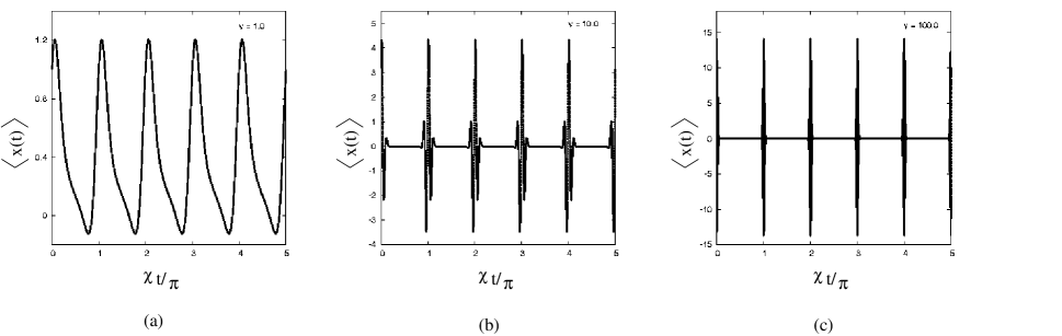
Figure 1: $\left\langle{x}\right\rangle$ as a function of time

Figures 1(a)-(c) show the variation of $\left\langle{x(t)}\right\rangle$ as a function of $t$ for small, medium and large values of $\nu$. (As already mentioned, $\left\langle{p(t)}\right\rangle$ displays similar behavior.) For sufficiently large values of $\nu$, it is evident that, except for times close to integer multiples of $T_{\rm rev}=\pi/\chi$, $\left\langle{x(t)}\right\rangle$ and $\left\langle{p(t)}\right\rangle$ essentially remain static at the value zero.

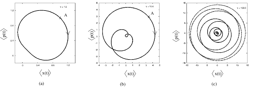
Figure 2: “Phase plot” of $\left\langle{p}\right\rangle$ versus $\left\langle{x}\right\rangle$

Figures 2(a)-(c) depict the corresponding “phase plots” in the $(\left\langle{x}\right\rangle,\left\langle{p}\right\rangle)$ plane. In Fig. 2(c), the representative point remains at the origin most of the time, except at times close to successive revivals, when it rapidly traverses the rest of the curve before returning to the origin.

While sudden changes from nearly static values of $\left\langle{x(t)}\right\rangle$ and $\left\langle{p(t)}\right\rangle$ are thus signatures of revivals, the occurrence of fractional revivals is not captured in these mean values. The fractional revival occurring mid-way between successive revivals (e.g., at $t=\pi/2\chi$ in the interval between $t=0$ and $t=T_{\rm rev}$), when the initial wave packet reconstitutes itself into two separate wave packets of a similar kind, leaves its signature upon the second moments. Figures 3(a)-(c) show the variation with time of the uncertainty product $\Delta x\,\Delta p$. In each case, this product returns to its initial, minimum value $\frac{1}{2}$ at every revival, rising to higher values in between revivals.

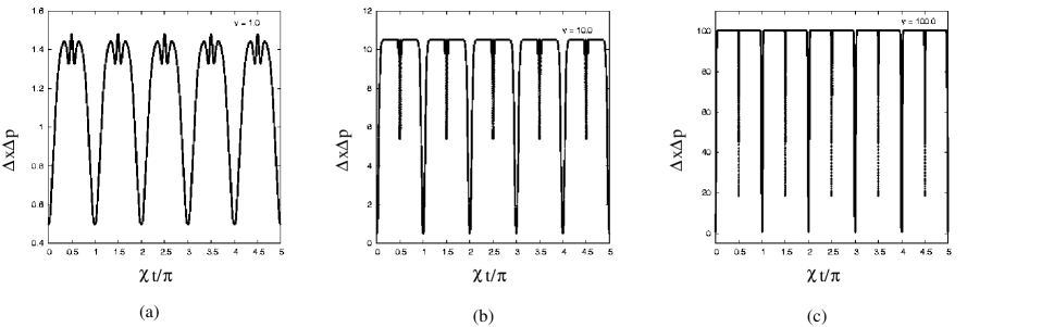
Figure 3: Variation of the uncertainty product with time

Once again, for sufficiently large values of $\nu$, the product remains essentially static at the approximate value $(\frac{1}{2}+\nu)$ for most of the time, but undergoes extremely rapid variation near revivals, and also near the fractional revivals occurring mid-way between revivals. During the latter, the uncertainty product drops to smaller values, but does not reach the minimum value $\frac{1}{2}$.

There is a very striking difference in the behavior of the standard deviations near revivals as opposed to their behavior near the foregoing fractional revivals. This is brought out in Figs. 4(a)-(c), which is a “phase plot” of $\Delta p$ versus $\Delta x$.

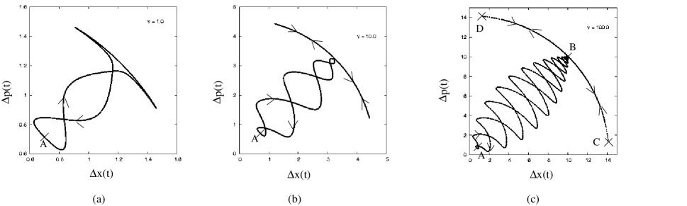
Figure 4: “Phase plot” of $\Delta p$ versus $\Delta x$

For very small $\nu$, as in Fig. 4(a), $\Delta x$ and $\Delta p$ vary quite gently around a simple closed curve. When $\nu$ is somewhat larger, as in 4(a) which corresponds to $\nu=1$, the plot begins to show interesting structure. For much larger values of $\nu$ as in 4(c), the initial point A quickly moves out on the zig-zag path about the radial $\Delta p=\Delta x$ line to the steady value represented by the point B, and returns to A at every revival along the complementary zig-zag path. Close to the fractional revival at $t=(n+\frac{1}{2})T_{\rm rev}$, however, the representative point moves back and forth along the azimuthal path BCDB rather than the zig-zag path: clearly, a kind of “squeezing” occurs, as one of the variances reaches a small value while the other becomes large, and vice versa. (Of course the state of the system is far from a minimum uncertainty state throughout, except at the instants $nT_{\rm rev}$.)

The fractional revivals occurring at $t=(n+\frac{1}{3})T_{\rm rev}$ and $t=(n+\frac{2}{3})T_{\rm rev}$, when the initial wave packet is reconstituted into a superposition of three separate wave packets, are detectable in the third moments of $x$ and $p$. To make this unambiguous, we may consider the third moments about the mean values — or, in standard statistical notation, the square of the skewness, defined as

$$\beta_{1}^{(x)}=\left\langle\big{(}x-\left\langle{x}\right\rangle\big{)}^{3}\right\rangle^{2}\Big{/}\big{(}\left\langle{x^{2}}\right\rangle-\left\langle{x}\right\rangle^{2}\big{)}^{3},$$ (19)

and similarly for $\beta_{1}^{(p)}$. Figures 5(a)-(c) show the variation of $\beta_{1}^{(x)}$ with $t$.

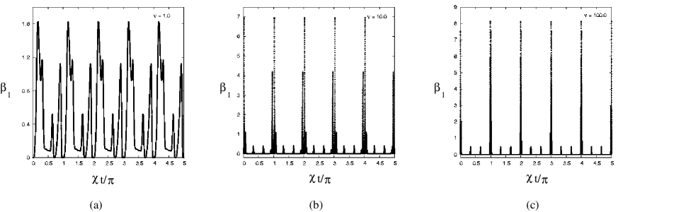
Figure 5: Square of the skewness in $x$ as a function of time

It is evident that, for sufficiently large values of $\nu$, $\beta_{1}^{(x)}$ remains nearly zero most of the time, except for bursts of rapid variation close to revivals and fractional revivals. Both $\beta_{1}^{(x)}$ and $\beta_{1}^{(p)}$ actually vanish at $t=nT_{\rm rev}$, but they remain non-zero at $t=(n+l/3)T_{\rm rev}\,,l=1,2$. More detailed information is obtained from a “phase plot” of $\beta_{1}^{(p)}$ versus $\beta_{1}^{(x)}$, which we do not give here.

Finally, we consider fractional revivals corresponding to $m=4$, when four superposed wave packets appear. These are detectable in the behavior of the fourth moments of $x$ and $p$. Equivalently, we may use the excess of kurtosis $(\beta_{2}-3)$, where the kurtosis of $x$ is defined as

$$\beta_{2}^{(x)}=\left\langle\big{(}x-\left\langle{x}\right\rangle\big{)}^{4}\right\rangle\Big{/}\big{(}\left\langle{x^{2}}\right\rangle-\left\langle{x}\right\rangle^{2}\big{)}^{2},$$ (20)

with a similar definition for $\beta_{2}^{(p)}$. The excess of kurtosis is the measure of the departure of a distribution from gaussianity. Figures 6(a)-(c) depict how $(\beta_{2}^{(x)}-3)$ varies with time.

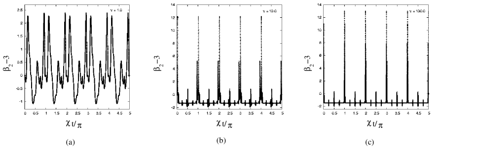
Figure 6: The excess of kurtosis of $x$ as a function of time

For sufficiently large $\nu$, both $(\beta_{2}^{(x)}-3)$ and $(\beta_{2}^{(p)}-3)$ remain essentially static near the value $-\frac{3}{2}$ for most of the time. They vary rapidly near revivals, vanishing at $t=n\,T_{\rm rev}$ because the wave packet is a Gaussian both in position space and in momentum space at these instants of time. As is clear from Fig. 4(c), they also vary rapidly near the fractional revivals at $t=(n+l/4)T_{\rm rev}\,({\rm where}\,l=1,2,3)$, oscillating about the “steady value” $-\frac{3}{2}$. Once again, a “phase plot” of $(\beta_{2}^{(p)}-3)$ versus $(\beta_{2}^{(x)}-3)$ (which we do not give here) helps identify features that distinguish between the three fractional revivals concerned.

We have shown that distinctive, experimentally detectable signatures of the different fractional revivals of a suitably prepared initial wave packet are displayed in the expectation values of physical observables and their powers. The complicated quantum interference effects that lead to fractional revivals can thus be captured in the dynamics of these expectation values, which may be regarded as the dynamical variables in a classical phase space. While this is, in principle, an infinite-dimensional space, what is relevant in practice is the temporal behavior of a finite number of moments, since fractional revivals corresponding to very large values of $m$ are not easy to detect in any case.

We thank Suresh Govindarajan for discussions and help. This work was supported in part by the Department of Science and Technology, India, under Project No. SP/S2/K-14/2000.

References

- (1) See for example, D. F. Walls, Nature (London) 280, 451 (1979); ibid. 306, 141 (1983).
- (2) P. D Drummond and D. F Walls, J. Phys. B 13, 725 (1980); M. Kitagawa and Y. Yamamoto, Phys. Rev. A 34 3974 (1986); A. Mecozzi and P. Tombesi, Phys. Rev. Lett. 58, 1055 (1987).
- (3) J. Parker and C. R. Stroud, Jr., Phys. Rev. Lett. 56, 716 (1986).
- (4) I. Sh. Averbukh and N. F. Perelman, Phys. Lett. A 139, 449 (1989); Acta Phys. Pol. A 78, 33 (1990).
- (5) Z. Dac̆ić Gaeta and C. R. Stroud Jr. Phys. Rev. A 42, 6308 (1990).
- (6) R. Bluhm and V. A Kostelecky, Phys. Rev. A 50, R4445 (1994); Phys. Lett. A 200, 308 (1995).
- (7) R. Bluhm and V. A Kostelecky, Phys. Rev. A 51, 4767 (1995).
- (8) J. Wals, H. H. Fielding, J. F. Christian, L. C. Snock, W. J. van der Zande and H. B. van Linden van den Heuvell, Phys. Rev. Lett. 72, 3783 (1994).
- (9) J. A. Yeazell and C. R. Stroud, Jr., Phys. Rev. A 43, 5153 (1991).
- (10) D. R Meacher, P. E. Meyler, I. G. Hughes and P. Evart, J. Phys. B 24, L63 (1991).
- (11) M. J. J. Vrakking, D. M. Villeneuve and A. Stolow, Phys. Rev. A 54, R37 (1996).
- (12) P. W. Dooley, I. V. Litvinyuk, K. F. Lee, D. M. Rayner, M. Spanner, D. M. Villeneuve and P. B Corkum, Phys. Rev. A 68, 023406 (2003).
- (13) R. W. Robinett, arXiv:quant-ph/0401031 (to appear in Physics Reports).
- (14) J. H. Eberly, N. R. Narozhny and J. J. Sanchez-Mondragon, Phys. Rev. Lett. 44, 1323 (1980); N. B. Narozhny, J. J Sanchez-Mondragon and J. H. Eberly, Phys. Rev. A 23, 236 (1981); H. I. Yoo and J. H. Eberly, Phys. Rep. 118, 239 (1985).
- (15) I. Sh. Averbukh, Phys. Rev. A 46, R2205 (1992).
- (16) P. Rozmej and R. Arvieu, Phys. Rev A 58, 4314 (1998).
- (17) J. Banerji and G. S. Agarwal, Phys. Rev A 59, 4777 (1999).
- (18) D. L. Aronstein and C. R. Stroud, Jr., Phys. Rev. A 55, 4526(1997).
- (19) C. Leichtle, I. Sh. Averbukh and W. P. Schleich, Phys. Rev. A 54, 5299 (1996).
- (20) B. Yurke and D. Stoler, Phys. Rev. Lett. 57, 13 (1986); G. J. Milburn and C. A. Holmes, ibid. 56, 2237 (1986); W. Schleich, M. Pernigo, and Fam le Kein, Phys. Rev. A 44, 2172 (1991); V. Buzek, H. Moya-Cessa and P. L. Knight, ibid. 45, 8190 (1992).
- (21) G. S. Agarwal and R. R Puri, Phys. Rev. A 39, 2969 (1989).
- (22) K. Tara, G.S Agarwal and S. Chaturvedi, Phys. Rev. A 47, 5024 (1993).
- (23) S. Seshadri, S. Lakshmibala and V. Balakrishnan, Phys. Lett. A 256, 15 (1999).
- (24) S. Seshadri, S. Lakshmibala and V. Balakrishnan, J. Stat. Phys. 101, 213 (2000).
- (25) R. Bluhm and V. A. Kostelecky, Phys. Rev. A 51, 4767 (1995).
- (26) O. Knospe and R. Schmidt, Phys. Rev. A 54, 1154 (1996).
- (27) P. A. Braun and V. G. Savichev, J. Phys. B: At. Mol. Opt. Phys. 29, L325 (1996).
- (28) P. A. Braun and V. G. Savichev, Phys. Rev. A 49, 1704 (1994).
- (29) M. Kitagawa and Y. Yamamoto, Phys. Rev. A 34, 3974 (1986).
- (30) M. Greiner, O. Mandel, T. W. Hänsch, and I. Bloch, Nature 419, 51 (2002).