Nonclassical imaging for a quantum search of trapped ions

Abstract

We discuss a simple search problem which can be pursued with different methods, either on a classical or on a quantum basis. The system is represented by a chain of trapped ions. The ion to be searched is a member of that chain, consists, however, of an isotopic species different to the others. It is shown that the classical imaging may lead as fast to the final result as the quantum imaging. However, for the discussed case the quantum method gives more flexibility and higher precision when the number of ions considered in the chain is increasing. In addition, interferences are observable even when the distances between the ions is smaller than half a wavelength of the incident light.

Quantum search algorithms grover enable us to determine an object from a black box with $N$ elements by a number of measurements which is of the order of $\sqrt{N}$. A quantum search thus provides a polynomial speed-up in comparison with any known classical algorithm. Several methods have been proposed for implementing a quantum search Chuang98 . In this letter we discuss a very simple example where the search can be performed in the same system either on a classical or a quantum basis. Such a situation is useful for illustrating the particular aspects of a quantum search with respect to a classical search. We recall that fluorescence imaging, i.e., measurement of the mean intensity of radiation scattered by atoms upon excitation, provides information about the density profile. In fact, this is a common method used to image, for example, trapped ions or a Bose-Einstein condensate Walther92 ; Blatt98 ; Ketterle00 . We could, however, do more than just image the sources of fluorescence, e.g. by determining the spectrum of the scattered light. In this case, in addition to the position the motional state of the atoms is accessible. Instead of imaging the particles individually on a detector, one could also observe the fluorescence in the far field or Fourier plane of a lens eichmann . In this case, the intensity distribution corresponds to the interference pattern described by the first order correlation function of the fluorescence light. It results from the contribution of all particles at once, and their relative position can be deduced from the interference pattern. The intensity distribution thus contains more information than the direct imaging of the ions grover2 . A further step in sophistication would be to observe the scattered light using two detectors and to measure the second order correlation function. This corresponds to a nonclassical imaging technique where the associated spatial distribution is determined by the different paths the photons can take when reaching the two detectors; the corresponding interference pattern again relies on the contribution of all scatterers simultaneously but for certain excitation angles is purely due to quantum interferences skornia01 ; agarwal02 . In this type of experiment only the coincidence events at the two detectors are recorded. As the paths of the photons contributing to these coincidences change with the relative position of the detectors and/or the scatterers, the observed interference patterns again allow the positions of the individual particles to be retraced. However, owing to the larger variability of the parameters involved, a much richer interference structure is obtained. To illustrate this in more detail we consider a particular example, viz. a linear chain of ions of the same atomic species. In order to set up a search procedure we assume that one of the ions belongs to an isotopic species different to the others. By calculating the spatial photon - photon correlations we then show how the second order correlations can be used to reveal information on the position of the off-resonant, non-radiating isotope in the chain. We will also demonstrate why this information is more extensive than that obtained from the usual fluorescence imaging techniques or first order correlation function. In particular, it will be shown that the second order correlation function is able to provide data in parameter regions where the first order correlation function is not able to provide any information.

Let us consider a chain of ions with an energy level scheme as shown in Fig. 1a. The transition $|g\rangle\rightarrow|e\rangle$ is used for exciting the system, whereas the transition $|e\rangle\rightarrow|f\rangle$ serves for fluorescence detection. The excitation could be performed, by for example, a short pulse of radiation. The most basic search protocol would consist in resonantly exciting each ion one by one on the $|g\rangle\rightarrow|e\rangle$ transition using a focused laser beam and observing the fluorescence scattered by the ion on the $|e\rangle\rightarrow|f\rangle$ transition. With the isotope being off-resonant and remaining dark upon excitation, it will take at most $N-1$ steps to localize the isotope, i.e. in the mean $N/2$ trials. One could next observe the fluorescence intensity in the far field or in the Fourier plane of a lens, i.e. without imaging the ions. The corresponding interference pattern - produced by the simultaneous superposition of the electromagnetic fields of all scatterers - can be used to extract information about the position of the isotope. To be explicit, let us calculate the far-field intensity produced by a chain of ions at some distance $r$. The positive frequency part of the field amplitude can be written as (see agarwalbook )

$$\vec{E}^{(+)}(\vec{r}_{1},t) = \vec{E}^{(+)}_{0}(\vec{r}_{1},t)$$

$$- \frac{k^{2}e^{ikr}}{r}\sum_{j}{\rm e}^{-ik\vec{n}_{1}\vec{R}_{j}}\vec{n}_{1}\times(\vec{n}_{1}\times\vec{d}_{fe})A^{(j)}_{fe},$$

where $\vec{n}_{1}$ stands for a unit vector in the direction of the detector position, $\vec{r}_{1}=\vec{n}_{1}r$, $k=\omega_{0}/c$. $\omega_{0}$, $\vec{d}_{fe}$ and $A^{(j)}_{fe}=|f\rangle_{jj}\langle e|$ are, respectively, the transition frequency, dipole matrix element and the dipole operator of ion $j$ for the transition $|e\rangle\rightarrow{|f\rangle}$ and the sum is over all ion positions $\vec{R}_{j}$ in the chain. The far-field intensity is thus determined by the first order correlation function $G^{(1)}(\vec{r}_{1})=\langle A^{\dagger}(\vec{r}_{1})A(\vec{r}_{1})\rangle$, where $A(\vec{r}_{1})=\sum_{j}A^{(j)}_{fe}{\rm e}^{-ik\vec{n}_{1}\vec{R}_{j}}$. In the case of uncorrelated ions ($\langle A^{(j)}_{ef}A^{(i)}_{fe}\rangle=\langle A^{(j)}_{ef}\rangle\langle A^{(i)}_{fe}\rangle$), $G^{(1)}(\vec{r}_{1})$ can be simplified to agarwalbook

$$G^{(1)}(\vec{r}_{1})=\sum_{j}\langle A^{(j)}_{ee}\rangle+\sum_{j\not=i}\langle A^{(j)}_{ef}\rangle\langle A^{(i)}_{fe}\rangle{\rm e}^{ik\vec{n}_{1}(\vec{R}_{i}-\vec{R}_{j})}.$$ (2)

According to (2), the information on the spatial structure of the ion chain is contained in $G^{(1)}(\vec{r}_{1})$ as long as $\langle A^{(j)}_{ef}\rangle\not=0$. This is the case as long as, for example, no $\pi$-pulse is used for the excitation. The information about the localization of a non-radiating particle is also contained in (2), as $G^{(1)}(\vec{r}_{1})$ will look different for different positions of the isotope. This will be discussed in more detail below. Note, however, that a result similar to (2) is obtained also in the case of classical dipoles or classical antennas, i.e. in the case of classical light sources grover2 .

As mentioned in the introduction, we could, however, do more than just measure the far-field intensity, e.g. by examining the quantum features of the emitted radiation. For that purpose let us study the spatial photon - photon correlations produced by the chain of ions by using two photodetectors (see Fig. 1b).

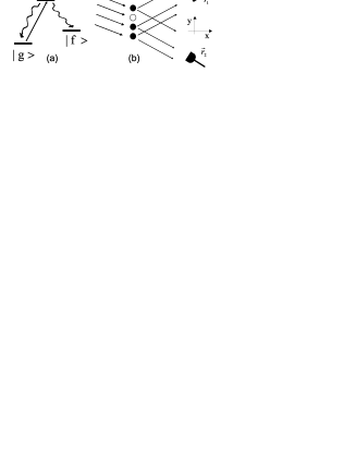
Figure 1: (a) Level scheme considered for the trapped ions: the ions are excited on the $|g\rangle\rightarrow|e\rangle$ transition, whereas the $|e\rangle\rightarrow|f\rangle$ transition is used for fluorescence detection; (b) an incident $\pi$-pulse of a wave with wave vector $\vec{k}_{L}$ excites the linearly trapped ions into their upper level $|e\rangle$. The fluorescence is then registered in the far field by two detectors at $\vec{r}_{i}$, $i=1,2$ ($|\vec{r}_{1}|=|\vec{r}_{2}|=r$).

The photon - photon correlations are determined by the expression (see agarwalbook )

$$\langle\vec{E}^{(-)}(\vec{r}_{1},t)\vec{E}^{(-)}(\vec{r}_{2},t)\vec{E}^{(+)}(\vec{r}_{2},t)\vec{E}^{(+)}(\vec{r}_{1},t)\rangle,$$ (3)

where $\vec{r}_{2}=\vec{n}_{2}r$ defines the position of the second detector and $\vec{E}^{(-)}(\vec{r}_{i},t)$ denotes the complex conjugate of $\vec{E}^{(+)}(\vec{r}_{i},t)$, $i=1,2$. As can be seen from (3), the spatial photon - photon correlations are determined in terms of the atomic/ionic operators through

$$G^{(2)}(\vec{r}_{1},\vec{r}_{2})=\langle A^{\dagger}(\vec{r}_{1})A^{\dagger}(\vec{r}_{2})A(\vec{r}_{2})A(\vec{r}_{1})\rangle.$$ (4)

In order to demonstrate how the information on the spatial structure of the chain is contained in the quantity $G^{(2)}(\vec{r}_{1},\vec{r}_{2})$, let us first examine the case of two ions. If the ions are initially prepared in the state $|e\rangle$, we find (see agarwal02 )

$$G^{(2)}(\vec{r}_{1},\vec{r}_{2})=B(1+\cos(k(\vec{n}_{2}-\vec{n}_{1})(\vec{R}_{A}-\vec{R}_{B}))),$$ (5)

where $B$ is a constant. Obviously, the information on the location of the two ions is contained in the nonclassical agarwal02 interference pattern $G^{(2)}(\vec{r}_{1},\vec{r}_{2})$ via the atomic position variables $\vec{R}_{A}$ and $\vec{R}_{B}$. Let us consider next a chain of $N$ ions of which one is an off-resonant, non-radiating isotope. The explicit calculation in case of $\pi$-excitation leads to the following result:

$$G^{(2)}_{p,N}(\vec{r}_{1},\vec{r}_{2})=\sum_{i,j\neq p(i<j)}|\gamma_{ij}(\vec{r}_{1},\vec{r}_{2})|^{2},$$ (6)

where $p=\overline{1,N}$ stands for the position of the isotope, $i=\overline{1,N-1}$ and $j=\overline{2,N}$ and $\gamma_{lm}(\vec{r}_{1},\vec{r}_{2})=\alpha_{l}(\vec{r}_{1})\beta_{m}(\vec{r}_{2})+\alpha_{m}(\vec{r}_{1})\beta_{l}(\vec{r}_{2})$ with $\alpha_{l}(\vec{r}_{1})={\rm e}^{ik{\vec{n}}_{1}{\vec{R}}_{l}}$ and $\beta_{m}(\vec{r}_{2})={\rm e}^{ik{\vec{n}}_{2}{\vec{R}}_{m}}$ ($l,m=\overline{1,N}$). The solution (6) can easily be interpreted as the sum of terms associated with all possible optical path differences between the photons when scattered by two different ions and recorded by the two detectors, on the assumption that the isotope at $p$ does not scatter at all. Equation (6) becomes even more transparent for equally spaced ions. In the case of four ions, for example, the system after initial excitation by a $\pi$-pulse will be in one of the pure states $|feee\rangle$, $|efee\rangle$, $|eefe\rangle$ or $|eeef\rangle$. In this case we get $|\gamma_{12}(\vec{r}_{1},\vec{r}_{2})|^{2}\equiv|\gamma_{23}(\vec{r}_{1},\vec{r}_{2})|^{2}\equiv|\gamma_{34}(\vec{r}_{1},\vec{r}_{2})|^{2}=2+2c_{1}(\vec{r}_{1},\vec{r}_{2})$ and $|\gamma_{13}(\vec{r}_{1},\vec{r}_{2})|^{2}\equiv|\gamma_{24}(\vec{r}_{1},\vec{r}_{2})|^{2}=2+2c_{2}(\vec{r}_{1},\vec{r}_{2})$, where $c_{m}(\vec{r}_{1},\vec{r}_{2})=\cos[k(\vec{n}_{1}-\vec{n}_{2})(\vec{R}_{1}-\vec{R}_{m+1})]$, so that

$$G^{(2)}_{p,4}(\vec{r}_{1},\vec{r}_{2})=$$ (7)

$$=2(\delta_{p,1}+\delta_{p,4})(3+2c_{1}(\vec{r}_{1},\vec{r}_{2})+c_{2}(\vec{r}_{1},\vec{r}_{2}))$$

$$+2(\delta_{p,2}+\delta_{p,3})(3+c_{1}(\vec{r}_{1},\vec{r}_{2})+c_{2}(\vec{r}_{1},\vec{r}_{2})+c_{3}(\vec{r}_{1},\vec{r}_{2})).$$

where $\delta_{p,q}$ is the Kronecker symbol.

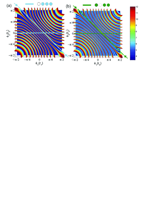
Figure 2: 3-D plot of the second order correlation function $G^{(2)}_{p,4}(\vec{r}_{1},\vec{r}_{2})$ versus the two detector positions $\phi_{i}(\vec{r}_{i}),$ $i=1,2$, for $N=4$ ions, with the off-resonant, non-radiating isotope placed in (a) the first (or fourth) position and (b) the second (or third) position of the chain. The distance between neighboring ions is $d=5.75\lambda$, wavelength of the incident light is $\lambda=194$nm and a $\pi$ pulse is used for the excitation.

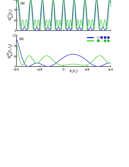
Figure 3: Interference patterns for $N=4$ ions. Blue and green curves correspond to the first (or fourth) and second (or third) ion being the isotope, respectively. Parameters are the same as in Fig. 2. (a) Classical interference pattern $G^{(1)}_{p,4}(\vec{r}_{1})$ (or second order correlation function $G^{(2)}_{p,4}(\vec{r}_{1},\vec{r}_{2})$ where the second detector is at $\phi_{2}(\vec{r}_{2})=0$). (b) Nonclassical interference pattern $G^{(2)}_{p,4}(\vec{r}_{1},\vec{r}_{2})$; the two detectors are slightly separated with $||\phi_{1}|-|\phi_{2}||=1/\pi$.

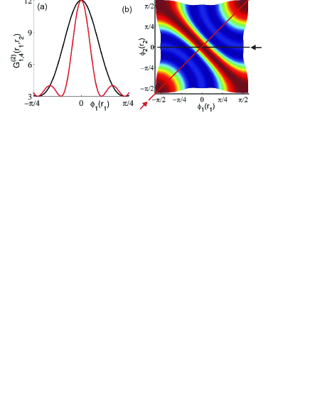
Figure 4: Interference patterns for $N=4$ ions with ion distance $\lambda/2$. (a) Red curve: nonclassical interference pattern $G^{(2)}_{1,4}(\vec{r}_{1},\vec{r}_{2})$ with $\phi_{1}(\vec{r}_{1})=\phi_{2}(\vec{r}_{2})$ (see red line in (b)), black curve: classical interference pattern $G^{(1)}_{1,4}(\vec{r}_{1})$ ($G^{(2)}_{1,4}(\vec{r}_{1},\vec{r}_{2})$ with $\phi_{2}(\vec{r}_{2})=0$; see black line in (b)).

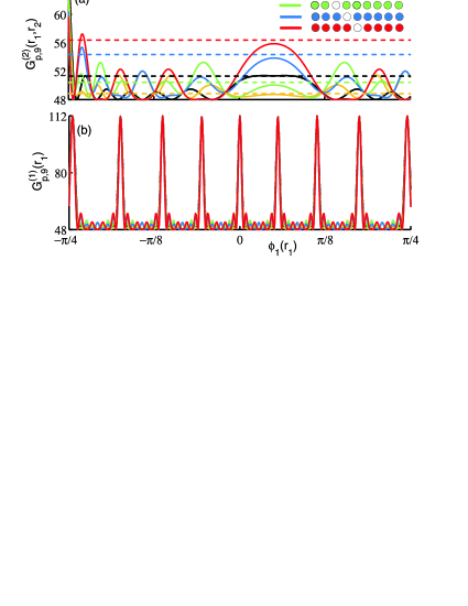
Figure 5: Interference patterns for $N=9$ ions. Black, yellow, green, blue and red curves correspond to 1st (or 9th), 2nd (or 8th), 3rd (or 7th), 4th (or 6th) and 5th ion being the isotope, respectively. Parameters are the same as in Fig. 2. (a) Nonclassical interference pattern $G^{(2)}_{p,9}(\vec{r}_{1},\vec{r}_{2})$; the two detectors have a constant separation $||\phi_{1}|-|\phi_{2}||=1/\pi$. Dashed lines correspond to detectors’ positions being chosen in such a way that $|sin|\phi_{1}|-sin|\phi_{2}||=0.378$. (b) Classical interference pattern $G^{(1)}_{p,9}(\vec{r}_{1})$.

According to (7), the information about the isotope position can be extracted from $G^{(2)}_{p,4}(\vec{r}_{1},\vec{r}_{2})$ due to the unique distribution of prefactors (or Fourier coefficients) $c_{j}$ for the different isotope localizations. From (7) it is seen, however, that the outcome for the isotope positions $p=1$ ($2$) is identical to the outcome for $p=4$ ($3$). This means that for equally spaced ions an additional measurement would be required to determine whether the isotope is on the left or right hand side with respect to the middle of the chain. A similar argument holds for the general outcome (6): for arbitrarily spaced ions there is a unique interference pattern for each isotope position $p$ since the $\gamma_{ij}$ will in general be different for different $i,j$, so that there is a unique combination of $\gamma_{ij}$ for each isotope position $p$. By measuring the spatial dependence of the photon-photon correlation function one could thus clearly distinguish the isotope position $p$ from any other position $p^{\prime}$. Note in particular that the additional degree of freedom given by $\vec{r}_{2}$ due to the use of two detectors increases the parameter space available. This is exceedingly useful when the information from the first order correlation function $G^{(1)}_{p,N}(\vec{r}_{1})$ is difficult to extract. This is the case for, for example, a large number of ions and/or a small ion spacing. There is in addition the particular situation where $G^{(1)}_{p,N}(\vec{r}_{1})$ contains no information at all, as is the case, for example, for a $\pi$-pulse excitation. In this case the contrast of the interference pattern of $G^{(1)}_{p,N}(\vec{r}_{1})$ vanishes, whereas that of $G^{(2)}_{p,N}(\vec{r}_{1},\vec{r}_{2})$ can still remain maximal skornia01 ; agarwal02 . In Fig. 2, we show the behavior in case of four equally spaced ions for $G^{(2)}_{p,4}(\vec{r}_{1},\vec{r}_{2})$ for $p=1$ (or $4$) and $p=2$ (or $3$) as a function of $\phi_{i}(\vec{r}_{i})=\arctan(r_{i,y}/r_{i,x})$, $i=1,2$. For the same excitation angle as used in this figure (i.e. $\pi$-pulse excitation) $G^{(1)}_{p,4}(\vec{r}_{1})$ would correspond to a constant, independently of $\phi_{1}(\vec{r}_{1})$ and independent of the isotope position $p$. For a $\pi/2$-pulse excitation on the $|f\rangle\rightarrow|e\rangle$ transition, however, $G^{(1)}_{p,4}(\vec{r}_{1})$ would - apart from a prefactor - show an interference pattern similar to $G^{(2)}_{p,4}(\vec{r}_{1},\vec{r}_{2})$ for $\pi$-pulse excitation and $\phi_{2}(\vec{r}_{2})=0$ (see horizontal lines in Fig. 2). More precisely, we obtain

$$G^{(1)}_{p,4}(\vec{r}_{1}) = 1/2(\delta_{p,1}+\delta_{p,4})(3+2c_{1}(\vec{r}_{1})+c_{2}(\vec{r}_{1}))$$

$$+ 1/2(\delta_{p,2}+\delta_{p,3})(3+c_{1}(\vec{r}_{1})+c_{2}(\vec{r}_{1})+c_{3}(\vec{r}_{1})).$$

where $c_{m}(\vec{r}_{1})=\cos[k\vec{n}_{1}(\vec{R}_{1}-\vec{R}_{m+1})]$ and $p=\overline{1,4}$. The result (up to a prefactor) is shown in Fig. 3a. Yet, it is here that the additional degree of freedom of $G^{(2)}_{p,4}(\vec{r}_{1},\vec{r}_{2})$ with respect to $G^{(1)}_{p,4}(\vec{r}_{1})$ becomes important: the additional parameter $\vec{r}_{2}$ increases the available parameter space and in this manner allows a more flexible and precise search of the isotope. To show that, we plot in Fig. 3b $G^{(2)}_{p,4}(\vec{r}_{1},\vec{r}_{2})$ for $p=1$ (or $4$) and $p=2$ (or $3$), and with $\vec{r}_{1}$ and $\vec{r}_{2}$ such that $||\phi_{1}(\vec{r}_{1})|-|\phi_{2}(\vec{r}_{2})||=1/\pi$. The latter condition stands for a fixed distance between the two detectors and corresponds in Fig. 2 to a straight line in the $(\phi_{1}(\vec{r}_{1}),\phi_{2}(\vec{r}_{2}))$-plane (see tilted lines in Fig. 2). As is seen from Fig. 3b, the constraints for the angular resolving power are much more relaxed in comparison with that needed for $G^{(1)}_{p,4}(\vec{r}_{1})$ (Fig. 3a).

The spatial second order correlation function also allows the isotope position to be determined in cases where the ions are separated by only $\lambda/2$ so that they cannot be individually resolved. This can be demonstrated by analyzing $G^{(2)}_{1,4}(\vec{r}_{1},\vec{r}_{2})$ for equally spaced ions with ion separation $d=\lambda/2$ (Fig. 4). If the detector positions are chosen such that $\phi_{1}(\vec{r}_{1})=\phi_{2}(\vec{r}_{2})$ - corresponding in the $(\phi_{1}(\vec{r}_{1}),\phi_{2}(\vec{r}_{2}))$-plane to a straight line with slope 1 - we resolve for $G^{(2)}_{1,4}(\vec{r}_{1},\vec{r}_{2})$ a central maximum plus two side maxima in the central region $-\pi/4\leq\phi_{1}(\vec{r}_{1})\leq\pi/4$, whereas for $G^{(1)}_{1,4}(\vec{r}_{1})$ only the central maximum is obtained (Fig. 4a). However, it is from the position and amplitude of the side maxima that the information about the isotope position $p$ is derived, whereas the central maximum in this regard contains no information.

Let us finally consider nine equally spaced ions in the trap one of which is an isotope. There are $5$ different positions for the isotope which can be distinguished from $G^{(2)}_{p,9}(\vec{r}_{1},\vec{r}_{2})$ (see above). These five different possibilities are plotted in Fig. 5a on the assumption that $||\phi_{1}(\vec{r}_{1})|-|\phi_{2}(\vec{r}_{2})||=1/\pi$ and a $\pi$-pulse is used for excitation. It can be clearly seen from the figure that the requirement for the angular resolving power is far less demanding in comparison with Fig. 5b, where $G^{(1)}_{p,9}(\vec{r}_{1})$ (apart from a prefactor) is plotted for a $\pi/2$-pulse excitation on the $|f\rangle\rightarrow|e\rangle$ transition. For a relative position of the two detectors such that $||\sin\phi_{1}(\vec{r}_{1})|-|\sin\phi_{2}(\vec{r}_{2})||=0.378$, one even obtains for $G^{(2)}_{p,9}(\vec{r}_{1},\vec{r}_{2})$ constant values, with amplitudes which depend on the isotope position $p$, but are independent from $\phi_{1}(\vec{r}_{1})$. These values are depicted in Fig. 5a by dashed lines. However, due to the nonlinear dependence of the two detector positions, this situation might be more difficult to implement experimentally. Nevertheless, such as special angular independent case could play an important role when one would be interested to normalize the correlation function, e.g. for the purpose of a better comparison between the different isotope positions.

In conclusion, it has been shown in a simple search problem using a chain of trapped ions that the search process can be strongly improved when interferences are observed than employing a one by one search. The speed up of the search process results from the fact that the interference patterns are produced by the light of all emitting ions of the chain at once so that there is a simultaneous contribution of all scatterers to the signal. This superposition of the signal is apparently sufficient for the speed up and no entanglement between the ions nor other quantum phenomena are required grover2 . However, quantum interferences allow to increase the parameter space available and in particular improve the precision when a larger number of ions is involved, since they relax the demands for the spatial resolving power of the detectors. Moreover, in the case of quantum interferences an interference pattern is obtained even at ion distances smaller than $\lambda/2$ which is the ultimate limit for a classical interference experiment.

Acknowledgement. One of the authors, (G.O.A.) gratefully acknowledges the support of the Alexander von Humboldt Foundation Fellowship.

References

- (1) L.K. Grover, Phys. Rev. Lett. 79, 325 (1997); M.O. Scully, M.S. Zubairy, Phys. Rev. A 64, 022304 (2001).
- (2) I.L. Chuang N. Gershenfeld, M. Kubinec, Phys. Rev. Lett. 80, 3408 (1998); I.L. Chuang, L.M.K. Vandersypen, X. Zhou, D.W. Leung, S. Lloyd, Nature 393, 143 (1998); J.A. Jones, M. Mosca, R.H. Hansen, ibid. 393, 344 (1998); M. Feng, Phys. Rev. A 63, 052308 (2001); F. Yamaguchi, P. Milman, M. Brune, J.M. Raimond, S. Haroche, ibid. 66, 010302 (2001); V.L. Ermakov, B.M. Fung, ibid. 66, 042310 (2002).
- (3) I. Waki, S. Kassner, G. Birkl, H. Walther, Phys. Rev. Lett. 68, 2007 (1992).
- (4) H.C. Nägerl, W. Bechter, J. Eschner, F. Schmidt-Kaler, R. Blatt, Appl. Phys. B 66, 603 (1998).
- (5) R. Onofrio, C. Raman, J.M. Vogels, J.R. Abo-Shaeer, A.P. Chikkatur, W. Ketterle, Phys. Rev. Lett. 85, 2228 (2000).
- (6) U. Eichmann, J. C. Bergquist, J. J. Bollinger, J. M. Gilligan, W. M. Itano, D. J. Wineland, M. G. Raizen, Phys. Rev. Lett. 70, 2359 (1993).
- (7) L.K. Grover, A. M. Sengupta, Phys. Rev. A 65, 032319 (2002); S. Lloyd, ibid. 61, 010301 (1999).
- (8) C. Skornia, J. von Zanthier, G.S. Agarwal, E. Werner, H. Walther, Phys. Rev. A 64, 063801 (2001).
- (9) G.S. Agarwal, J. von Zanthier, C. Skornia, H. Walther, Phys. Rev. A 65, 053826 (2002).
- (10) G.S. Agarwal, Quantum Optics, Springer Tracts in Modern Physics (Springer, Berlin, 1974), Vol. 70.