Nanosecond Dynamics of Single-Molecule Fluorescence Resonance Energy Transfer

Abstract

Motivated by recent experiments on photon statistics from individual dye pairs planted on biomolecules and coupled by fluorescence resonance energy transfer (FRET), we show here that the FRET dynamics can be modelled by Gaussian random processes with colored noise. Using Monte-Carlo numerical simulations, the photon intensity correlations from the FRET pairs are calculated, and are turned out to be very close to those observed in experiment. The proposed stochastic description of FRET is consistent with existing theories for microscopic dynamics of the biomolecule that carries the FRET coupled dye pairs.

Keywords: flourescence resonance energy transfer, single molecule, Ornstein-Uhlenbeck stochastic process, nanosecond dynamics, protein folding

1 Introduction

Recent significant advances in nano-technology make it possible to investigate molecular dynamics and structures at single-molecule level. Measurement of fluorescence resonant energy transfer (FRET) between a couple of dye molecules that are attached to complementary sites of a biomolecule like DNA or protein is particularly useful, because the sharply distance-dependent dipole-dipole interaction between the dye pair can serve as a ’spectroscopic ruler’ for the biomolecule [1, 2, 3]. FRET means a non-radiative quantum energy transfer from a donor that is a dye which initially absorbs light, to an acceptor which is another dye.

The FRET can be considered in the framework of the theory of Förster [1]. An input laser light excites the donor, whose one of decay channels is to migrate its excitation energy to the acceptor via dipole-dipole interaction. The energy transfer typically finishes within nanoseconds. The requirements for FRET to occur efficiently are, at least, one of the chromophores should have a sufficient quantum yield and the donor fluorescence spectrum must overlap the acceptor absorption spectrum.

Photon-photon correlations associated with the chromophores contain information on the conformational distance of the biomolecule. Such information is usually washed out in traditional ensemble measurement, but is readily available in single-molecular measurement. Recently, using a Hanbury-Brown–Twiss [4] time-interval apparatus, Berglund et al. [5] have measured photon intensity correlations for individual donor-acceptor pairs on DNA. To interpret the experimental data, they proposed a dual FRET model. A continuous model emphasizing overall conformational change of the biomolecule has also been studied by several authors [6, 7]. However, it is important to note that there exists non-trivial interplay between biomolecular diffusion, which under physiological conditions can change drastically the molecular conformation over nanoseconds, and the quantum optical processes of a pair of FRET coupled dyes, which are also of the time scale of nanoseconds. In this paper, we show that the laser-induced FRET dynamics can be modelled by the stochastic Ornstein–Uhlenbeck (OU) process [8]. The underlying stochastic process is a Gaussian random process [9] with finite correlation time. The density matrix equations acquire the character of stochastic differential equations which can be solved using well-established methods. We shall demonstrate that the OU process is a good approximation to the FRET dynamics as measured on biomolecules. This paper is organized as follows. In section 2 we present our theoretical model of FRET. The idea of modelling FRET dynamics as an OU stochastic process is further elucidated in the context of biomolecular dynamics in solution. In section 3 and 4 we present the results of Monte-Carlo simulations and compare them with the experimental work.

2 Theory

In order to calculate the photon-photon correlation functions, we adopt a master equation approach. To derive the master equation for the system with two molecules coupled by FRET, we assume that the coherence time is much shorter than the time scale of experiments. We further note that a FRET coupled system is not a cascaded quantum system [10], i.e., to obtain an equation for only donor variables, after tracing over the acceptor variables from the general master equation, is impossible. The master equation for the density operator $\hat{\varrho}$, for the donor-acceptor pair couples four possible states $|q\rangle_{1}\otimes|p\rangle_{2}$ here $q=0,1$ ($p=0,1$) stands for the ground and excited states of the donor (acceptor) [5]:

$$\frac{d\hat{\varrho}}{dt}=\sum_{m=1}^{5}\Gamma_{m}(t)\left\{\hat{\Gamma}_{m}\hat{\varrho}\hat{\Gamma}_{m}^{\dagger}-\frac{1}{2}\left(\hat{\Gamma}_{m}^{\dagger}\hat{\Gamma}_{m}\hat{\varrho}+\hat{\varrho}\hat{\Gamma}_{m}^{\dagger}\hat{\Gamma}_{m}\right)\right\}$$ (1)

where $\Gamma_{m},m=1-5$ are rate coefficients for the dominant processes: spontaneous emissions of the donor and acceptor are described by the quantum jump operators $\hat{\Gamma}_{1}=\hat{\sigma}_{1}\otimes\hat{1}_{2}$ and $\hat{\Gamma}_{2}=\hat{1}_{1}\otimes\hat{\sigma}_{2}$; laser excitations of the donor and acceptor by $\hat{\Gamma}_{3}=\hat{\sigma}_{1}^{+}\otimes\hat{1}_{2}$ and $\hat{\Gamma}_{4}=\hat{1}_{1}\otimes\hat{\sigma}_{2}^{+}$; and transfer of energy from the donor to the acceptor by $\hat{\Gamma}_{5}=\hat{\sigma}_{1}\otimes\hat{\sigma}_{2}^{+}$. Here $\hat{\sigma}_{i}$ ($\hat{\sigma}_{i}^{+}$) is the lowering (raising) operator between the excited and the ground states for the $i$th dye molecule ($i=1$ for the donor and 2 for the acceptor). The master equation (1) ignores all coherence effects as they play no important role in FRET. The conditional photon count probability of the donor-acceptor system within a time delay $\tau$ can be represented as a normally ordered correlation function [10]

$$\langle:\hat{I}_{i}(t+\tau)\hat{I}_{j}(t):\rangle={\rm Tr}_{i,j}\left\{\hat{\sigma}_{i}^{+}\hat{\sigma}_{i}\hat{V}(\tau)\left\{\hat{\sigma}_{j}\hat{\varrho}(t)\hat{\sigma}_{j}^{+}\right\}\right\}$$ (2)

here $\hat{\varrho}(t)$ is the stationary operator solution of Eq. (1), and $\hat{V}(\tau)$ is the evolution operator of the whole system satisfying $\hat{V}(\tau)\hat{\varrho}(t)=\hat{\varrho}(t+\tau)$.

FRET measurements provide us information about dipole-dipole coupling, which varies as $1/{r^{3}}$ [11]. The FRET rate coefficient is given by

$$\Gamma_{5}(t)=\Gamma_{1}\left(\frac{R_{0}}{r(t)}\right)^{6}$$ (3)

where $R_{0}$ is the Förster radius, $r(t)=|{\bf r}_{1}(t)-{\bf r}_{2}(t)|$ is the distance between two chromophores. Considering intra-chain diffusion of a biomolecule, e.g., a protein molecule that carries the donor and the acceptor at a couple of complementary sites, the displacement of the donor-acceptor distance from its fixed (or initial) value, $x(t)=r(t)-r(0)$, can be modelled as a Brownian motion in a harmonic potential. Since a biomolecule which consists of a large number of atoms and molecules, we essentially deal with the over-damped regime, where the Brownian motion is described by the Langevin equation [9]

$$\frac{\partial x(t)}{\partial t}=-\lambda x(t)+\lambda f_{x}(t)$$ (4)

where $\lambda=\omega^{2}/\eta$ with $\omega$ being the frequency of harmonic oscillator, and $\eta$ the friction coefficient. The random force $f_{x}(t)$ is a pure Gaussian characterized by $\langle f_{x}(t)\rangle=0$ and $\langle f_{x}(t)f_{x}(t+t^{\prime})\rangle=2\theta\delta(t-t^{\prime})$. The solution of the Langevin equation, $x(t)$, resembles a white noise: its equilibrium distribution is

$$\rho^{eq}(x)=\frac{1}{\sqrt{2\pi\theta\lambda}}{\rm exp}\left(-\frac{x^{2}}{2\theta\lambda}\right).$$ (5)

and the correlation is

$$\langle x(t)x(t^{\prime})\rangle=\theta\lambda e^{-\lambda|t-t^{\prime}|}.$$ (6)

Now turn to the FRET rate Eq. (3), which can be rewritten as $\Gamma_{5}(t)=\Gamma_{5}(0)/[1+x(t)/r(0)]^{6}$ with $\Gamma_{5}(0)=\Gamma_{1}[R_{0}/r(0)]^{6}$ corresponding to the FRET rate at some fixed interdye distance. If the displacement $x$ is small as compared to $r(0)$, then we have

$$\delta\Gamma_{5}(t)\sim x(t).$$ (7)

This is a possible interplay between the diffusion process and the FRET dynamics, although neither they are completely uncorrelated nor fully correlated. It turns out that a variance (i.e., ‘noise’) of the FRET rate has the statistical signature of a white noise. A sign such as ’noise of the noise’ usually leads to colored noise in the OU stochastic dynamics. Eq.(7) is a linearized approximate relation. Although, some dynamic details can not be seen for large variations, analytically, the exact numerical simulation may be done. This rather involved and so we have tried to produce reasonable results by retaining the leading term. This captures the physics reasonably well. Note that the OU stochastic process is stationary. Thus Eq.(1) becomes a stochastic differential equation as $\Gamma_{5}(t)=\Gamma_{5}(0)+\xi(t)$. We assume that $\xi(t)$ is a colored noise, which is described by the Langevin equation [12]

$$\frac{d}{dt}\xi=-\lambda\xi+\lambda\eta(t)$$ (8)

where time averages of white noise should be $\overline{\eta(t)}=0$ and $\overline{\eta(t)\eta(t^{\prime})}=2D\delta(t-t^{\prime})$. As well known the Eq. (8), yields the steady state correlation function

$$\left\{\overline{\xi(t)\xi(t^{\prime})}\right\}=D\lambda{\rm e}^{-\lambda|t-t^{\prime}|}$$ (9)

with $\overline{\xi(t)}=0$ and $\{...\}$ denotes the stochastic average over the initial conditions [13]. A parameter $D$ might be proportional to the diffusion coefficient $\theta$ and $\lambda$ is the same in Eq.(6) and Eq.(9). The stochastic differential equation Eq.(1) will be solved using Monte-Carlo numerical simulations. A Box-Mueller algorithm and the Euler-Maruyama method have been used to realize the colored noise. Moreover, by virtue of an integral algorithm developed in [13], we have verified that the Monte-Carlo generated correlation fits perfectly to its analytical expression Eq. (9). To achieve this, a stochastic averaging over as large as $1000$ realizations is essential [14]. It must be borne in mind that the FRET rate is always positive which is done by keeping a background constant value $\Gamma_{5}(0)$. However, some large negative random numbers have to be omitted. To prove that these omitted random numbers do not play important role, we have also calculated the correlation for $\Gamma_{5}(t)$ which decreases exponentially as given in Eq.(9). Namely, we assume that $\Gamma_{H}\geq\Gamma_{5}(t)\geq\Gamma_{L}$ where the FRET rate is finite. $\Gamma_{H}$ ($\Gamma_{L}$) corresponds to minimum (maximum) inter-dye distance due to continues intrachain diffusion of the protein molecule. The quantities are determined by contour length and bending rigidity of the protein. In our case, we have assumed that the FRET does not occur between distant dyes, so that $\Gamma_{L}=0$. We take also $\Gamma_{H}=max(\Gamma_{5}(t))$ as a maximum value of the generated random numbers.

3 Results and discussions

Using Monte-Carlo simulations we have calculated correlation functions as defined in Eq. (2). In Fig. 1 we present the results for the normalized correlations $g^{(2)}_{ij}(\tau)$ defined by

$$g^{(2)}_{ij}(\tau)=\frac{\langle:\hat{I}_{i}(t+\tau)\hat{I}_{j}(t):\rangle}{\langle:\hat{I}_{i}(t)\hat{I}_{j}(t):\rangle}.$$ (10)

Since only two parameters, $D$ and $\lambda$, are needed to completely specify an OU process, their determination would be a desired contact between theory and experiment. As we see in Fig. 1, the normalized correlation functions are very similar to those observed in the experiment[5]. For the data shown in Fig. 1 the correlation time is taken to be $\tau_{c}=1/\lambda=7$. In this case we take the parameter $\Gamma_{5}(0)$ to be $0.65$ in order to ensure that the average FRET coefficient to be around $1$. The FRET coefficients fluctuate between $\Gamma_{L}=0$ and $\Gamma_{H}=5$. The estimated Förster radius, for instance, for the TMR-Cy5 dye pair that is frequently used in biomolecular measurement, is about $53$ Å [2]. Given the calculated average FRET coefficient of $1$, the average distance would be approximately $50$ Å. Intensity autocorrelations show the typical quantum feature of antibunching that is characteristic of emissions from individual dye molecules. Following the initial photon antibunching, photon bunching appears in the acceptor autocorrelation function. A sufficient stochastic deviation from its equilibrium distribution of the FRET rate is the hallmark of the generation of photon bunching, which is a tendency for clustered emissions. For large $\tau$ the normalized correlation functions go to unity indicating uncorrelated emissions. The appearance of the photon bunching in the donor autocorrelation was first predicted theoretically by Haas and Steinberg [6]. A pronounced antibunching associated with a photon blockade effect and a photon bunching in the cross talk of the acceptor-donor pair, for short time, has also been discussed in [5]. We also notice in the experimental results that over longer times, photons emitted by the donor are becoming correlated with photons emitted by the acceptor and vice versa. It is also worth noting that because of off-resonant excitation of the acceptor, the corresponding rate for the acceptor is as small as $f\Gamma_{3}$ with $f=0.1$. Otherwise, the acceptor would have already been excited by the laser, and FRET may not occur. For the same reason the laser excitation rate should not be too large. The bunching signal can be described approximately by an exponential $y=1+Ce^{-\lambda_{0}\tau}$, with the fitting parameter $\lambda_{0}$ proportional to $\lambda$. The tail of exponential decay, especially in the acceptor autocorrelation function is determined by the correlation time $\tau_{c}$ of the OU process. It is obvious that a larger value of the correlation time results in a longer tail. While being supported by the simulation results (Fig. 1), this point can be made clearer by assuming that the intra-chain diffusion of the biomolecule that carries the dyes, and thereby fluctuation of the donor-acceptor distance is much slower than the quantum optical process of the donor and acceptor. The population on the excited states then adiabatically follows the slowly varying $\Gamma_{5}(t)$, so that the intensity of the acceptor can be approximated as[7]

$$I_{2}(t)=\Gamma_{3}\left(f+\frac{\Gamma_{5}(r(t))}{\Gamma_{5}(r(t))+\Gamma_{1}}\right).$$ (11)

According to this adiabatic approximation in longer time delay $\tau$, the intensity correlation is an exponential [7]

$$g_{22}^{(2)}(\tau)\simeq 1+\frac{(I_{H}-I_{L})^{2}}{(I_{H}+I_{L})^{2}}e^{-2t/\tau}$$ (12)

where we have assumed that the dual FRET rates result in a high value and a low value of the emission intensity, $I_{H}$ and $I_{L}$, respectively. Using $\Gamma_{H}=5$ and $\Gamma_{L}=0$ obtained in the calculation for Fig. 1, we find that $I_{H}=0.93$ and $I_{L}=0.1$ from Eq.(11). The correlation function under the adiabatic approximation given by Eq.(12) has been also plotted, see the dotted curve in Fig. 1.

4 Conclusions

We have shown how the FRET process as measured for biomolecules in solution can be modelled using the Ornstein-Uhlenbeck stochastic theory. This theory predicts the fluorescence intensity correlations from the FRET coupled dye pair, which are very similar to those observed in recent experiments. An analytic study based on the local linearization procedure also shows that it is consistent with existing theory for microscopic dynamics of the biomolecule that carries the FRET coupled dye pairs. The second-order intensity correlation functions for a FRET coupled dye pair, are largely determined by only a few statistical parameters of the FRET dynamics. It is found that the stochastic OU description helps elucidate the underlying mechanism for the experimentally observed fluorescence correlations that typically exhibit exponential decay over nanosecond timescale.

Acknowledgement. This work was supported by ONR grant N00014-03-1-0639 and N00014-02-1-0741; Welch Foundation grant A-1261; AFRL grant F30602-01-1-0594 and TITF. One of us, (G.O.A.) also acknowledges the support of the Humboldt Foundation Fellowship.

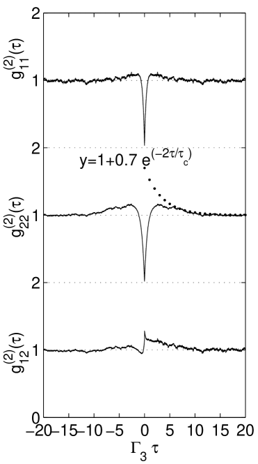
Figure 1: Normalized photon-photon correlation functions corresponding to donor-donor, acceptor-acceptor and donor-acceptor emissions. The parameters of the model (1) are chosen as $\Gamma_{1,2,3}=1,\Gamma_{4}=0.1,\Gamma_{5}(0)=0.65,\ (\overline{\Gamma_{5}(t)}\simeq 1,\ 0\leq\Gamma_{5}(t)\leq 5)$. The noise parameters are taken as $\tau_{c}=1/\lambda=7$ and $D=7$. The number of numerical realizations and a time step are taken to be $N=1000$ and $dt=0.01$, respectively.

References

- [1] T. Förster, Ann. Phys. 2, 55 (1948).
- [2] A.A. Deniz et al., Proc. Natl. Acad. Sci. U.S.A. 96, 3670 (1999).
- [3] E.A. Lipman, B. Schuler, O. Bakajin and W.A. Eaton, Science 301, 1233 (2003)
- [4] M.O. Scully and M.S. Zubairy Quantum Optics (Cambridge University Press, U.K., 1997).
- [5] A.J. Berglund, A.C. Doherty and H.Mabuchi, Phys. Rev. Lett. 89, 068101 (2002).
- [6] E. Haas and I.Z. Steinberg, Biophys. J. 46 429 (1984).
- [7] Z. Wang and D.E. Makarov, J. Phys. Chem. B107, 5617 (2003).
- [8] G.E. Uhlenbeck and L.S. Ornstein, in Selected Papers on Noise and Stochastic Processes ed. N. Wax, (Dover Publications, INC., New York, U.S.A., 1954), p823.
- [9] N. G. van Kampen, Stochastic Processes in physics and chemistry (North Holland, 1981).
- [10] C. W. Gardiner and P. Zoller, Quantum Noise: a Handbook of Markovian and Non-Markovian Quantum Stochastic Mehtod with Applications to Quantum Optics (Springer, Berlin, 2000).
- [11] G.S. Agarwal, Quantum Optics: Quantum Statistical Theories of Spontaneous Emission and Their Relation to Other Approaches (Springer-Verlag, Berlin, 1974).
- [12] W.T. Coffey, Yu.P. Kalmykov and J.T. Waldron, The Langevin Equation with Application in Physics, Chemistry and Electrical Engineering (World Scientific, Singapore, 1996).
- [13] R.F. Fox, I.R. Gatland, R. Roy and G. Vemuri, Phys. Rev. A 38, 5938 (1988).
- [14] G. Vemuri and G.S. Agarwal, Phys. Rev. A 42, 1687 (1990), G. Vemuri, R. Roy and G.S. Agarwal, ibid. 41, 2749 (1990).