Quantum freeze of fidelity decay for chaotic dynamics

Abstract

We show that the mechanism of quantum freeze of fidelity decay for perturbations with zero time-average, recently discovered for a specific case of integrable dynamics [New J. Phys. 5 (2003) 109], can be generalized to arbitrary quantum dynamics. We work out explicitly the case of chaotic classical counterpart, for which we find semi-classical expressions for the value and the range of the plateau of fidelity. After the plateau ends, we find explicit expressions for the asymptotic decay, which can be exponential or Gaussian depending on the ratio of the Heisenberg time to the decay time. Arbitrary initial states can be considered, e.g. we discuss coherent states and random states.

The question of stability of quantum time evolution with respect to small changes in the Hamiltonian has recently attracted lot of attention fidelity ; jalabert . This question is particularly important in the context of quantum information processing qcomp . The central quantity for describing quantum stability is the fidelity $F(t)=|\langle\psi(t)|\psi_{\delta}(t)\rangle|^{2}$ where $|\psi(t)\rangle=U_{0}(t)|\psi\rangle$ and $|\psi_{\delta}(t)\rangle=U_{\delta}(t)|\psi\rangle$ are unperturbed and perturbed time evolutions, of perturbation strength $\delta$, respectively, starting from the same initial state $|\psi\rangle$. Let the evolution operator be written as time-ordered product $U_{\delta}(t)={\cal\hat{T}}\exp(-{\rm i}\int_{0}^{t}{\rm d}t^{\prime}H_{\delta}(t^{\prime})/\hbar)$ in terms of (generally time-dependent) Hamiltonian $H_{\delta}(t)=H_{0}(t)+\delta H^{\prime}(t)$. In this Letter we either assume that $H_{\delta}(t)$ is autonomous (time-independent), or more generally, periodically time dependent with some period $\tau$, $H_{\delta}(t+\tau)=H_{\delta}(t)$. Then the time is measured in discrete units of $\tau$, namely $t=n\tau$, and the former (autonomous) case is simply obtained as the limit $\tau\to 0$. The perturbed propagator for one time step can be written as $U_{\delta}(\tau)=U_{0}(\tau)\exp(-{\rm i}V\tau\delta/\hbar)$ in terms of a hermitean perturbation $V$ which in the leading order perturbs the Hamiltonian $V=H^{\prime}+{\cal O}(\tau\delta)$.

It has been shown jalabert that for classically chaotic systems and for sufficiently strong perturbation and coherent initial state $|\psi\rangle$ the fidelity decay is given by classical Lyapunov exponents, and this phenomenon has been recently explained solely on the basis of classical dynamics VP . On the other hand, for sufficiently small $\delta$, one can express fidelity decay in terms of a power series in $\delta$ where coefficients are given as time-correlation function of the perturbation PZ . Using this approach one can derive universal forms of fidelity decay in both cases of classically regular and chaotic dynamics and express all time-scales solely in terms of classical quantities and $\hbar$.

The starting point of our analysis is the representation of fidelity $F^{(n)}=F(n\tau)$ in terms of expectation value PZ

$$F^{(n)}=|f^{(n)}|^{2},\quad f^{(n)}=\langle\psi|M_{\delta}^{(n)}|\psi\rangle$$ (1)

of the echo operator $M_{\delta}^{(n)}:=U_{0}(-n\tau)U_{\delta}(n\tau)$ which is the propagator in the interaction picture. Namely

$$M_{\delta}^{(n)}={\cal\hat{T}}\exp\left(-{\rm i}\frac{\delta}{\hbar}\Sigma_{n}(V)\right),$$ (2)

where, for any operator $A$, $\Sigma_{n}(A):=\tau\sum_{n^{\prime}=0}^{n-1}A_{n^{\prime}}$ and $A_{n}:=U_{0}(-n\tau)AU_{0}(n\tau)$. In case of continuous time: $M_{\delta}(t)={\cal\hat{T}}\exp(-{\rm i}\frac{\delta}{\hbar}\Sigma(V,t))$, with $\Sigma(A,t):=\int_{0}^{t}{\rm d}t^{\prime}A(t^{\prime})$, $A(t):=U_{0}(-t)AU_{0}(t)$. Approach PZ using the power law expansion of (2) in $\delta$ gives to the second order

$$F^{(n)}=1-\frac{\delta^{2}}{\hbar^{2}}\left\{\left\langle\Sigma^{2}_{n}(V)\right\rangle-\left\langle\Sigma_{n}(V)\right\rangle^{2}\right\}+{\cal O}(\delta^{4})$$ (3)

where $\left\langle\bullet\right\rangle:=\langle\psi|\bullet|\psi\rangle$. Equivalently, this useful formula can be expressed in terms of time-correlation function $C(n^{\prime},n^{\prime\prime})=\left\langle V_{n^{\prime}}V_{n^{\prime\prime}}\right\rangle-\left\langle V_{n^{\prime}}\right\rangle\left\langle V_{n^{\prime\prime}}\right\rangle$, namely $F^{(n)}=1-(\tau\delta/\hbar)^{2}\sum_{n^{\prime},n^{\prime\prime}=0}^{n-1}C(n^{\prime},n^{\prime\prime})+\ldots$ The rule of thumb says that slower decay of correlations, i.e. stronger fluctuation of $\Sigma_{n}(V)$, imply faster decay of fidelity, and vice versa.

Particularly interesting special situation arises when a time averaged perturbation $\bar{V}:=\lim_{n\to\infty}(n\tau)^{-1}\Sigma_{n}(V)$ equals zero. In general, the perturbation can be decomposed into the diagonal and residual part $V=\bar{V}+V_{\rm res}$. The part $\bar{V}$ which commutes with the unperturbed evolution $U_{0}$ and is thus diagonal in its eigenbasis can sometimes be put together with the unperturbed Hamiltonian $H_{0}$. This is customary in various quantum mean field approaches. It is thus interesting to question the stability of quantum dynamics with respect to residual perturbation only (i.e. when its diagonal part exactly vanishes $\bar{V}=0$). This problem has been addressed for the particular case of perturbed integrable dynamics ifreeze and very interesting results on extreme stability of quantum dynamics have been found termed as ’quantum freeze of fidelity’.

In this Letter we show that the phenomenon of quantum freeze, namely the saturation of fidelity to a plateau of high value, is much more general and robust as it appears in Ref.ifreeze , and applies to arbitrary quantum evolution provided only that the perturbation is residual, $\bar{V}=0$. In particular, we work out in detail the important case of dynamics with fully chaotic classical counterpart. We compute the plateau value (scaling as $1-{\rm const}\delta^{2}$ within the second order), its range scaling as $1/\delta$, and the rate of the asymptotic decay after the plateau ends (which is either gaussian or exponential), quantitatively in terms of the underlying classical dynamics, effective perturbation $\delta$ and the effective value of Planck constant $\hbar$. The phenomenon may find useful application in quantum computation where fidelity error is predicted to be very small and frozen in time (for sufficiently small $\delta$) provided only that the diagonal part of the error in each gate can be cured by some other means.

In the autonomous case ($\tau\to 0$), provided that the spectrum of $H_{0}$ is non-degenerate (which is true for a generic non-integrable system), the perturbation is residual iff it can be written as a time derivative of some observable $W$ i.e. a commutator with $H_{0}$, $V=\frac{{\rm i}}{\hbar}[H_{0},W]=(d/dt)W$. Generalizing to the discrete, time-periodic case we shall assume that the perturbation is of the form

$$V=\frac{1}{\tau}\left(W_{1}-W_{0}\right)=\frac{1}{\tau}\left(U_{0}(-\tau)WU_{0}(\tau)-W\right).$$ (4)

We shall now apply the Baker-Campbell-Hausdorff expansion $e^{A}e^{B}=\exp(A+B+(1/2)[A,B]+\ldots)$ to the time-ordered product (2) and rewrite the echo-operator

$$M^{(n)}_{\delta}=\exp\left\{-\frac{{\rm i}}{\hbar}\left(\Sigma_{n}(V)\delta+\frac{1}{2}\Gamma_{n}\delta^{2}+\ldots\right)\right\}$$ (5)

where $\Gamma_{n}:=\frac{{\rm i}\tau^{2}}{\hbar}\sum_{n^{\prime}=0}^{n-1}\sum_{n^{\prime\prime}=n^{\prime}}^{n-1}[V_{n^{\prime}},V_{n^{\prime\prime}}]$. It is interesting to note ifreeze that all matrix elements of $\Gamma_{n}$ grow with $n$ not faster than $\propto n$ control . This becomes obvious for the special form of perturbation (4) for which it follows

$$\Sigma_{n}(V) = W_{n}-W_{0},$$ (6)

$$\Gamma_{n} = \Sigma_{n}(R)-\frac{{\rm i}}{\hbar}[W_{0},W_{n}],\quad R:=\frac{{\rm i}}{\tau\hbar}[W_{0},W_{1}],\qquad$$ (7)

so the operator $\Gamma_{n}$ is also a time sum/integral of a time-dependent operator $R$, minus a sort of time-correlation function which shall be neglected for systems with strong decay of correlations studied below. In the continuous time case, $R=\frac{{\rm i}}{\hbar}[W,(d/dt)W]=\hbar^{-2}[W,[W,H_{0}]]$ and $\Gamma(t)=\int_{0}^{t}{\rm d}t^{\prime}R(t^{\prime})-\frac{{\rm i}}{\hbar}[W(0),W(t)]$. We note that, provided $W$ has a well defined classical limit $\hbar\to 0$, then also $V$, $R$ and $\Gamma_{n}$ have well defined limits since $\frac{{\rm i}}{\hbar}[\bullet,\bullet]$ can be replaced by a Poisson bracket. This is what we shall assume below, as well as that the limiting classical dynamics of $U_{0}$ is fully chaotic.

Comparing the two terms in the BCH exponential (5) we note that there should exist a time-scale $t_{2}\sim\delta^{-1}$, such that if $n\tau<t_{2}$ then the first term $\Sigma_{n}\delta$ dominates the second one $\frac{1}{2}\Gamma_{n}\delta^{2}$ (and higher control ). So, let us first consider the case $n\tau<t_{2}$. Then we can neglect the second term and write the fidelity amplitude

$$f^{(n)}=\left\langle\exp\left(-{\rm i}(W_{n}-W_{0})\delta/\hbar\right)\right\rangle.$$ (8)

Expanding $f^{(n)}$ to the second order in $\delta$, we find $F^{(n)}=1-\frac{\delta^{2}}{\hbar^{2}}(\kappa_{0}^{2}+\kappa_{n}^{2}-C_{n}-C_{n}^{*})$ where $\kappa_{k}^{2}:=\left\langle W_{k}^{2}\right\rangle-\left\langle W_{k}\right\rangle^{2}$, $C_{n}:=\left\langle W_{n}W_{0}\right\rangle-\left\langle W_{n}\right\rangle\left\langle W_{0}\right\rangle$. Using Cauchy-Schwartz inequality $|C_{n}|\leq\kappa_{0}\kappa_{n}$ and the fact that for a bounded operator $W$ the sequence $\kappa_{n}$ is bounded, say by $r$, we find a freeze of fidelity $1-F^{(n)}\leq 4\frac{\delta^{2}}{\hbar^{2}}r^{2}$, $n\tau<t_{2}\propto\delta^{-1}$, for arbitrary quantum dynamics, irrespective of the existence and the nature of the classical limit.

Let us further assume that, due to mixing property of classically chaotic dynamics, time correlations vanish semiclassically beyond some mixing time-scale $t_{1}$, $C_{n}\to{\cal O}(\hbar)$ for $n\tau>t_{1}$, and quantum expectation values become time-independent and equal, to leading order in $\hbar$, to the classical averages over an appropriate invariant set $\left\langle A\right\rangle_{\rm cl}:=\int{\rm d}\mu A_{\rm cl}$. Hence, between $t_{1}$ and $t_{2}$, the fidelity freezes to a constant value appr

$$F_{\rm plat}\approx 1-\frac{\delta^{2}}{\hbar^{2}}\left(\kappa^{2}_{0}+\kappa^{2}_{\rm cl}\right),\quad\kappa^{2}_{\rm cl}:=\left\langle W^{2}\right\rangle_{\rm cl}-\left\langle W\right\rangle_{\rm cl}^{2}.$$ (9)

Considering two interesting extreme examples of initial states, namely coherent initial states (CIS) and random initial states (RIS) we find: For CIS $\kappa^{2}_{0}\propto\hbar$ can be neglected with respect to $\kappa^{2}_{\rm cl}$, whereas for RIS $\kappa^{2}_{n}$ does not depend on time hence $\kappa^{2}_{0}=\kappa^{2}_{\rm cl}$. So within the linear response approximation $1-F_{\rm plat}$ is universally twice as large for RIS than for CIS. It is also worth to stress that quantum relaxation time $t_{1}\propto\log\hbar$ for CIS while $t_{1}\propto\hbar^{0}$ is simply the classical mixing time for RIS.

One can go beyond the linear response in approximating (8) using a simple fact that in the leading order in $\hbar$ quantum observables commute, and as before, that for $n\tau>t_{1}$ the time correlations vanish, namely $\left\langle\exp(-{\rm i}\frac{\delta}{\hbar}(W_{n}-W_{0}))\right\rangle\approx\left\langle\exp(-{\rm i}\frac{\delta}{\hbar}W_{n})\right\rangle\left\langle\exp({\rm i}\frac{\delta}{\hbar}W_{0})\right\rangle$:

$$F_{\rm plat}\approx\left|\left\langle\exp{(-{\rm i}W\delta/\hbar)}\right\rangle_{\rm cl}\left\langle\exp{({\rm i}W_{0}\delta/\hbar)}\right\rangle\right|^{2}.$$ (10)

Defining a generating function in terms of the classical observable $W_{\rm cl}$, $G(z):=\left\langle\exp(-{\rm i}zW)\right\rangle_{\rm cl}$, one can compactly write $F^{\rm CIS}_{\rm plat}\approx|G(\delta/\hbar)|^{2}$ for CIS (neglecting localized initial state average with $W_{0}$) and $F^{\rm RIS}_{\rm plat}\approx|G(\delta/\hbar)|^{4}$ for RIS, satisfying universal relation $F^{\rm RIS}_{\rm plat}\approx(F^{\rm CIS}_{\rm plat})^{2}$. Curiously, the same relation is satisfied for the case of regular dynamics ifreeze . If the argument $z=\delta/\hbar$ is large, the analytic function $G(z)$ can be calculated generally by the method of stationary phase. In the simplest case of a single isolated stationary point $\vec{x}^{*}$ in $N$ dimensions:

$$|G(z)|\asymp\left|\frac{\pi}{2z}\right|^{N/2}\left|{\rm det\,}\partial_{x_{j}}\partial_{x_{k}}W(\vec{x}^{*})\right|^{-1/2}.$$ (11)

This expression gives an asymptotic power law decay of the plateau height independent of the perturbation details. Note that for a finite phase space we will have oscillatory diffraction corrections to eq. (11) due to a finite range of integration $\int{\rm d}\mu$ which in turn causes an interesting situation for specific values of $z$, namely that by increasing the perturbation strength $\delta$ we can actually increase the value of the plateau.

Next we shall consider the regime of long times $n\tau>t_{2}$. Then the second term in the exponential of (5) dominates the first one, however even the first term may not be negligible. Up to terms of order ${\cal O}(n\delta^{3})$ we can factorize eq. (5) as $M_{\delta}^{(n)}\approx\exp(-{\rm i}\frac{\delta}{\hbar}(W_{n}-W_{0}))\exp(-{\rm i}\frac{\delta^{2}}{2\hbar}\Gamma_{n}).$ When computing the expectation value $f^{(n)}=\langle M_{\delta}^{(n)}\rangle$ we again use the fact that in the leading semiclassical order the operator ordering is irrelevant and that, since $n\tau\gg t_{1}$, any time-correlation can be factorized, so also the second term of $\Gamma_{n}$ (7) vanishes. Thus we have

$$F^{(n)}\approx F_{\rm plat}\left|\left\langle\exp\left(-{\rm i}\frac{\delta^{2}}{2\hbar}\Sigma_{n}(R)\right)\right\rangle\right|^{2},\quad n\tau>t_{2}.$$ (12)

This result is quite intriguing. It tells us that apart from a pre-factor $F_{\rm plat}$, the decay of fidelity with residual perturbation is formally the same as fidelity decay with a generic non-residual perturbation, eqs. (1,2), when one substitutes the operator $V$ with $R$ and the perturbation strength $\delta$ with $\delta_{R}=\delta^{2}/2$. The fact that time-ordering is absent in eq. (12) as compared with (2) is semiclassically irrelevant. Thus we can directly apply the general semiclassical theory of fidelity decay PZ , using a renormalized perturbation $R$ of renormalized strength $\delta_{R}$. Here we simply rewrite the key results in the ’non-Lyapunov’ perturbation-dependent regime, $\delta_{R}\tau<\hbar$. Using a classical transport rate $\sigma:=\lim_{n\to\infty}\frac{1}{2n\tau}(\left\langle\Sigma^{2}_{n}(R)\right\rangle_{\rm cl}-\left\langle\Sigma_{n}(R)\right\rangle_{\rm cl}^{2})$ we have either an exponential decay

$$F^{(n)}\approx F_{\rm plat}\exp{\left(-\frac{\delta^{4}}{2\hbar^{2}}\sigma n\tau\right)},\quad n\tau<t_{\rm H}$$ (13)

or a (perturbative) Gaussian decay

$$F^{(n)}\approx F_{\rm plat}\exp{\left(-\frac{\delta^{4}}{2\hbar^{2}}\sigma\frac{(n\tau)^{2}}{t_{\rm H}}\right)},\quad n\tau>t_{\rm H}.$$ (14)

$t_{\rm H}=\tau{\cal N}/(2s)$ is the Heisenberg time, where ${\cal N}\sim\hbar^{-d}$ (in $d$ degrees of freedom) is the total dimension of the Hilbert space supporting the time evolution and $s$ is the number of different symmetry classes (of possible discrete symmetries of $H_{0}$) carrying the initial state $|\psi\rangle$. This is just the time when the integrated correlation function of $R_{n}$ becomes dominated by quantum fluctuation. Comparing the two factors in (13,14), i.e. the fluctuations of two terms in (5), we obtain a semiclassical estimate of $t_{2}$

$$t_{2}\approx{\rm min}\left\{\sqrt{\frac{t_{H}}{\sigma}}\frac{\kappa_{\rm cl}}{\delta},\frac{\kappa^{2}_{\rm cl}}{\sigma\delta^{2}}\right\}.$$ (15)

Interestingly, the exponential regime (13) can only take place if $t_{2}<t_{\rm H}$. If one wants to keep $F_{\rm plat}\sim 1$, or have exponential decay in the full range until $F\sim 1/{\cal N}$, this implies a condition on dimensionality: $d\geq 2$. The quantum fidelity and its plateau values have been expressed (in the leading order in $\hbar$) in terms of classical quantities only. While the prefactor $F_{\rm plat}$ depends on the details of initial state, the exp-factors of (13,14) do not. Yet, the freezing of fidelity is a purely quantum phenomenon. The corresponding classical fidelity (defined in PZ ) does not exhibit freezing. Let us now demonstrate our theory by numerical examples.

Figure 1: $F(t)$ for the kicked top, with $\delta=10^{-3}$ (a), and $\delta=10^{-2}$ (b). In each plot the upper curve is for CIS and the lower for RIS. Horizontal chain lines are theoretical plateau values (10), vertical chain lines are theoretical values of $t_{2}$ (15). The full circles represent calculation of the corresponding classical fidelity for CIS which follows quantum fidelity up to the Ehrenfest ($\log\hbar$) barrier and exhibits no freezing.

First we consider a quantized kicked top as an example of one-dimensional system ($d=1$). The system is described by quantum angular momentum $J_{\rm x,y,z}$ with (half)integer modulus $J$ and the one-step propagator $U=\exp{(-{\rm i}\alpha J_{\rm z}^{2}/2J)}\exp{(-{\rm i}\pi J_{\rm y}/2)}$. We have chosen $\alpha=30$ ensuring fully chaotic corresponding classical dynamics, with angular momentum coordinates on a unit sphere named as $x,y,z$, and $J=1000$ determining the effective Planck constant $\hbar=1/J=10^{-3}$. The perturbation is chosen as $V=(J_{\rm x}^{2}-J_{\rm z}^{2})/2J^{2}$ associated with $W=J_{\rm z}^{2}/2J^{2}$. The initial state is either RIS (with Gaussian random expansion coefficients) or SU(2) CIS centered at $(\varphi,\theta)=(1,1)$. In both cases the initial state is projected on an invariant subspace of dimension ${\cal N}=J$ spanned by ${\cal H}_{\rm OE}=\{|2m\rangle-|\!-\!2m\rangle,|2m\!-\!1\rangle+|\!-\!(2m\!-\!1)\rangle;m=1,\ldots,J/2\}$ where $|m\rangle$ is an eigenstate of $J_{\rm z}$. We first checked the plateau. Within the linear response (9) we have to evaluate only $\kappa^{2}_{\rm cl}=1/45$ for the corresponding classical observable $W_{\rm cl}=z^{2}/2$, giving $F^{\rm CIS}_{\rm plat}=1-(\delta J)^{2}\kappa^{2}_{\rm cl}$, $F^{\rm RIS}_{\rm plat}=1-(\delta J)^{2}2\kappa^{2}_{\rm cl}$. These values give good agreement with the fidelity for weak perturbation $\delta=10^{-3}$ shown in fig. 1a, whereas for strong perturbation $\delta=10^{-2}$ shown in fig. 1b the theoretical values (10) of $F_{\rm plat}$, expressed in terms of the generating function $G(z)$ for CIS/RIS, have to be calculated exactly, and indeed the agreement is excellent. Integration over the sphere yields $G(\delta J)=\sqrt{\frac{\pi}{2\delta J}}{\rm erf}(e^{{\rm i}\pi/4}\sqrt{\delta J/2}).$ Comparing with the asymptotic general formula for $G(z)$ (11) we now also find a diffractive contribution due to oscillatory behavior of the complex erf-function. Small (quantum) fluctuations around the theoretical plateau values in fig. 1 lie beyond the leading order semiclassical description. In fig. 1 we also demonstrate that the semiclassical formula (15) for $t_{2}$ works very well.

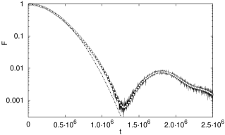
Figure 2: Long-time Gaussian decay for CIS of a single kicked top for the same parameters as in fig. 1a. Full curve is a direct numerical evaluation, empty circles are numerical calculation using the renormalized strength $\delta_{R}$ and operator $R$, while the chain curve gives the theoretical decay (14).

Long-time Gaussian decay for the parameters of fig. 1a is shown in fig. 2. Here we compare a direct numerical calculation with the numerical calculation using a renormalized perturbation strength $\delta_{R}$ and the effective perturbation operator (7) $R=\frac{-1}{2J^{3}}(J_{\rm x}J_{\rm y}J_{\rm z}+J_{\rm z}J_{\rm y}J_{\rm x})$, and with the theoretical prediction (14) where the classical dynamics of $R_{\rm cl}=-xyz$ gives $\sigma=5.1\cdot 10^{-3}$.

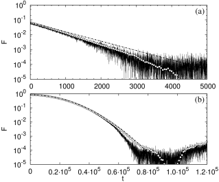
Figure 3: Long-time fidelity decay in two coupled kicked tops. For strong perturbation $\delta=7.5\cdot 10^{-2}$ (a) we obtain an exponential decay, and for smaller $\delta=2\cdot 10^{-2}$ (b) we have a Gaussian decay. Meaning of the curves is the same as in fig. 2.

To demonstrate the possibility of clean exponential long-time decay of fidelity (13) we look at a system of two ($d=2$) coupled tops $\vec{J}_{1}$ and $\vec{J}_{2}$ given by a propagator $U=\exp{(-{\rm i}\varepsilon J_{\rm z1}J_{\rm z2})}\exp{(-{\rm i}\pi J_{\rm y1}/2)}\exp{(-{\rm i}\pi J_{\rm y2}/2)},$ with the perturbation generated by $W=A_{1}\otimes\mathbbm{1}+\mathbbm{1}\otimes A_{2}$, where $A=J_{\rm z}^{2}/2J^{2}$ for each top. We set $J=1/\hbar=100$, and $\varepsilon=20$ in order to be in a fully chaotic regime. The initial state is always a direct product of SU(2) coherent states centered at $(\varphi,\theta)=(1,1)$ which is subsequently projected on an invariant subspace of dimension ${\cal N}=J(J+1)$ spanned by $\{{\cal H}_{\rm OE}\otimes{\cal H}_{\rm r}\}_{\rm sym}$, where ${\cal H}_{\rm r}={\cal H}\setminus{\cal H}_{\rm OE}$ and $\{\cdot\}_{\rm sym}$ is a subspace symmetric with respect to the exchange of the two tops. The results of numerical simulation are shown in fig. 3. Here we show only a long-time decay, as the situation in the plateau is qualitatively the same as for $d=1$. For large enough perturbation one obtains an exponential decay shown in fig. 3 (a), while for smaller perturbation we have a Gaussian decay shown in fig. 3 (b). Numerical data have been successfully compared with the theory (13,14) using classically calculated $\sigma=9.2\cdot 10^{-3}$, and with the “renormalized” numerics using the operator $R$ (7).

In this Letter we discussed a freeze of fidelity for arbitrary quantum evolution provided only that the diagonal part of the perturbation in the basis of the unperturbed evolution exactly vanishes. The value of the plateau can be arbitrary close to $1$ and can span over arbitrary long time-ranges for sufficiently small strength of perturbation. We worked out in detail the case of systems with fully chaotic classical limit. Our result is predicted to have immediate application to quantum information processing. If combined with the inequality between the purity $I(t)$ of a reduced density matrix of a bipartite quantum system and the fidelity, namely $I(t)>|F(t)|^{2}$ PSZ , we predict that decoherence as characterized by $I(t)$ should also exhibit freeze for the particular class of perturbations. Useful discussions with T.H.Seligman and financial support by the Ministry of Education, Science and Sports of Slovenia and DAAD19-02-1-0086, ARO United States are gratefully acknowledged.

References

(1)
A. Peres, Phys. Rev. A 30, 1610 (1984);
Ph. Jacquod et al. Phys. Rev. E 64,
055203 (2001); N. R. Cerruti and S. Tomsovic, Phys. Rev. Lett. 88, 054103 (2002);
F. M. Cucchietti et al. Phys. Rev. E 65 046209 (2002);
G. Benenti and G. Casati, Phys. Rev. E 65 066205 (2002).
(2)
R. A. Jalabert and H. M. Pastawski, Phys. Rev. Lett. 86, 2490 (2001).
(3)
M. A. Nielsen and I. L. Chuang, Quantum computation and quantum information
(Cambridge Univ. Press 2000).
(4) G. Veble and T. Prosen, Phys. Rev. Lett. at press (2004).
(5) T. Prosen and M. Žnidarič, J. Phys. A 35, 1455 (2002);
see also
T. Prosen and M. Žnidarič, J. Phys. A 34, L681 (2001);
T. Prosen, Phys. Rev. E 65, 036208 (2002).
(6) T. Prosen and M. Žnidarič, New J. Phys. 5, 109 (2003).
(7) We note that the approximation (5) is accurate
for arbitrary long times, provided is sufficiently small, since
one can show directly that the third order () is again at most
proportional to .
(8) In the following, means equal in the leading order in .
(9) T. Prosen, T. H. Seligman and M. Žnidarič, Phys. Rev. A 67,
062108 (2003).