Fast simulation of a quantum phase transition in an ion-trap realisable unitary map

Abstract

We demonstrate a method of exploring the quantum critical point of the Ising universality class using unitary maps that have recently been demonstrated in ion trap quantum gates. We reverse the idea with which Feynman conceived quantum computing, and ask whether a realisable simulation corresponds to a physical system. We proceed to show that a specific simulation (a unitary map) is physically equivalent to a Hamiltonian that belongs to the same universality class as the transverse Ising Hamiltonian. We present experimental signatures, and numerical simulation for these in the six-qubit case.

I Introduction

Feynman suggested that it is possible to simulate one quantum system with anotherFeynman (1983). However, we will turn this thesis around by posing the question of what sort of a system some unitary map on a quantum computer might correspond to.

In particular, we examine the ion-trap model of quantum computing, and find that the unitary maps which have been realised on these correspond to the time evolution of Hamiltonians which are linked closely to the Ising model. Finally, we consider the considerable theoretical body of work concerned with quantum phase transitions and renormalization group theory. This will later be the key to the problem of identifying a quantum phase transition in a unitary map.

I.1 Simulating Quantum Systems

Feynman’s first conception of quantum computingFeynman (1983) held the simulation of quantum systems as a key goal. Entanglement has been described as the quintessential feature of quantum mechanicsSchrödinger (1935). In general, the arbitrary time evolution of a system is considered an NP-hardCarey and Johnson (1979) problem, as memory and processing resources increase exponentially in the size of the problem, $n$, on a classical computer. It is only for extraordinarily simple systems, or ones for which there are strong symmetries, that such calculations are tractable.

Feynman suggested that the problem could be reduced to one in polynomial time on a computer based on quantum principles. These include the ability of a quantum system to perform unitary operations on a set of quantum bits (qubits), and to exist in entangled states. Feynman showed that, in principle, it was possible to perform, in polynomial time, algorithms which were only possible in non-polynomial time on a classical computer.

Since the original formulation of the problem, the application of quantum computing to classical problems has become more common. Several algorithms have been suggested, including the Deutch-Jozsa algorithmDeutch and Jozsa (1992), Shor’s factorization algorithmShor (1994), and Grover’s searching algorithmGrover (1997). However, all of these systems are widely considered far removed from current experimental abilities.

Recently, LloydLloyd (1996) revisited Feynman’s original problem, and showed that it was possible to implement the time evolution of an arbitrary spin Hamiltonian to a particular precision, $\varepsilon$, in polynomial time. The procedure essentially involves the decomposition of a Hamiltonian into realizable (local) unitary operations, and the time-wise stepping through a Hamiltonian to some arbitrary accuracy.

It will be our desire to avoid such an abstracted simulation of a quantum system, and rather consider the possibility of finding a quantum phase transition in a quantum algorithm naturally realizable with current quantum computing experimental hardware. In this way, we will essentially reverse the Feynman thesis, and conclude that quantum algorithms (or unitary maps) will correspond to the observables of some physical system.

I.2 Ion Trap Quantum Computers and the Ising Model

DiVincenzoDiVincenzo (1995) and Barenco et al.Barenco et al. (1995) has shown that single-site rotations and two-site controlled NOTs are universal for quantum computation. Further, the Sorensen-MolmerSorensen and Molmer (1999), phase gateLiebfried et al. (2003), and indeed almost any two-site entangling gateDodd et al. (2002) are universal. Hence, they will be able to affect any unitary transformation.

Cirac and Zoller’s paperCirac and P.Zoller (1995) on cold ion-trap quantum computers introduces the use of a spatially confined ion spin as a qubit, and the excitation of vibrational modes as a means of coupling qubits. Further, it has been shown that high fidelity state-preparationRoos et al. (1999) and readoutBlatt and Zoller (1988) are feasible.

Milburn has suggested a robust phase space scheme to use ion traps to simulate nonlinear interactions in spin systemsMilburn (1999). A significant advantage of this scheme is that it does not require the cooling of vibrational states. The method involves the application of Raman pulses faster than the vibrational heating time, effectively decoupling the effect of vibrational modes. In particular, Milburn shows that the evolution of a Hamiltonian of the form

$$H_{int}=\hbar\chi\sigma_{z}^{(1)}\sigma_{z}^{(2)}$$ (1)

may be achieved by a pulse sequence

$$U_{int}=e^{-iH_{int}} = e^{i\kappa_{x}\hat{X}\sigma_{z}^{(1)}}e^{i\kappa_{p}\hat{P}\sigma_{z}^{(2)}}$$

$$e^{-i\kappa_{x}\hat{X}\sigma_{z}^{(1)}}e^{-i\kappa_{p}\hat{P}\sigma_{z}^{(2)}}$$

where $\hat{X}=\frac{a+a^{\dagger}}{\sqrt{2}}$ and $\hat{P}=\frac{a-a^{\dagger}}{i\sqrt{2}}$, and expressions for $\kappa_{x}$ and $\kappa_{p}$ given in Ref. Milburn et al. (2000).

Further, Wineland’s research group have recently demonstratedLiebfried et al. (2003) considerable success in achieving few-qubit interactions with this scheme. In particular, they present a two qubit phase gate, which has the form

$$\left|\downarrow\downarrow\right\rangle\rightarrow\left|\downarrow\downarrow\right\rangle \left|\uparrow\uparrow\right\rangle\rightarrow\left|\uparrow\uparrow\right\rangle,$$ ,

$$\left|\downarrow\uparrow\right\rangle\rightarrow e^{i\phi}\left|\downarrow\uparrow\right\rangle \left|\uparrow\downarrow\right\rangle\rightarrow e^{i\phi}\left|\uparrow\downarrow\right\rangle$$ .

which can be recast as $\left|\Psi\right\rangle\rightarrow e^{-i\chi\sigma_{x}^{(1)}\sigma_{x}^{(2)}}\left|\Psi\right\rangle$. Apart from an uninteresting global additive phase, this may be considered to model the time evolution of a Hamiltonian of the form $\sigma_{x}^{(n)}\sigma_{x}^{(n+1)}$.

Further, it is well known that single rotations in any basis, which correspond to the evolution of a spin operator, are easily implementable on such an architectureCirac and P.Zoller (1995). They result in unitary transformations of the form

$$U_{single}=e^{-i\hbar\theta\sigma_{x}^{(1)}}$$ (3)

which can be implemented trivially through a single Raman pulse.

Following Feynman’s original intentions for quantum computing, one may consider the mapping of Hamiltonian with such terms onto an ion-trap quantum computer. Turning this problem around, we will consider the properties of a unitary map composed of terms which can be experimentally implemented, and investigate their relationship with the transverse Ising spin chain.

I.3 Quantum Phase Transitions and Universality Classes

The quantum phase transition in the one dimensional transverse Ising modelSachdev (2000) is very well understood. The Hamiltonian is given by:

$$H_{Ising}=\sum_{n=1}^{N}\mu B\sigma_{x}^{(n)}+J\sigma_{z}^{(n)}\sigma_{z}^{(n)}$$ (4)

It is known that for an external field with interaction strength $\mu B$ and local exchange interaction term with strength $J$, that a phase transition occurs for $\mu B=\pm J$. One can intuitively consider the phase transition as a result of the incongruent symmetries between the two phases, which is reflected in the difference in behaviour of the two terms in the Hamiltonian under the transformation $\sigma_{n}\rightarrow-\sigma_{n}$. In the regime $J>\mu B$, the system is in a ferromagnetic phase, with $\left\langle\sigma_{x}^{(n)}\right\rangle\neq 0$, and the system displays long range order. On the other hand, for $J<\mu B$, the system is paramagnetic, with$\left\langle\sigma_{x}^{(n)}\right\rangle=0$, and there is no broken symmetry.

Using arguments from renormalization group theory, we may place a great number of related problems into the same universality classCardy (1996), and we may expect to see a similar phase transition occur in a number of related systems.

II The Model

In the following, we will put together the components introduced in Section I in a intuitive way. We consider the composition of the two unitary maps, similar to those demonstrated in Ref Liebfried et al. (2003), which corresponds to the composition of the time evolution of two Hamiltonians. In form, it will look similar to the one-dimensional transverse Ising chain Hamiltonian. We will then apply the Jordan-Wigner transformation to this model to express the Hamiltonians in terms of non-interacting fermions. We are then able to perform a composition of operators in an $SU(2)$ representation to yield a single Hamiltonian. We will find that this model is highly non-local. However, using renormalization group theory concepts, it can be shown that the Hamiltonian belongs in the same universality class as the transverse Ising chain. Hence, we conclude that our separated model has the same quantum phase transition as the transverse Ising chain, even though we have implemented the map in a much simpler way.

II.1 Model Unitary Transformation and Experimental Realization

It is natural to decompose the Ising Hamiltonian, $H_{Ising}$ into two distinct parts:

$$H_{\chi}=\chi\sum_{n=1}^{N}\sigma_{z}^{(n)}\sigma_{z}^{(n+1)}$$ (5)

$$H_{\theta}=\theta\sum_{n=1}^{N}\sigma_{x}^{(n)}$$ (6)

These parts are of even and odd symmetry under $\vec{\sigma_{n}}\rightarrow-\vec{\sigma_{n}}$, respectively. Unitary maps of the form $\left|\Psi\right\rangle\rightarrow e^{iH_{\chi,\theta}}\left|\Psi\right\rangle$ have been realised experimentally. It is impossible to perform them both at the same time with only single qubit rotations and two qubit gates, because they do not commute - the evolution of the combined Hamiltonian is not the composition of the evolutions of both Hamiltonians. Note however that terms $\sigma_{z}^{(n)}\sigma_{z}^{(n+1)}$ and $\sigma_{z}^{(m)}\sigma_{z}^{(m+1)}$ do commute, and so

$$e^{iH_{\chi}}=\prod_{n=1}^{N}e^{i\chi\sigma_{z}^{(n)}\sigma_{z}^{(n+1)}}$$ (7)

is realisable in principle with current technology.

The combined Hamiltonian may be approximated by Lloyd’sLloyd (1996) methods, which involves applying terms such as $\frac{1}{m}H_{\chi}$ and $\frac{1}{m}H_{\theta}$ repeatedly, $m$ times. However this requires a large overhead - instead we will consider the unitary map

$$U(\chi,\theta)=e^{-iH_{\chi}}e^{-iH_{\theta}}=e^{-i\bar{H}}\neq e^{-i(H_{\chi}+H_{\theta})}$$ (8)

This map has been proposed by Milburn et al. Milburn et al. (2000) as an easier unitary map to to simulate than the map which corresponds to the time evolution of transverse Ising chain Hamiltonian. We are interested in whether this mapping will have the same quantum phase transition behaviour as the transverse Ising chain.

II.2 Jordan-Wigner Transformation

We will follow Jordan and WignerJordan and Wigner (1928) in using the following definitions to introduce a new set of operators, $a_{n}$, where

$$\sigma_{x}^{(n)} = 1-2a_{n}a_{n}^{\dagger}$$ (9)

$$\sigma_{y}^{(n)} = -i(a_{n}-a_{n}^{\dagger})$$ (10)

$$\sigma_{z}^{(n)} = a_{n}^{\dagger}+a_{n}$$ (11)

where $\sigma_{x}^{(n)}$, $\sigma_{y}^{(n)}$ and $\sigma_{z}^{(n)}$ take the form of the Pauli spin matrices in the $\left|0\right\rangle$,$a_{n}^{\dagger}\left|0\right\rangle$ basis. From these definitions, the operators $a_{n}$ and $a_{n}^{\dagger}$ can be shown to obey the following relations:

$$\{a_{n}^{\dagger},a_{n}\}=1, a_{n}^{2}=0, a_{n}^{\dagger^{2}}=0,$$

$${}[a_{m}^{\dagger},a_{n}]=0, [a_{m}^{\dagger},a_{n}^{\dagger}]=0, [a_{m},a_{n}]=0,m\neq n$$

With these definitions, our unitary map becomes

$$U(\chi,\theta) = e^{-i\chi\sum_{n=1}^{N}a_{n}^{\dagger}a_{n+1}^{\dagger}+a_{n}a_{n+1}+a_{n}a_{n+1}^{\dagger}+a_{n}^{\dagger}a_{n+1}}$$

$$e^{-i\theta\sum_{n=1}^{N}1-2a_{n}a_{n}^{\dagger}}$$

We then introduce the following operators

$$c_{n} = e^{i\pi\sum_{j=1}^{n-1}a_{j}^{\dagger}a_{j}}a_{n}$$ (13)

$$c_{n}^{\dagger} = a_{n}^{\dagger}e^{-i\pi\sum_{j=1}^{n-1}a_{j}^{\dagger}a_{j}}$$ (14)

It can be shown that they obey fermionic anti-commutation relations.

We may understand these as an expression of domain wall creation and destruction. We can re-express $U(\chi,\theta)$ with this new set of operators as

$$U(\chi,\theta) = e^{-i\chi\sum_{n=1}^{N}c_{n}^{\dagger}c_{n+1}^{\dagger}-c_{n}c_{n+1}-c_{n}c_{n+1}^{\dagger}+c_{n}^{\dagger}c_{n+1}}$$

$$e^{-i\theta\sum_{n=1}^{N}c_{n}^{\dagger}c_{n}-c_{n}c_{n}^{\dagger}}$$

Finally, we will define the Fourier transformed versions of the fermion operators as

$$c_{n} = \frac{1}{\sqrt{N}}\sum_{k}C_{k}e^{ink}$$ (16)

$$c_{n}^{\dagger} = \frac{1}{\sqrt{N}}\sum_{k}C_{k}^{\dagger}e^{-ink}$$ (17)

However, it is important to take note of the boundary terms. Strictly, in order to have Eqs. (8) and (II.2) identical, we must make the identificationLieb et al. (1961)

$$c_{N+1}=c_{1}(e^{i\sum_{j=1}^{N}c_{j}^{\dagger}c_{j}}+1)$$

It may be argued that in the thermodynamic limit, this term will be irrelevant, and we may make the identification $c_{N+1}=c_{1}$.

Due to cyclic boundary conditions, we will require $k$ to take the discrete values

$$k=\frac{2\pi m}{L},m=-\frac{L}{2},...,-1,0,1,\frac{L-2}{2}$$

These operators satisfy fermion anti-commutation relations:

$$\{C_{k},C_{l}^{\dagger}\} = \delta_{kl}$$

$$\{C_{k},C_{l}\} = \{C_{k}^{\dagger},C_{l}^{\dagger}\}=0$$

Using the definitions of $c_{n}$ and $c_{n}^{\dagger}$, and the thermodynamic limit we can re-write $U(\chi,\theta)$ as

$$U(\chi,\theta) = e^{-i\chi\sum_{k}2\cos kC_{k}^{\dagger}C_{k}-i\sin k(C_{k}^{\dagger}C_{-k}^{\dagger}+C_{k}C_{-k})}$$

$$e^{-i\theta\sum_{k}(2C_{k}^{\dagger}C_{k}-1)}$$

where we require the thermodynamic limit so that the property $2\sum_{k}C_{k}^{\dagger}C_{k}=\sum_{k}(C_{k}^{\dagger}C_{k}+C_{-k}^{\dagger}C_{-k})$ holds.

To simplify matters, let us further define

$$\hat{A}_{k} = \chi(2\cos kC_{k}^{\dagger}C_{k}-i\sin k(C_{k}^{\dagger}C_{-k}^{\dagger}+C_{k}C_{-k}))$$ (19)

$$\hat{B}_{k} = \theta(2C_{k}^{\dagger}C_{k}-1)$$ (20)

such that we may write

$$U(\chi,\theta)=e^{-i\sum_{k}\hat{A}_{k}}e^{-i\sum_{k}\hat{B}_{k}}=\Pi_{k}U_{k}(\chi,\theta)$$ (21)

where $U_{k}(\chi,\theta)\equiv e^{-i\hat{A}_{k}}e^{-i\hat{B}_{k}}$.

We have now completely decoupled the problem, and may express the operators $\hat{A_{k}}$ and $\hat{B_{k}}$ in the basis $\left|0\right\rangle,C_{k}^{\dagger}\left|0\right\rangle,C_{-k}^{\dagger}\left|0\right\rangle,C_{k}^{\dagger}C_{-k}^{\dagger}\left|0\right\rangle$. It is be possible to find eigenstates of $U(\chi,\theta)$ in closed form in this basis.

II.3 Combining

However, it would be nice to be able to express $U(\chi,\theta)$ as a single exponential. While $\hat{A_{k}}$ and $\hat{B_{k}}$ do not commute, it turns out that there is a faithful representation in $SU(2)$, if we make the following definitions :

$$\nu_{1}^{(k)} = -i(C_{k}^{\dagger}C_{-k}^{\dagger}+C_{k}C_{-k})$$

$$\nu_{2}^{(k)} = (-C_{k}^{\dagger}C_{-k}^{\dagger}+C_{k}C_{-k})$$

$$\nu_{3}^{(k)} = C_{k}^{\dagger}C_{k}+C_{-k}^{\dagger}C_{-k}-I$$

Hence, we can express $\hat{A}_{k}=\chi(\cos k+\vec{\alpha}.\vec{\nu_{k}})$ and $\hat{B}_{k}=\theta\vec{\beta}_{k}.\vec{\nu}_{k}$, where $\vec{\alpha}_{k}=\chi(\sin k,0,\cos k)$ and $\vec{\beta}_{k}=\theta(0,0,1)$. We have that $[\nu_{l}^{(k)},\nu_{m}^{(k^{\prime})}]=-2i\epsilon_{l,m,n}\nu_{n}^{(k)}\delta_{k}^{k^{\prime}}$ where $\epsilon_{l,m,n}$ is the Levi-Civita symbol, so that $\{\nu_{1}^{(k)},\nu_{2}^{(k)},\nu_{3}^{(k)}\}$ have the same properties as the $SU(2)$ matrices $\{\sigma_{1},\sigma_{2},\sigma_{3}\}$. Relating the fermionic operators to $SU(2)$ in this way was inspired by a similar approach in the theory of superconductorsSchrieffer (1964).

$SU(2)$ is closed under composition with a well understood composition relation, which we can now apply to our systemVaradarajan (1984)

$$U_{k}(\chi,\theta)=e^{-i\chi\vec{\alpha}_{k}.\vec{\nu_{k}}}e^{-i\theta\vec{\beta}_{k}.\vec{\nu_{k}}}=e^{-i\cos k}e^{-i\kappa_{k}\vec{\gamma}_{k}(\chi,\theta).\vec{\nu_{k}}}$$ (22)

where

$$\vec{\gamma}_{k}(\chi,\theta) = (\sin k\cos\theta\sin\chi,-\sin k\sin\theta\sin\chi,$$

$$(\sin\theta\cos\chi+\cos k\cos\theta\sin\chi))$$

$$\kappa_{k} = {\frac{\cos^{-1}\eta_{k}}{\sqrt{1-\eta_{k}^{2}}}}$$ (24)

$$\eta_{k} = \cos\theta\cos\chi-\cos k\sin\theta\sin\chi$$

$$= \cos^{2}\frac{k}{2}\cos(\theta+\chi)+\sin^{2}\frac{k}{2}\cos(\theta-\chi)$$

This composition has the simple physical interpretation of two rotations being composed, and the result can be derived using quaternion compositionHerstein (1964). However, when using quaternions, special care has to be given to the double cover of $SO(3)$ under $SU(2)$. The second equality of Eq. (22) defines an effective Hamiltonian, $\bar{H}_{k}$, and we stress that $\bar{H}_{k}\neq\hat{A}_{k}+\hat{B}_{k}$ because $\hat{A}_{k}$and $\hat{B}_{k}$ do not commute.

Hence, we have the final form of the decoupled, and combined transformation

$$U(\chi,\theta)=\Pi_{k}U_{k}(\chi,\theta)=e^{-i\sum_{k}\kappa_{k}\vec{\gamma}_{k}(\chi,\theta).\vec{\nu_{k}}}$$ (26)

Hence, we have found that the effective Hamiltonian , $\bar{H}$, defined in Eq (8) is given by $\bar{H}=\sum_{k}\kappa_{k}\vec{\gamma}_{k}(\chi,\theta).\vec{\nu_{k}}$

We now check the limit $\chi\rightarrow 0$, which implies $\kappa\rightarrow{\frac{\theta}{\sin\theta}}$, and $\vec{\gamma}_{k}\rightarrow\{0,0,\cos k\sin\theta\}$. Hence $U(\chi,\theta)=e^{-i\sum_{k}{\frac{\theta}{\sin\theta}}\sin\theta\cos k\nu_{3}}=e^{-i\theta\sum_{k}{\frac{-i}{2}}\sigma_{x}\sigma_{y}-\sigma_{y}\sigma_{x}}=e^{-i\theta\sum_{k}{\frac{-i}{2}}2i\sigma_{x}\sigma_{y}}=e^{-i\theta\sum_{k}\sigma_{z}}$. On the other hand, in the limit $\theta\rightarrow 0$, $\kappa={\frac{\chi}{\sin\chi}}$, and $\vec{\gamma}_{k}=\{\sin\chi\sin k,0,\sin\chi\cos k\}$. Hence $U(\chi,\theta)=e^{-i\chi\sum_{k}\sin k\nu_{1}+\cos_{k}\nu_{3}}$. Thus, we retrieve the expected behaviour in the limit as we turn off either the exchange or external field terms.

Having expressed $U(\chi,\theta)$ in this form, it is now possible to show that it directly corresponds to some physical Hamiltonian. We may perform a Bogoliubov transformation by defining some fermion creation operator

$$\gamma_{k}\gamma_{k}^{\dagger}=\vec{\gamma}_{k}(\chi,\theta).\vec{\nu_{k}}$$ (27)

with associated energy, $\epsilon_{k}=\kappa_{k}$. Hence, we may consider our ground state as a vacuum state $|0>$, and excitations as $\gamma_{k}^{\dagger}\left|0\right\rangle$. It is important to note here that the excitations of lowest energy will occur at an extremum of $\epsilon_{k}$. We can show that this occurs at $k=0,\pi$ by noting that

$$\frac{\partial\epsilon_{k}}{\partial k}=\frac{\partial\kappa_{k}}{\partial k}=\frac{\partial\kappa_{k}}{\partial\eta_{k}}\frac{\partial\eta_{k}}{\partial k}$$ (28)

from which it follows that

$$\left.\frac{\partial\eta_{k}}{\partial k}\right|_{k=0,\pi}=\left.\sin k\sin\theta\sin\chi\right|_{k=0,\pi}=0$$ (29)

Hence, the elementary excitations will be for $k=0$ or $k=\pi$, whichever corresponds to a lower energy.

II.4 Closed-form Hamiltonian

We can now work backwards from our expression for $U(\chi,\theta)$ to a single combined Hamiltonian. The results here will only be valid in the thermodynamic limit, which we have assumed in the previous section. Before doing so, we should present a list of identities which will prove to be useful.

$$\sum_{k}e^{iak}\nu_{1}^{(k)} = i\sum_{n}c_{n}^{\dagger}c_{n+a}^{\dagger}-c_{n}c_{n+a}$$

$$\sum_{k}e^{iak}\nu_{2}^{(k)} = -\sum_{n}c_{n}^{\dagger}c_{n+a}^{\dagger}+c_{n}c_{n+a}$$

$$\sum_{k}e^{iak}\nu_{3}^{(k)} = \sum_{n}2c_{n}^{\dagger}c_{n}-I$$

$$\sum_{k}\nu_{1}^{(k)}=0 \sum_{k}\cos(ak)\nu_{1}^{(k)}=0$$ ,

$$\sum_{k}\sin(ak)\nu_{1}^{(k)} = \sum_{n}c_{n}^{\dagger}c_{n+a}^{\dagger}-c_{n}c_{n+a}$$

$$\sum_{k}\nu_{2}^{(k)}=0 \sum_{k}\cos(ak)\nu_{2}^{(k)}=0$$ ,

$$\sum_{k}\sin(ak)\nu_{2}^{(k)} = i\sum_{n}(c_{n}^{\dagger}c_{n+a}^{\dagger}+c_{n}c_{n+a})$$

Now, recall that

$$U(\chi,\theta)=e^{-i\sum_{k}\kappa_{k}\vec{\gamma}_{k}(\chi,\theta).\vec{\nu}_{k}}$$ (30)

However, $\kappa_{k}$ is an even function of $k$, and so can be expanded in terms of a Fourier series involving $\cos k$. Let us write

$$\kappa_{k}=\sum_{l=0}^{\infty}a_{l}\cos(lk)$$ (31)

$$U(\chi,\theta)=e^{-i\sum_{k,l}a_{l}\cos(lk)\vec{\gamma}_{k}(\chi,\theta).\vec{\nu}_{k}}$$ (32)

We will now substitute our expression for $\vec{\gamma}_{k}$ and expand.

$$U(\chi,\theta) = e^{-i\sum_{k,l}a_{l}\cos lk\vec{\gamma_{k}}(\chi,\theta).\vec{\nu}_{k}}$$ (33)

$$= e^{-i(\Lambda_{1}+\Lambda_{2}+\Lambda_{3})}$$ (34)

$$= e^{-i\bar{H}}$$ (35)

where

$$\Lambda_{1} = \cos\theta\sin\chi\sum_{k,l}a_{l}\sin k\cos(lk)\nu_{1}^{(k)}$$ (36)

$$\Lambda_{2} = -\sin\theta\sin\chi\sum_{k,l}a_{l}\sin k\cos(lk)\nu_{2}^{(k)}$$ (37)

$$\Lambda_{3} = \sin\theta\cos\chi\sum_{k,l}a_{l}\cos(lk)\nu_{3}^{(k)}$$

$$+\cos\theta\sin\chi\sum_{k,l}a_{l}\cos k\cos(lk)\nu_{3}^{(k)}$$

and the sum over $l$ ranges $1,2,3...$

We may rewrite this as

$$\Lambda_{1} = \cos\theta\sin\chi\sum_{k,l}a_{l}[\sin(l+1)k-\sin(l-1)k]\nu_{1}^{(k)}$$ (39)

$$= \cos\theta\sin\chi[a_{0}(c_{n}^{\dagger}c_{n+1}^{\dagger}-c_{n}c_{n+1})$$

$$+\sum_{n,l}\frac{(a_{l+1}-a_{l-1})}{2}(c_{n}^{\dagger}c_{n+l}^{\dagger}-c_{n}c_{n+l})]$$

$$\Lambda_{2} = -\sin\theta\sin\chi\sum_{k,l}a_{l}[\sin(l+1)k-\sin(l-1)k]\nu_{2}^{(k)}$$ (41)

$$= -i\sin\theta\sin\chi\sum_{n,l}[a_{o}(c_{n}^{\dagger}c_{n+1}^{\dagger}+c_{n}c_{n+1})$$

$$+\sum_{l}\frac{(a_{l+1}-a_{l-1})}{2}(c_{n}^{\dagger}c_{n+l}^{\dagger}+c_{n}c_{n+l})]$$

$$\Lambda_{3} = \sin\theta\cos\chi\sum_{k,l}a_{l}\cos(lk)\nu_{3}^{(k)}$$

$$+\cos\theta\sin\chi\sum_{k,l}a_{l}[\cos(l+1)k+\cos(l-1)k]\nu_{3}^{(k)}$$

$$= \sin\theta\cos\chi\sum_{l}[a_{l}(c_{n}^{\dagger}c_{n+l}-c_{n}c_{n+l}^{\dagger})]+$$

$$+\cos\theta\sin\chi\sum_{n,l}[a_{0}(c_{n}^{\dagger}c_{n+1}-c_{n}c_{n+1}^{\dagger})$$

$$+\frac{(a_{l+1}-a_{l-1}))}{2}(c_{n}^{\dagger}c_{n+l}-c_{n}c_{n+l}^{\dagger})]$$

Therefore, the quantum spin chain Hamiltonian $\bar{H}$ which represents a physical system corresponding to the separated unitary map (8) is highly non-local. Terms such as $c_{n}c_{n+a}^{\dagger}=a_{n}e^{-i\pi\sum_{j=n}^{n+a-1}a_{j}a_{j}^{\dagger}}a_{n+a}^{\dagger}$ for $a>1$ will not only involve $a_{n},a_{n+a}$, but also $c_{m}$ and $c_{m}^{\dagger}$ $\forall n<m<n+a$.

If we define

$$\sigma_{+}^{(n)} = \frac{\sigma_{z}^{(n)}+i\sigma_{y}^{(n)}}{2}$$

$$\sigma_{-}^{(n)} = \frac{\sigma_{z}^{(n)}-i\sigma_{y}^{(n)}}{2}$$

we can write $c_{n}c_{n+a}^{\dagger}$ as $\sigma_{+}^{(n)}e^{-i\pi\sum_{j=n}^{n+a-1}\frac{1-\sigma_{x}^{(j)}}{2}}\sigma_{-}^{(n+a)}$, explicitly showing the dependence on non-neighbouring spins.

II.5 Range of the Interactions

To be in the universality class of the Ising model, we would expect the non-local terms, $a_{l}$ to decrease exponentially with separation $l$. Thus, when viewed at larger length scales, the non-local terms would become irrelevant. The behaviour of $a_{n}$ for a variety of $\theta=\chi$ is calculated numerically and presented in Fig. 1. The case for $\theta\neq\chi$ is similar, and displays the same exponential decrease in $a_{l}$ with $l$. Hence, we may naturally expect nearest-neighbour interactions to be the most important interactions in this model - an idea which we will make concrete in the following section.

Figure 1: The behaviour of Fourier coefficients $a_{n}$, as defined in Eq. 32, for $n=1,2...10$ for a variety of $\theta$ and $\chi$. Note that the larger $\left|\chi-\frac{\pi}{2}\right|$ and $\left|\theta-\frac{\pi}{2}\right|$, the larger the decay. The exponential decay in these coefficients implies that the interactions in the Hamiltonian are short-ranged, and suggests that renormalization techniques should be highly effective in this model.

Deriving an analytic expression for $a_{n}$ seems to be very difficult. However it is possible to show a general dependence on $\theta$ and $\chi$ of the form $\sin^{n}\theta\sin^{n}\chi$ for any particular $n$. We can expand $\kappa_{k}$ in terms of $\eta_{k}$, where $\eta_{k}$ is defined in Eq. (II.3), as

$$\kappa_{k}=\sum_{p=0}^{\infty}\frac{2^{p-q}\Gamma^{2}(\frac{p+1}{2})}{\Gamma(p+1)}\eta_{k}^{p}=\sum_{p=0}^{\infty}c_{p}\eta_{k}^{p}$$ (45)

where $\Gamma$ is the Euler gamma function. In turn, $\eta^{p}$ can be expressed as a series in terms of $\cos^{q}k$ as

$$\eta_{k}^{p} = \sum_{q=0}^{p}\left(\begin{array}[]{c}p\\ q\end{array}\right)(\cos\theta\cos\chi)^{p-q}(-\cos k\sin\theta\sin\chi)^{q}$$

$$= \sum_{q=0}^{p}d_{p,q}\cos^{q}k$$

Finally, we can express $\cos^{q}k$ in terms of $\cos rk$. For the case of $q$ even, this is

$$\cos^{q}k = \sum_{r=0,r\in evens}^{q}\left(\begin{array}[]{c}q\\ \frac{q-r}{2}\end{array}\right)\frac{\cos rk}{2^{q-1}}+c$$

$$= \sum_{r=0}^{q}e_{q,r}\cos rk$$

where $c$ is an unenlightening constant, and a similar expression holds for $p-q$ odd.

We can combine Equations (45),(II.5) and (II.5) to yield an expression for $\kappa_{k}$

$$\kappa_{k}=\sum_{p=0}^{\infty}c_{p}\eta^{p}=\sum_{p=0}^{\infty}\sum_{q=0}^{p}\sum_{r=0}^{q}c_{p}d_{p,q}e_{q,r}\cos rk$$ (52)

from which we can read the coefficient $a_{l}$ of $\cos lk$ as

$$a_{l}=\sum_{p=0}^{\infty}c_{p}\eta^{p}=\sum_{p=0}^{\infty}\sum_{q=0}^{p}c_{p}d_{p,q}e_{q,l}$$ (53)

However, $e_{q,l}$ is only non-zero for $q>l$, and so we can replace $\sum_{q=0}^{p}$ with $\sum_{q=l}^{p}$ to yield

$$a_{l} = \sum_{p=0}^{\infty}c_{p}\eta^{p}=\sum_{p=0}^{\infty}c_{p}\sum_{q=l}^{p}d_{p,q}e_{q,l}$$ (54)

which involves terms in $d_{p,q}\propto(\sin\theta\sin\chi)^{q}(\cos\theta\cos\chi)^{s}$ for $q>l$. Hence, for any given $a_{l}$, there is a behaviour proportional to $(\sin\theta\sin\chi)^{l}$.

Of physical interest is the behaviour of $a_{l}$ with respect to $l$ for a given $\theta$ and $\chi$. We will attempt to factor out any behaviour in $l$ by noting that since $d_{pq},e_{q,l}<1$, we can write

$$a_{l} = \sum_{p=0}^{\infty}c_{p}\sum_{q=l}^{p}d_{p,q}e_{q,l}$$

$$\leq \sum_{p=0}^{\infty}c_{p}\sum_{q=l}^{p}d_{p,q}\sum_{q=l}^{p}e_{q,l}$$

However, if we turn our attention to the sum over $d_{p,q}$, we can construct a further limit on $a_{l}$

$$\sum_{q=l}^{p}d_{p,q} = \sum_{q=l}^{p}\left(\begin{array}[]{c}p\\ q\end{array}\right)(\cos\theta\cos\chi)^{p-q}(-\cos k\sin\theta\sin\chi)^{q}$$ (58)

$$\leq \sum_{q^{\prime}=0}^{p-l}\left(\begin{array}[]{c}p\\ q^{\prime}+l\end{array}\right)(\cos\theta\cos\chi)^{p-q^{\prime}-l}(\sin\theta\sin\chi)^{q^{\prime}+l}$$ (61)

$$\leq \sum_{q^{\prime}=0}^{p-l}\left(\begin{array}[]{c}p-l\\ q^{\prime}\end{array}\right)(\cos\theta\cos\chi)^{p-l-q^{\prime}}(\sin\theta\sin\chi)^{q^{\prime}+l}$$ (64)

$$\leq (\sin\theta\sin\chi)^{l}(\cos\theta\cos\chi+\sin\theta\sin\chi)^{p-l}$$ (65)

$$\leq (\sin\theta\sin\chi)^{l}$$ (66)

Leading to our strictest inequality for $a_{l}$, showing an exponential decay in $l$

$$a_{l} \leq (\sin\theta\sin\chi)^{l}\sum_{p=0}^{\infty}c_{p}\sum_{q=l}^{p}e_{q,l}$$ (67)

$$\leq (\sin\theta\sin\chi)^{l}(\sum_{p=0}^{\infty}c_{p}p\max_{q}e_{q,l})$$ (68)

The case $\theta,\chi\rightarrow\frac{\pi}{2}$ has asymptotically constant $a_{l}$. However, for $\theta,\chi\neq\frac{\pi}{2}$, we can say that

$$a_{l}\leq ke^{-\mu l}\rightarrow 0 \mathrm{\mathrm{as}} l\rightarrow\infty$$ (69)

where $\mu=\ln(\sin\theta\sin\chi)$. Thus the terms in our model $\bar{H}$ has only short range interactions.

II.6 Renormalizing the Hamiltonian

We have seen that the Hamiltonian, $\bar{H}$, associated with the complete unitary $U$ is very complicated and involves non-local interactions. Hence, we are forced to use renormalization group methods to extract the interesting physics from this case.

Consider the continuum limit of the Hamiltonian, $\bar{H}$, which is applicable in the thermodynamic limit. Near criticality, the physics will be driven by long-wavelength effects, which suggest that the wavevector $k$ will be small. The relevant excitations at low temperature happen at the extremum of $\epsilon_{k}$, which we have shown occurs at $k=0$. Hence, in the continuum limit, we can consider only low lying states, near $k=0$. Under these approximations, our Hamiltonian becomes

$$\bar{H}\simeq\bar{H}^{\prime} = \sum_{k}\bar{\kappa}\vec{\bar{\gamma}}_{k}(\chi,\theta).\vec{\nu}_{k}$$ (70)

$$\vec{\bar{\gamma}}_{k} = (k\cos\theta\sin\chi,-k\sin\theta\sin\chi,\sin(\theta+\chi))$$ (71)

$$\bar{\kappa} = \frac{\theta+\chi}{\sin(\theta+\chi)}$$ (72)

which yields in terms if the fermion operators

$$\bar{H}^{\prime} = \sum_{k}ik\frac{(\theta+\chi)\sin\chi}{\sin(\theta+\chi)}(e^{i\theta}C_{k}^{\dagger}C_{-k}^{\dagger}+e^{-i\theta}C_{k}C_{-k})$$

$$+2(\theta+\chi)C_{k}^{\dagger}C_{k}$$

Defining the continuum Fermi fieldFradkin (1991) as

$$\Psi(x_{i})=\frac{1}{\sqrt{a}}c_{i}$$ (74)

where $a$ is the lattice spacing. $\Psi(x)$ satisfies the usual anti-commutation relation $\{\Psi(x),\Psi^{\dagger}(x^{\prime})\}=\delta(x-x^{\prime})$. Note that we can replace the sum over $k$ with an integral, by making the substitution

$$\sum_{k}a\rightarrow\int dx$$

Further, we expand the terms $C_{k}^{\dagger}C_{-k}^{\dagger}$ and $C_{k}C_{-k}$ into terms of first order gradients $\frac{\partial\Psi^{\dagger}}{\partial x}$ and $\frac{\partial\Psi}{\partial x}$ through the use of identities (Chapter 4 of Ref. Sachdev (2000)). This yields

$$\bar{H}^{\prime}\simeq\tilde{H} = E_{0}+\int dx[\frac{(\theta+\chi)\sin\chi}{\sin(\theta+\chi)}(e^{i\theta}\Psi^{\dagger}\frac{\partial\Psi^{\dagger}}{\partial x}-e^{-i\theta}\Psi\frac{\partial\Psi}{\partial x})$$

$$-2(\theta+\chi)\Psi^{\dagger}\Psi]$$

and $E_{0}$ is some constant.

Applying the transformation $\Psi\rightarrow e^{i\frac{\theta}{2}}\Psi$, we have that

$$\tilde{H} = E_{0}+\int dx[\frac{(\theta+\chi)\sin\chi}{\sin(\theta+\chi)}(\Psi^{\dagger}\frac{\partial\Psi^{\dagger}}{\partial x}-\Psi\frac{\partial\Psi}{\partial x})$$

$$-2(\theta+\chi)\Psi^{\dagger}\Psi]$$

If we do not perform this transformation, we will have terms of the form $\int dx\frac{\partial\Psi^{\dagger}}{\partial x}+\Psi\frac{\partial\Psi}{\partial x}$ in the Hamiltonian. One can show that these terms correspond to interactions of the form $\sigma_{z}^{(n)}\sigma_{y}^{(n+1)}+\sigma_{y}^{(n)}\sigma_{z}^{(n+1)}$. Chapter 4 of Ref. Fradkin (1991) has further details regarding these sorts of chiral symmetries in systems.

One can show that the Lagrangian corresponding to this Hamiltonian will then be

$$\mathcal{\tilde{L}} = \Psi^{\dagger}\frac{\partial\Psi}{\partial\tau}+\frac{(\theta+\chi)\sin\chi}{\sin(\theta+\chi)}(\Psi^{\dagger}\frac{\partial\Psi^{\dagger}}{\partial x}-\Psi\frac{\partial\Psi}{\partial x})$$

$$-2(\theta+\chi)\Psi^{\dagger}\Psi$$

where $\tau$ is imaginary time.

Now we introduce the crucial step where we considering the effect of scaling the problem. If we consider the effect of viewing the problem at a scale $\delta^{l}$ more coarse in space, and $\delta^{zl}$ more coarse in time, we can introduce the new variables

$$x^{\prime} = x\delta^{-l}$$ (78)

$$\tau^{\prime} = \tau\delta^{-zl}$$ (79)

$$\Psi^{\prime} = \Psi\delta^{l/2}$$ (80)

We choose the value of the dynamic critical exponent, $z$, to be identically equal to $1$, corresponding to an isotropy between space and time, in order to leave the velocity-like coefficients of $\Psi^{\dagger}\frac{\partial\Psi^{\dagger}}{\partial x}$ and $\Psi\frac{\partial\Psi}{\partial x}$ unchanged.

For criticality to hold, these scaling conditions must leave the Lagrangian unchanged. This occurs only when the quantity $\theta+\chi$ is identically zero. This happens for $\theta=-\chi$, exactly as in the transverse Ising model.

Formally, if we write

$$\tilde{\mathcal{L}}=\Psi^{\dagger}\frac{\partial\Psi}{\partial\tau}+u(\Psi^{\dagger}\frac{\partial\Psi^{\dagger}}{\partial x}-\Psi\frac{\partial\Psi}{\partial x})+\Delta\Psi^{\dagger}\Psi$$ (81)

we will require that

$$\Delta^{\prime} = \Delta\delta^{l}$$ (82)

$$u^{\prime} = u$$ (83)

implying that the scaling dimension of the term $\Delta\Psi^{\dagger}\Psi$,$\dim(\Delta)=1$. Hence, $u$, and $\Delta$ are relevant parameters, having non-negative scaling factors.

If we include second (or higher) order effects in $k$, we will include terms of the form $\Delta^{\prime}\Psi^{\dagger}\frac{\partial^{2}\Psi}{\partial x^{2}}$ or $\Delta^{\prime\prime}\Psi^{\dagger}\frac{\partial\Psi^{\dagger}}{\partial x}\frac{\partial\Psi}{\partial x}\Psi$ (or higher derivatives). From a simple analysis, one can show that the parameters $\Delta^{\prime}$ and $\Delta^{\prime\prime}$ are irrelevant, as the scaling dimensions areSachdev (2000)

$$\dim(\Delta^{\prime})=-1 \dim(\Delta^{\prime\prime})=-2$$ ,

Recall the Ising chain in a transverse field, Eq. (4), given by

$$H_{Ising} = \sum_{n=1}^{N}\mu B\sigma_{x}^{(n)}+J\sigma_{z}^{(n)}\sigma_{z}^{(n+1)}$$ (84)

$$= \sum_{k}2BC_{k}^{\dagger}C_{k}+2J\cos kC_{k}^{\dagger}C_{k}$$

$$+iJ\sin k(C_{k}^{\dagger}C_{-k}^{\dagger}+C_{k}C_{-k})$$

The Lagrangian for this model has the form

$$\mathcal{L}_{Ising} = \Psi^{\dagger}\frac{\partial\Psi}{\partial\tau}+2(B+J)\Psi^{\dagger}\Psi-J(\Psi^{\dagger}\frac{\partial\Psi^{\dagger}}{\partial x}-\Psi\frac{\partial\Psi}{\partial x})$$ (86)

Hence, we may make an association between the two models through the mapping

$$J = -\frac{(\theta+\chi)\sin\chi}{\sin(\theta+\chi)}$$ (87)

$$B+J = \theta+\chi$$ (88)

Thus we conclude that our continuum Hamiltonian $\tilde{H}$ belongs in the same universality class as the transverse Ising Hamiltonian, $H_{Ising}$. Hence it is possible to access the physical properties at criticality of this well known model in a very straight forward manner. The crucial assumptions which have been made are the assumption of operation in the thermodynamic limit, and the low temperature (and hence small $k$ excitation) regime, both of which are necessary for renormalization to work. We will show in the next section that for moderate $N$, the signatures of quantum phase transitions are still observable.

III Signatures of a Quantum Phase Transition

The first experimental realisations of a quantum simulations will perhaps be seen on ion trap quantum computers. In this section we review a few basic experimental signatures which may be seen in an ion trap laboratory.

III.1 Ground State Energy

Recall that we have the following unitary map which describes the system in terms of non-interacting fermions:

$$U(\chi,\theta)=e^{-i\sum_{k}\kappa_{k}\vec{\gamma}_{k}(\chi,\theta).\vec{\nu_{k}}}$$ (89)

By inspection, the corresponding Hamiltonian is given by:

$$\bar{H}=\sum_{k}\kappa_{k}\vec{\gamma}_{k}(\chi,\theta).\vec{\nu_{k}}$$ (90)

We note that eigenstates of $\bar{H}$ are simply products of the eigenstates of $\bar{H}_{k}$, where $\bar{H}_{k}=\kappa_{k}\vec{\gamma}_{k}(\chi,\theta).\vec{\nu_{k}}$. In the basis $\left|0\right\rangle,C_{k}^{\dagger}\left|0\right\rangle,C_{-k}^{\dagger}\left|0\right\rangle,C_{k}^{\dagger}C_{-k}^{\dagger}\left|0\right\rangle$, there will be four complex eigenvalues $\{\lambda_{k}^{(i)},i=1,2,3,4\}$, with arguments $\{\omega_{k}^{(i)},i=1,2,3,4\}$. Let us define the argument of a total system state, $\Omega^{(i)}=\sum_{k}\omega_{k}^{(i)}$, where we form an eigenstate of $\bar{H}$ from matching eigenstates of $\bar{H}_{k}$. Physically, we associate the argument of this state with energy.

Now, we will consider the mapping

$$\chi\rightarrow r\cos\phi \theta\rightarrow r\sin\phi$$ ,

where $\phi$ can be considered as a relative strength between exchange and field coupling terms, and $r$ is an overall strength. The Ising criticality condition $\theta=\pm\chi$ is now $\phi=\pm\frac{\pi}{4},\pm\frac{3\pi}{4}$.

In Fig. 3, we observe an sharp peak in the second derivative of the ground state energy, $\Omega^{(1)}$, with respect to $\phi$. In the thermodynamic limit, this would become a singularity, indicating a second order phase transition. Further, we observe that this condition occurs for $\phi=\pm\frac{\pi}{4},\pm\frac{3\pi}{4}$, which corresponds to the Ising transition.

We will demonstrate the nature of this singularity explicitly, by noting that the argument of the ground state energy is

$$\omega_{k}^{(1)} = -\kappa\sqrt{(\cos k\cos\theta\sin\chi+\sin\theta\cos\chi)^{2}+(\sin k\sin\chi)^{2}}$$ (91)

$$= \cos^{-1}\eta_{k}\equiv E_{k}$$ (92)

The next two eigenvalues are equal to $1$, and hence $\omega_{k}^{(2)}=\omega_{k}^{(3)}=0$. The highest excited eigenstate has $\omega_{k}^{(4)}=-\omega_{k}^{(1)}$ by symmetry.

Substituting $\theta\rightarrow r\cos\phi$ and $\chi\rightarrow r\sin\phi$, we evaluate

$$\left.\frac{\partial^{2}\Omega^{(1)}}{\partial\phi^{2}}\right|{}_{\phi=\pm\frac{\pi}{4},\pm\frac{3\pi}{4}} \simeq \frac{2N}{\pi}\int_{0}^{\pi-\frac{\pi}{N}}\frac{(\cos k-1)dk}{\sqrt{1-(\cos^{2}\frac{r}{\sqrt{2}}-\cos k\sin^{2}\frac{r}{\sqrt{2}})^{2}}}$$ (93)

We find that the residue of the integrand is $\frac{4}{\sin r/\sqrt{2}}$, and hence has a $\frac{1}{k}$ singularity. We can now conclude that in the limit as $N\rightarrow\infty$, the value of $\left.\frac{\partial^{2}|\Omega^{(1)}|}{\partial\phi^{2}}\right|{}_{\phi=\pm\frac{\pi}{4},\pm\frac{3\pi}{4}}$ will be infinite, with a logarithmic singularity.

Alternatively, following Ref. Bunder and McKenzie (1999) and expressing $E_{k}$ as

$$E_{k} = \cos^{-1}\eta_{k}$$

$$= \cos^{-1}(\cos^{2}\frac{k}{2}\cos(\theta+\chi)+\sin^{2}\frac{k}{2}\cos(\theta-\chi))$$

Bunder and McKenzieBunder and McKenzie (1999) note that for some wave vector $k$, $E_{k}=0$, corresponding to a vanishing energy gap in the system. When $E_{k}$ is expressed as Eq (III.1), it is clear that there will be no energy gap for $k=0$ if $\theta=-\chi$ and for $k=\pi$ if $\theta=\chi$. Without loss of generality, we can consider the $k=0$ case, as the other is symmetric. Since the relevant excitations are at $k\simeq 0$, we may use Eq (III.1) to expand $E_{k}^{2}$ as a series in $k$

$$E_{k}^{2} \simeq (\theta+\chi)^{2}+k^{2}\frac{(\theta+\chi)(\cos\theta+\chi-\cos\theta-\chi)}{2\sin(\theta+\chi)}$$

$$\equiv \xi^{2}+k^{2}\zeta^{2}$$

and the ground state will have energy

$$E_{0} = \frac{-1}{2\pi}\int_{-k_{c}}^{k_{c}}dk\sqrt{E_{k}^{2}}$$ (96)

where $k_{c}$ is a cutoff wavevector. While analytical solutions are possible, it is unenlightening to solve this problem. Instead, we can set out to determine the behaviour of the energy with respect to a variable $\xi^{2}$ by using the indefinite integral

$$E_{0} = -\int d\xi^{2}\frac{\partial}{\partial\xi^{2}}E_{0}$$ (97)

Carrying this out we obtain

$$E_{0} = \int d\xi^{2}\frac{\partial}{\partial\xi^{2}}E_{0}$$

$$= \frac{-1}{4\pi}\int d\xi^{2}\int_{-k_{c}}^{k_{c}}dk\frac{1}{\sqrt{\xi^{2}+k^{2}\zeta^{2}}}$$

$$= \frac{-1}{4\pi}\int d\xi^{2}\frac{-2}{\zeta}(1-\ln\frac{\xi}{2\zeta k_{c}})$$

$$= \frac{-\xi^{2}}{2\pi\zeta}(1-2\ln\frac{\xi}{2\zeta k_{c}})$$

Thus we confirm the logarithmic nature of this singularity, and find that $E_{0}\sim-\xi^{2-\alpha}$ where we have the value of the critical exponent $\alpha=0^{+}$. This is the same behaviour as that found in the transverse Ising modelBunder and McKenzie (1999), which we expect by their inclusion in the same universality class.

One can see the behaviour of ${\frac{\partial^{2}\Omega^{(1)}}{\partial\phi^{2}}}$ with respect to $\phi$ in Fig. 2 for $N=200$ and $r=1.9$. There exists a quantum phase transition at $\phi=\pm{\frac{\pi}{4}},\pm{\frac{3\pi}{4}}$ as evidenced by the singularity in ${\frac{\partial^{2}\Omega^{(1)}}{\partial\phi^{2}}}$. This numerical modeling corresponds to our theoretical expectation for the positions of the phase transitions. For a finite set of qubits, one can clearly see the peak in the second derivative of the energy with respect to $\phi$ in Fig. 3.

Figure 2: The second derivative of the phase of the eigenvalues for the model Hamiltonian $\bar{H}$ (solid), based on Eq. (22), and for the transverse Ising Hamiltonian, $H_{Ising}$ (dashed), as a function of $\phi=\tan^{-1}\frac{\chi}{\theta}$. Note that both show singularities at $\theta=\pm\chi$. $\left|\theta^{2}+\chi^{2}\right|=r$ was chosen to be $1.9$ so as to highlight the differences between the plots. For smaller $\theta$ and $\chi$, the commutator between $H_{\theta}$ and $H_{\chi}$ becomes small, and the model becomes asymptotically closer to the Ising model. Fig. 1 shows that the smaller $\theta$ and $\chi$, the faster the model’s non-neighbour parameters decay.

Figure 3: The second derivative of the ground state energy of a 6 qubit model as a function of $\phi=\tan^{-1}\frac{\chi}{\theta}$, for $r=1.9$. The maximum value is attained at $\phi=\frac{\pi}{4}$, the value at which a quantum phase transition occurs in the thermodynamic limit. While we see a strong maximum, in the thermodynamic limit, we expect to see a singularity.

III.2 Entanglement

It has recently been shown that entanglement scales near a quantum critical point Osborne and Nielsen (2002); Osterloh et al. (2002). Quantum phase transitions are driven by quantum fluctuationsSachdev (2000), and entanglement is a natural manner for non-local effects to manifest themselves. As entanglement is a physical resource, it may be directly measured, by a number of schemesHorodecki (2003); Horodecki and Ekert (2002).

We denote the nearest neighbour entanglement in the ground state by ${\cal E}$. In the transverse Ising model, we see that the derivative of entanglement with respect to $\phi$, $\frac{\partial{\cal E}}{\partial\phi}$, near criticality to scale as a function of $\left|\phi-\phi_{c}\right|$. Since we are in the same universality class, we expect to see identical behaviour in this model. However, experimentally, isolating the ground state of the system to observe this may be very difficult.

Figure 4: The derivative of the nearest neighbour entanglement, with respect to $\phi$ for a 6 qubit model. Note that this has a maximum very close to the critical point $\phi=\frac{\pi}{4}$. We expect to see the nearest neighbour concurrence vary as $\log\left|\phi-\phi_{c}\right|$ in the thermodynamic limit.

III.3 Spectroscopic Measurement of Eigenvalues

Experimentally, it is possible that an ion trap may be used to implement the unitary map of the form

$$\left|\Psi\right\rangle\rightarrow e^{-i\chi\sum_{n=1}^{N}\sigma_{z}^{(n)}\sigma_{z}^{(n+1)}}\left|\Psi\right\rangle\equiv\left|\Psi^{\prime}\right\rangle$$

followed by another map of the form

$$\left|\Psi^{\prime}\right\rangle\rightarrow e^{-i\theta\sum_{n=1}^{N}\sigma_{x}^{(n)}}\left|\Psi^{\prime}\right\rangle\equiv\left|\Psi^{\prime\prime}\right\rangle$$

Let us introduce the notation

$$\left|\Psi^{(m)}\right\rangle\equiv U^{m}\left|\Psi\right\rangle$$

where $\left|\Psi^{(m)}\right\rangle$ is the state after we repeat this unitary map, $U$, $m$ times.

The state $\left|\Psi\right\rangle$ can be decomposed as

$$U^{m}\left|\Psi\right\rangle = \sum_{n}|\phi_{n}\rangle\langle\phi_{n}|U^{m}|\Psi\rangle$$ (99)

$$= \sum_{n}|\phi_{n}\rangle\langle\phi_{n}|\Psi\rangle e^{imE_{n}}$$ (100)

where $\left|\phi_{n}\right\rangle$ are the eigenstates of $U$, with “energy” $E_{n}$. Without loss of generality, we assume these are ordered with

$$E_{0}<E_{1}<\ldots<E_{M-1}$$

where $M=2^{N}$.

We can proceed to measure $U^{m}\left|\Psi\right\rangle$ in some set of basis states, $\left|i\right\rangle$, which will typically be binary computational basis states. Hence, we can measure

$$\left|\langle i|U^{m}|\Psi\rangle\right|^{2} = \left|\sum_{n}\langle i|\phi_{n}\rangle\langle\phi_{n}|\Psi\rangle e^{imE_{n}}\right|^{2}$$ (101)

$$=\sum_{n,n^{\prime}}\langle i|\phi_{n}\rangle\langle i|\phi\rangle_{n^{\prime}}^{*}\langle\phi_{n}|\Psi\rangle\langle\phi_{n^{\prime}}|\Psi\rangle^{*}e^{im(E_{n}-E_{n^{\prime}})}$$ (102)

If we perform a Fourier transform of $\left|\langle i|U^{m}|\Psi\rangle\right|^{2}$ over $m$, we expect to see peaks around the allowable transition energies $E_{n}-E_{n^{\prime}}$. A numerical simulation of this is shown in Fig. 6 for 4 qubits. Let us define

$$F_{n}=\sum_{m=0}^{n-1}e^{\frac{i2\pi m}{n}}\left|\langle i|U^{m}|\Psi\rangle\right|^{2}$$ (103)

to be these Fourier components.

Since we are considering Unitary maps, and not Hamiltonians, we can only determine the eigenvalues of $U$ to within an additive constant of $2\pi$. Hence, in order that the Fourier components are not aliased (that the energy levels do not “wrap around” on themselves), we require the ground state to have an energy $E_{0}>-\pi$, and the highest excited state to have an energy $E_{2^{N}}<\pi$. Since the energy is a function which scales with $O(N,\theta,\chi)$, we require the condition $\max(\left|\theta\right|,\left|\chi\right|)<\frac{k_{int}}{N}$ where $k_{int}$ is $O(1)$. Keeping $\theta$ and $\chi$ small in this manner will ensure that the energies will be resolvable uniquely by the Fourier transform.

If we have a given set of energy eigenvalues, $\left\{\bar{E}_{0},\bar{E}_{1}\ldots\bar{E}_{M-1}\right\}$, we can form the set of energy differences, $\left\{\bar{E}_{i,j}\equiv\bar{E}_{i}-\bar{E}_{j}\right\}$. We can then calculate the Fourier transform of these differences, and compare our measured spectrum with the calculated spectrum. If we have $n\gg M$, then the problem is over determined, and we can apply a least-squares method to reconstruct the original energy spectrum (to within an additive constant, and global sign change). We may apply the Levenberg Marquardt algorithmLevenberg (1944); Marquardt (1963); More (1977) to perform this reconstruction in polynomial time with an initial guess at the set of energy eigenvalues.

Figure 5: Several of the lowest energy eigenvalues for the 6 qubit model. One can clearly see the excitation gap closing as $\phi$ approaches $\frac{\pi}{4}$. In the thermodynamic limit, we expect the gap to be identically zero at $\phi=\frac{\pi}{4}$. However, we can still observe the energy gap, $\Delta$, behaving as $\Delta\sim\left|\phi-\phi_{c}\right|^{\gamma}$ with some higher order corrections.

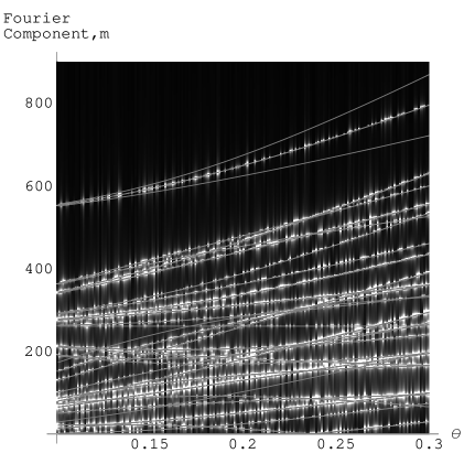
Figure 6: The Fourier transform of $\left|\langle i|U^{m}|\Psi\rangle\right|^{2}$,$F_{m,2048}$, is shown as a vertical density, as function of the horizontal co-ordinate $\theta$, for a fixed $\chi=0.2$, and 4 qubits. 4 qubits are chosen so as to provide a complex, but not confusing diagram. The white bands indicate a large Fourier component. The superimposed grey lines show all energy differences - note that some of these are disallowed. In this case, $2048$ samples are used in the Fourier series, and simulations are taken in steps of $0.01$ in $\theta$. From this diagram, we can see the energy gap between the ground state and first excited state approaching zero. We can also see a level crossing, where one of the grey lines is reflected through the origin at $\theta\simeq 0.25$.

One could change the value of $\frac{\theta}{\chi}$ over many experiments to tune the system through the critical coupling. In the thermodynamic limit, the energy gap to the first excited state would vanish at criticality, but we see in Fig. 5 that the condition is not strictly met for a finite number of qubits.

One can use this to show that the energy gap, $\Delta$, for the excitation from the ground to first excited state obeys the relation

$$\Delta\sim\left|\phi-\phi_{c}\right|^{\gamma}$$ (104)

with $\gamma=1$, as we expect from a standard treatment of the transverse Ising problemSachdev (2000).

III.3.1 Controlled-U Spectroscopy

The above method requires knowledge of the approximate values of $\left|\langle i|U^{m}|\Psi\rangle\right|^{2}$, which means that a measurement with result $|i\rangle$ must be achieved multiple times. In work by Miquel et al.Miquel et al. (2002), it has been shown that spectroscopy can be achieved much more easily by implementing a controlled-U gate, and measuring only a single qubitKnill and Laflamme (1998). We can achieve this by using an ancillary qubit, and express the controlled-U operation as

$$CU:\langle i|\otimes\langle\Psi|\rightarrow\langle i|\otimes U^{i}\langle\Psi|$$

where $\langle i|$ can be either $\langle 0|$, which takes $\langle\Psi|$ to $\langle\Psi|$, or $\langle 1|$, which takes $\langle\Psi|$ to $U\langle\Psi|$.

If we do a weak measurement on the control bit, we yield the result

$$\left\langle\sigma_{z}\right\rangle=\Re\left[Tr(U\rho)\right] \left\langle\sigma_{y}\right\rangle=\Im\left[Tr(U\rho)\right]$$ ,

where $\rho$ is the density matrix corresponding to the state has been prepared in. If we prepare it in the mixed state given by $\rho=I/2^{n}$ where $I$ is the identity operator, we yield $\left\langle\sigma_{z}\right\rangle=\Re\left[Tr(U)\right]/N$, which is proportional to the sum of the eigenvalues of $U$. If we repeat this for $U^{m}$ for a variety of $m$, we can use the method above to reconstruct the energy level diagram.

Further, Miquel et al.Miquel et al. (2002) propose a scheme using the quantum Fourier transform to probe specific regions of the spectrum of the eigenvalues of $U$. This is achieved by introducing an effective time scale into $U$, and exploiting the conjugacy of energy and time.

III.4 Phase Estimation Algorithm

In work done by Abrams and LloydAbrams and Lloyd (1999), and further explored in an ion trap context by Travaglione and MilburnTravaglione and Milburn (2002), it has been shown that it is possible to estimate the eigenvalues associated with any unitary transformation, $U$. These correspond directly to the energy eigenvalues of the equivalent Hamiltonian, which we are interested in. The scheme also yields an approximate eigenvector with high probability.

Starting with a mixed index state $|j\rangle_{I}$, and the state of the target system $|\Psi\rangle$, we perform the transformation

$$\Lambda(U):|j\rangle_{I}|\Psi\rangle_{T}\rightarrow|j\rangle_{I}\otimes U^{j}|\Psi\rangle_{T}$$

followed by a Fourier transformation on the index register. Measuring the index register will then yield, with high probability, an approximate eigenvector of $U$ in the target state, and information about the phase of the eigenvalue of $U$ in the index register.

Note, however, that use is made of an index register, which is at least the same size as the system of interest. This makes it a much more difficult problem to conquer experimentally, as a system twice as big will be much more prone to decoherence. In ion trap implementations, trapping twice as many ions will also be more difficult. While this technique is superior to the spectroscopic measurements suggested in the previous section, scalability issues may keep it from being experimentally feasible for some time.

IV Conclusion

We have presented a number of key ideas which will drive our search for a quantum phase transition in a system which is implementable on an ion-trap quantum computer in a natural way.

We have taken the Feynman thesis and turned it around, to ask what might happen if we have some implementable unitary transformation. The two fields which will help to answer this question have been introduced - namely, the ion-trap quantum architecture which will provide our unitary transformation, and the tools of renormalization group theory. In this paper, we have shown that the Hamiltonian corresponding to a separated Ising map belongs to the same universality class as the transverse Ising model. Further, the map presented here is realisable in a very natural way on an ion-trap quantum computing architecture.

We have also suggested some experimental signatures , including ground state energy and entanglement, and spectroscopic information which may lead to the reconstruction of the energy spectrum.

After completion of this work, we became aware of some other work on simulating quantum phase transitions in ion trapsPorras and Cirac (2004)