Quantum-“classical” correspondence in a nonadiabatic-transition system

Abstract

A nonadiabatic-transition system which exhibits “quantum chaotic” behavior [Phys. Rev. E 63, 066221 (2001)] is investigated from quasi-classical aspects. Since such a system does not have a naive classical limit, we take the mapping approach by Stock and Thoss [Phys. Rev. Lett. 78, 578 (1997)] to represent the quasi-classical dynamics of the system. We numerically show that there is a sound correspondence between the quantum chaos and classical chaos for the system.

Nonadiabatic transition (NT) is a very fundamental concept in physics and chemistry Nakamura02 ; TAWM00 . In atomic, molecular, and chemical physics literature, NTs occur as a breakdown of the Born-Oppenheimer (BO) approximation, which is essentially an adiabatic approximation to solve quantum systems with many degrees of freedom. It is still a tough problem to analyze the properties of NTs especially for multidimensional systems. One reason preventing us from deeper understanding of NT is the lack of a naive quantum-classical correspondence for NT like tunneling phenomena UT96 ; SI98 . One way to get the classical picture for a NT system is to go back to the original system before the BO approximation: Fuchigami and Someda investigated dynamical properties of H${}^{+}_{2}$ from classical points of view by treating an electron and nuclei as dynamical variables FS03 . Though there is a full quantum study for such a small system to compare with KKF99 , this “purist” way cannot be easily applied to much more “complex” systems.

The mapping method recently advocated by Stock and Thoss ST97 can circumvent this deficiency. (This is reminiscent of the Meyer-Miller method MM79 .) Their method is as follows: After the BO approximation, the discrete electronic degrees of freedom are mapped onto the Schwinger bosons JJSakurai . Since all the degrees of freedom become just bosons, the total system is rather easily treated semiclassically or quasi-classically. Using this method semiclassically, one can obtain, e.g., absorption spectra even for a pyrazin molecule with 24 degrees of freedom TMS00 . One can use it quasi-classically by solving the equations of motion derived from a mapping Hamiltonian. This is a very easy way to simulate NT systems because the additional number of degrees of freedom for electronic parts is rather small. Using the periodic orbit theory Gutzwiller90 or the adiabatic switching method Reinhardt90 , one can obtain even quantum eigenenergies and eigenstates, in principle ZGE86 .

On the other hand, multidimensional NT systems like Jahn-Teller molecules KDC84 are known to show “quantum chaotic” behavior Gutzwiller90 . Fujisaki and Takatsuka investigated this problem deeply employing the two-mode-two-state (TMTS) system which is considered as a system with two vibrational modes and two electronic states FT01b . They calculated the statistical properties of the eigenenergies and eigenfunction for the TMTS system, and found that the system becomes strongly “quantum chaotic” under a certain condition. In addition, they showed that the chaos is not just a reflection of the lower adiabatic system nor that of the diabatic systems. (On the other hand, the chaos of all previous studies is just a reflection of the lower adiabatic systems KDC84 .) This means that conventional classical descriptions do not help to explain the quantum chaotic behavior. Hence this system deserves to be further studied from the “mapping” (extended classical) points of view. Though there are some studies which investigated chaotic properties of this kind of mixed quantum-classical systems BE94 , our focus here is a quantum-“classical” correspondence (if any) for the TMTS system.

The TMTS system FT01b first introduced by Heller Heller90 is described by the following Hamiltonian:

$${\cal H}_{\rm TMTS}=\left(\begin{array}[]{cc}T_{{\rm kin}}+V_{A}&J\\ J&T_{{\rm kin}}+V_{B}\end{array}\right),$$ (1)

where $T_{\rm kin}$ is the kinetic energy, $V_{i}$ ($i=A,B$) is the potential energy for state $i$ defined by

$$T_{{\rm kin}} = \frac{1}{2}(p_{x}^{2}+p_{y}^{2}),$$ (2)

$$V_{A} = \frac{1}{2}(\omega_{x}^{2}x^{2}+\omega_{y}^{2}y^{2})+\epsilon_{A},$$ (3)

$$V_{B} = \frac{1}{2}(\omega_{x}^{2}\xi^{2}+\omega_{y}^{2}\eta^{2})+\epsilon_{B},$$ (4)

with

$$\xi = (x+2a\sin\theta)\cos 2\theta+(y-2a\cos\theta)\sin 2\theta,$$ (5)

$$\eta = -(x+2a\sin\theta)\sin 2\theta+(y-2a\cos\theta)\cos 2\theta.$$ (6)

Note that we have just used a harmonic potential for each state. For the geometrical meaning of the parameters, see Fig. 1.

Figure 1: A shematic representation of the TMTS system. The distance between the minima of the potential is $2a$, and the angle between the relevant crossing seam (dotted line) and the primary axis of each potential (dashed line) is $\theta$. Inset: The perspective of the TMTS system. The potential minima are different with $\Delta\epsilon=\epsilon_{B}-\epsilon_{A}=0.173$.

Here the Duschinsky angle $\theta$ TLL03 and the nonadiabatic coupling constant $J$ are two important parameters for the system. If these are appropriately chosen, the system becomes strongly “quantum chaotic”, i.e., the nearest-neighbor energy-level spacing distribution becomes the Wigner type and the amplitude distribution of the eigenstates becomes Gaussian FT01b .

The mapping Hamiltonian ST97 ; TMS00 for this system is

$$H_{\rm map}=T_{\rm kin}+N_{A}V_{A}+N_{B}V_{B}+J(x_{A}x_{B}+p_{A}p_{B})$$ (7)

with

$$N_{i}=\frac{x_{i}^{2}+p_{i}^{2}}{2}-\gamma\quad(i=A,B).$$ (8)

Note that $N_{A}+N_{B}=1$. From this relation, one might consider $N_{i}$ ($i=A,B$) as a probability but it is not the case. This is because the numerical range for $N_{i}$ is $-\gamma<N_{i}<1+\gamma$. The equations of motion for this Hamiltonian are derived as follows:

$$\frac{d}{dt}x_{A} = V_{A}p_{A}+Jp_{B},\quad\frac{d}{dt}p_{A}=-V_{A}x_{A}-Jx_{B},$$ (9)

$$\frac{d}{dt}x_{B} = V_{B}p_{B}+Jp_{A},\quad\frac{d}{dt}p_{B}=-V_{B}x_{B}-Jx_{A},$$ (10)

$$\frac{d}{dt}x = p_{x},\quad\frac{d}{dt}p_{x}=-\frac{\partial V_{A}}{\partial x}N_{A}-\frac{\partial V_{B}}{\partial x}N_{B},$$ (11)

$$\frac{d}{dt}y = p_{y},\quad\frac{d}{dt}p_{y}=-\frac{\partial V_{A}}{\partial y}N_{A}-\frac{\partial V_{B}}{\partial y}N_{B}.$$ (12)

As a reference system, we take the lower adiabatic system as in FT01b . The lower adiabatic systems is defined by the following Hamiltonian:

$$H^{-}_{\rm ad}=T_{\rm kin}+V_{\rm ad}^{-},$$ (13)

with

$$V_{\rm ad}^{-}=\frac{V_{A}+V_{B}}{2}-\sqrt{\left(\frac{V_{A}-V_{B}}{2}\right)^{2}+J^{2}}$$ (14)

Since the TMTS system can be quantum chaotic as mentioned above, we investigate the chaotic properties for the mapping system and the lower adiabatic system. As an indicater of chaos, it is very natural to take Lyapunov exponents Ott02 . We focus on a finite-time maximum Lyapunov exponent calculated as

$$\lambda_{\rm max}(T)\simeq\frac{1}{T}\log\frac{\Delta d(T)}{\Delta d(0)}$$ (15)

with

$$\Delta d(t)^{2} = \Delta\tilde{x}_{A}(t)^{2}+\Delta\tilde{p}_{A}(t)^{2}+\Delta\tilde{x}_{B}(t)^{2}+\Delta\tilde{p}_{B}(t)^{2}$$ (16)

$$+ \Delta\tilde{x}(t)^{2}+\Delta\tilde{p}_{x}(t)^{2}+\Delta\tilde{y}(t)^{2}+\Delta\tilde{p}_{y}(t)^{2}$$

where $\tilde{x}_{A}=x_{A}/\sqrt{2+2\gamma},\quad\tilde{p}_{A}=p_{A}/\sqrt{2+2\gamma},\quad\tilde{x}_{B}=x_{A}/\sqrt{2\gamma},\quad\tilde{p}_{B}=p_{A}/\sqrt{2\gamma},\quad\tilde{x}=\omega_{x}x/\sqrt{2E},\quad\tilde{y}=\omega_{y}y/\sqrt{2E},\quad\tilde{p}_{x}=p_{x}/\sqrt{2E},\quad\tilde{p}_{y}=p_{y}/\sqrt{2E},$ and $E$ is the total energy for the system. Here tilde variables are introduced for normalization and $\Delta$ means a distance between a trajectory and its auxiliary one. In the following we take the typical value of $\gamma$, i.e., $\gamma=1/2$ ST97 . For the numerical calculation of Lyapunov exponents, the method by Benettin et al. BGS76 is employed, i.e., we calculate $\lambda_{\rm max}(T)$ for a finite $T$, then shorten the distance $\Delta d(T)$ to $\Delta d(0)$, and run the trajectory again and so on. In this study, we took $T=24$ because of the numerical divergence of the $\Delta d(T)$ for larger values of $T$.

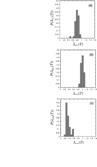
Figure 2: $J$ dependence of the distribution of the Lyapunov exponents for the mapping system. The nonadiabatic coupling is (a) $J=0.3$, (b) $J=1.5$, and (c) $J=7.5$. The finite time is $T=24$, and the iterative number of the time average is 10. The Duschinsky angle is $\theta=\pi/3$.

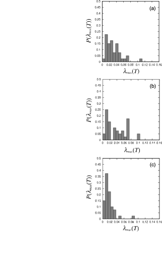
Figure 3: $J$ dependence of the distribution of the Lyapunov exponents for the lower adiabatic system. The nonadiabatic coupling is (a) $J=0.3$, (b) $J=1.5$, and (c) $J=7.5$. The finite time is $T=24$, and the iterative number of the time average is 10. The Duschinsky angle is $\theta=\pi/3$.

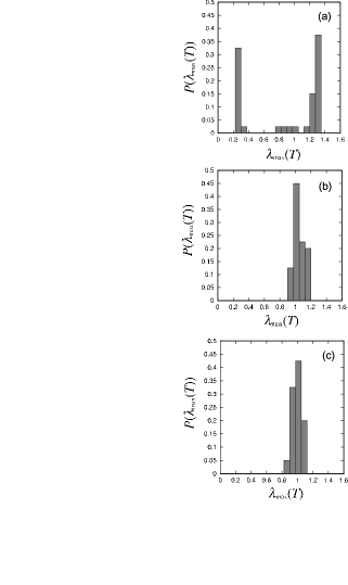
Figure 4: $\theta$ dependence of the phase space averaged Lyapunov exponent for the mapping system with $J=1.5$. The Duschinsky angle is (a) $\theta=0.0$, (b) $\theta=\pi/6$, and (c) $\theta=\pi/3$. The finite time is $T=24$, and the iterative number of the time average is 10.

Following the previous studies FT01b , we concentrate on a rather high energy region around $E=E_{0}=28$. (This energy is much higher than that around the crossing seam region.) Varying the Duschinsky angle $\theta$ and the nonadiabatic coupling constant $J$, we calculate the distribution of the finite-time maximum Lyapunov exponent $\lambda_{\rm max}(T)$. For simplicity, hereafter, we call $\lambda_{\rm max}(T)$ just as a Lyapunov exponent. Since the phase space has a structure especially for the lower adiabatic system, globally averaged Lyapunov exponents are not so useful. Instead, we investigate the properties of the distribution of the Lyapunov exponents, which reflects phase space structure of the system. (Remember that the Berry-Robnik distribution, which reflects the phase space volume of chaotic seas, is useful for mixed systems MHA01 .) To this end, we prepare an initial ensemble of particles which are sampled from a part of the equi-energy potential surface $V_{A}(x,y)=E_{0}$ with constraints $p_{x}=p_{y}=0$ and $y<x\tan\theta+a/\cos\theta$. (The latter constraint means that we only take points below the crossing seam. See Fig. 1.) We take 40 sample points from this curve and calculate the histogram for the Lyapunov exponents. We believe that these sample points represent a typical situation of the TMTS system because, at least, the characteristic of the lower adiabatic system can be understood from these sampling points FT01b .

First we fix $\theta=\pi/3$, and investigate the $J$ dependence of the chaotic properties. Let us summarize the corresponding quantum results: the nearest-neighbor (energy-level) spacing distribution is Wigner for $J=1.5$ (3rd row of Fig. 3 in FT01b ), whereas it is rather Poisson for $J=7.5$ (3rd row of Fig. 4 in FT01b ), and rather mixed for $J=0.3$ (3rd row of Fig. 2 in FT01b ). Figure 2 shows the distribution of the Lyapunov exponents for the TMTS system. The distribution for $J=1.5$ has a sharp peak around 1, whereas that for $J=7.5$ has a rather broad peak around 0.4, and that for $J=0.3$ is also a little bit broad. This corresponds to the quantum results, at least, qualitatively. On the other hand, Fig. 3 shows the distribution of the Lyapunov exponents for the lower adiabatic system. As one can see, the values themselves are much smaller than those for the TMTS system and it is difficult to distinguish three distributions. This also corresponds to the quantum mechanical calculation for the lower adiabatic system (Fig. 9 in FT01b ). From this comparison, it is reasonable to conclude that there is a sound quantum-“classical” correspondence between the TMTS system and the mapped system in view of their “chaotic” properties.

Next we investigate the $\theta$ dependence of the chaotic properties while fixing $J=1.5$. Although there is a strong peak around $\lambda_{\rm max}(T)\simeq 1.3$ as shown in Fig. 4 (a), we can see that the system with $\theta=0$ is not globally chaotic. This is because $x$ does not effectively coupled to $y$ when $\theta=0$, and the motion along $x$ axis is regular. (On the other hand, even with $\theta=0$, the motion along $y$ axis can be chaotic as shown by the peak of the distribution around 1.3.) In such a case, we do not expect that the Wigner type distribution arises in the corresponding quantum system, and this is the case for the TMTS system (1st row of Fig. 3 in FT01b ). On the other hand, for intermediate Duschinsky angles ($\theta=\pi/6,\pi/3$), the Lyapunov exponent distributions show that the system is globally chaotic [Fig. 4 (b),(c)], and the corresponding quantum system can have the Wiger type distribution, which is also confirmed numerically (2nd and 3rd rows of Fig. 3 in FT01b ). Of course, we have to admit that this correspondence is loosely stated, and there remains a difficult question exactly when the quantum chaos begins in the parameter space. Such an issue must be addressed utilizing semiclassical methods ST97 ; Gutzwiller90 or the adiabatic switching method Reinhardt90 . It is also interesting to investigate phase space structure of this mapping system and to relate it to the nearest-neighbor spacing distribution via the Berry-Robnik distribution MHA01 . We also hope that this study will cast a light on the relation between the statistical reaction theory for NT systems and Lyapunov spectra for them.

In this paper, employing the mapping approach by Stock and Thoss, we investigated a nonadiabatic-transition system which exhibits “quantum chaotic” behavior from quasi-classical aspects. By comparing the statistical properties of the quantum system with the Lyapunov exponent distributions of the mapping system, we found that there is a sound quantum-“classical” correspondence in the system.

The author thanks T. Takami for comments.

References

- (1) H. Nakamura, Nonadiabatic Transition: Concepts, Basic Theories and Applications (World Scientific, Singapore, 2002); C. Zhu, Y. Teranishi, and H. Nakamura, Adv. Chem. Phys. 117, 127 (2001).
- (2) K. Takatsuka, Y. Arasaki, K. Wang, and V. McKoy, Faraday Discuss. 115, 1 (2000); Y. Arasaki, K. Takatsuka, K. Wang, and V. McKoy, Phys. Rev. Lett. 90, 248303 (2003).
- (3) H. Ushiyama and K. Takatsuka, Phys. Rev. E 53, 115 (1996); K. Giese, H. Ushiyama, and O. Kühn, Chem. Phys. Lett. 371, 681 (2003).
- (4) A. Shudo and K.S. Ikeda, Physica D 115, 234 (1998); T. Onishi, A. Shudo, K.S. Ikeda, and K. Takahashi Phys. Rev. E 64, 025201(R) (2001).
- (5) S. Fuchigami and K. Someda, J. Phys. Soc. Jpn. 72, 1891 (2003). See also M. P. Strand and W. P. Reinhardt, J. Chem. Phys. 70, 3812 (1979).
- (6) I. Kawata, H. Kono, and Y. Fujimura, J. Chem. Phys. 110, 11152 (1999).
- (7) G. Stock and M. Thoss, Phys. Rev. Lett. 78, 578 (1997); M. Thoss and G. Stock, Phys. Rev. A 59, 64 (1999).
- (8) H.-D. Meyer and W. H. Miller, J. Chem. Phys. 70, 3214 (1979); ibid. 71, 2156 (1979). See also X. Sun and W. H. Miller, ibid. 106, 6346 (1997).
- (9) J.J. Sakurai, Modern Quantum Mechanics (Addison-Wesley, Reading, MA, 1994).
- (10) M. Thoss, W.H. Miller, and G. Stock, J. Chem. Phys. 112, 10282 (2000).
- (11) M. C. Gutzwiller, Chaos in Classical and Quantum Mechanics (Springer-Verlag, New York, 1990).
- (12) W. P. Reinhardt, Adv. Chem. Phys. 73, 925 (1990); R.T. Skodje and J.R. Cary, Comp. Phys. Rep. 8, 223 (1988).
- (13) J. Zwanziger, E.R. Grant, and G.S. Ezra, J. Chem. Phys. 85, 2089 (1986); M. Pletyukhov, Ch. Amann, M. Mehta, and M. Brack, Phys. Rev. Lett. 89, 116601 (2002); B. Balzer, S. Dilthey, S. Hahn, M. Thoss, and G. Stock, J. Chem. Phys. 119, 4204 (2003).
- (14) H. Köppel, W. Domcke, and L.S. Cederbaum, Adv. Chem. Phys. 57, 59 (1984); D.M. Leitner, H. Köppel, and L.S. Cederbaum, J. Chem. Phys. 104, 434 (1996); H. Yamasaki, Y. Natsume, A. Terai, and K. Nakamura, Phys. Rev. E 68, 046201 (2003).
- (15) H. Fujisaki and K. Takatsuka, Phys. Rev. E 63, 066221 (2001). See also H. Fujisaki and K. Takatsuka, J. Chem. Phys. 114, 3497 (2001); H. Higuchi and K. Takatsuka, Phys. Rev. E 66, 035203(R) (2002).
- (16) R. Blümel and B. Esser, Phys. Rev. Lett. 72, 3658 (1994); A. Bulgac and D. Kusnezov, Chaos, Solitions, and Fractals, 5, 1051 (1995); J. Gong and P. Brumer, Phys. Rev. Lett. 88, 203001 (2002).
- (17) E.J. Heller, J. Chem. Phys. 92, 1718 (1990).
- (18) See J. Tang, M.T. Lee, and S.H. Lin, J. Chem. Phys. 119, 7188 (2003), and references therein.
- (19) E. Ott, Chaos in Dynamical Systems, 2nd edition (Cambridge Univ. Press, Cambridge, 2002).
- (20) G. Benettin, L. Galgani, and J. Strelcyn, Phys. Rev. A 14, 2338 (1976). For recent accurate methods to calculate Lyapunov exponents, see T. Okushima, Phys. Rev. Lett. 91, 254101 (2003).
- (21) M.V. Berry and M. Robnik, J. Phys. A 17, 2413 (1984); H. Makino, T. Harayama, and Y. Aizawa, Phys. Rev. E 63, 056203 (2001).