Violation of the Nernst heat theorem in the theory of thermal Casimir force between Drude metals

Abstract

We give a rigorous analytical derivation of low-temperature behavior of the Casimir entropy in the framework of the Lifshitz formula combined with the Drude dielectric function. An earlier result that the Casimir entropy at zero temperature is not equal to zero and depends on the parameters of the system is confirmed, i.e. the third law of thermodynamics (the Nernst heat theorem) is violated. We illustrate the resolution of this thermodynamical puzzle in the context of the surface impedance approach by several calculations of the thermal Casimir force and entropy for both real metals and dielectrics. Different representations for the impedances, which are equivalent for real photons, are discussed. Finally, we argue in favor of the Leontovich boundary condition which leads to results for the thermal Casimir force that are consistent with thermodynamics.

I Introduction

During the last few years the Casimir effect 1 has attracted a lot of experimental and theoretical attention as a nontrivial macroscopic evidence for the existence of zero-point oscillations of electromagnetic field (see, e.g., monographs 2 ; 3 ; 4 and reviews 5 ; 6 ). Except for calculations of the Casimir force between perfectly shaped bodies made of ideal metal at zero temperature, the topical studies were conducted taking into account the effects of surface roughness, finite conductivity of the boundary metal and nonzero temperature 6 .

The correct theoretical description of the thermal Casimir force between real metals has assumed great importance due to recent precision experiments 7 ; 8 ; 9 ; 10 ; 11 ; 12 ; 13 ; 14 ; 15 ; 16 , followed by the prospective applications of the Casimir effect in nanotechnology 17 ; 18 and also its use as a test for predictions of fundamental physical theories 16 ; 19 ; 20 ; 21 ; 22 ; 23 . It was found unexpectedly that the calculations of the thermal Casimir force between two parallel plates made of real metal based on the Lifshitz formula 24 supplemented by some model dielectric function ran into serious difficulties. The key question of the controversy is whether the transverse electric zero mode contributes to the Casimir effect in the case of real metals. In Refs. 25 ; 26 a positive answer to this question was obtained by the substitution of the plasma dielectric function into the Lifshitz formula. In the limit of infinitely high conductivity the results of Ref. 25 ; 26 are smoothly transformed into the familiar results for ideal metals 6 . In Ref. 27 the Drude dielectric function was used to calculate the contributions of both longitudinal and transverse modes to the Casimir force. It was found that the transverse electric zero mode does not contribute 27 . The results of Ref. 27 do not smoothly join with those for ideal metals. In the high-temperature limit, where the contribution of the zero modes is dominant, the Casimir force between plates made of Drude metals proves to be equal to one half of the force between the ideal metals. Today, there is an extensive literature on these two and other approaches to the calculation of the thermal Casimir force between real metals 25 ; 26 ; 27 ; 28 ; 29 ; 30 ; 31 ; 32 ; 32a ; 33 ; 34 ; 35 ; 36 ; 37 ; 38 ; 38a .

From this discussion it has been shown 38 that the substitution of the Drude dielectric function into the Lifshitz formula results in negative values of the Casimir entropy within wide temperature interval and leads to the violation of the third law of thermodynamics (the Nernst heat theorem). On the contrary, Refs. 31 ; 32 ; 32a have thrown doubt on the computations of Ref. 38 and presented the numerical computations in favor of the statement that the Casimir entropy for the Drude metals is zero at zero temperature, i.e. the third law of thermodynamics is not violated.

In the present paper we give a detailed and rigorous analytical derivation of the low-temperature behavior of the Casimir entropy in the framework of the Lifshitz formula combined with the Drude dielectric function (Sec. II). This derivation removes the doubts raised in Refs. 31 ; 32 ; 32a and validates the thermodynamic inconsistency of the Drude dielectric function with the Lifshitz formula at nonzero temperature. The reason why the opposite conclusion is obtained in Refs. 31 ; 32 ; 32a is explained in Sec. III. This section contains also the resolution of the above thermodynamic puzzle by presenting several computations in the framework of the surface impedance approach 35 ; 36 as opposed to the use of the Drude model. The exact boundary conditions in terms of impedances, depending on polarization and angle of incidence, are compared with the Leontovich boundary condition. The latter is shown to be applicable to the case of fluctuating fields being in agreement with the third law of thermodynamics. The temperature dependences of the Casimir force and entropy for real metals in both approaches are compared with those for dielectrics. Sec. IV contains conclusions and discussion of recent experimental results.

II Casimir free energy and entropy in the Lifshitz theory combined with the Drude model

The Casimir free energy for the configuration of two parallel plates at a separation $a$ and temperature $T$ is given by the Lifshitz formula 24 , which can be represented in the form

$${\cal{F}}(a,T)=\frac{k_{B}T}{8\pi a^{2}}\sum\limits_{l=0}^{\infty}{\vphantom{\sum}}^{\prime}\int_{\zeta_{l}}^{\infty}ydy\left\{\ln\left[1-r_{\|}^{2}(\zeta_{l},y)e^{-y}\right]+\ln\left[1-r_{\bot}^{2}(\zeta_{l},y)e^{-y}\right]\right\}.$$ (1)

Here prime adds a multiple 1/2 near the term with $l=0$, $k_{B}$ is the Boltzmann constant, the dimensionless Matsubara frequencies are $\zeta_{l}=\xi_{l}/\omega_{c}$, where $\xi_{l}=2\pi k_{B}Tl/\hbar$, $\omega_{c}=c/(2a)$, and the reflection coefficients for the two different polarizations are expressed in terms of the dielectric permittivity $\varepsilon(\omega)$ as

$$r_{\|}^{2}(\zeta_{l},y)=\left\{\frac{y\varepsilon(i\zeta_{l})-\sqrt{\left[\varepsilon(i\zeta_{l})-1\right]\zeta_{l}^{2}+y^{2}}}{y\varepsilon(i\zeta_{l})+\sqrt{\left[\varepsilon(i\zeta_{l})-1\right]\zeta_{l}^{2}+y^{2}}}\right\}^{2},$$

$$r_{\bot}^{2}(\zeta_{l},y)=\left\{\frac{y-\sqrt{\left[\varepsilon(i\zeta_{l})-1\right]\zeta_{l}^{2}+y^{2}}}{y+\sqrt{\left[\varepsilon(i\zeta_{l})-1\right]\zeta_{l}^{2}+y^{2}}}\right\}^{2}.$$ (2)

We consider the Drude metals described by the dielectric permittivity of the Drude model. At the imaginary Matsubara frequencies it is given by

$$\varepsilon^{(D)}(i\zeta_{l})=1+\frac{{\tilde{\omega}}_{p}^{2}}{\zeta_{l}\left[\zeta_{l}+{\tilde{\gamma}}(T)\right]},$$ (3)

where ${\tilde{\omega}}_{p}$ and ${\tilde{\gamma}}(T)$ are the dimensionless plasma frequency and relaxation parameter defined by ${\tilde{\omega}}_{p}=\omega_{p}/\omega_{c}$, ${\tilde{\gamma}}(T)=\gamma(T)/\omega_{c}$. In the absence of relaxation ${\tilde{\gamma}}(T)=0$ and $\varepsilon^{(D)}$ coincides with the dielectric permittivity of the free electron plasma model $\varepsilon^{(p)}$. Substituting Eq. (3) into Eqs. (1), (2) one obtains the Casimir free energy ${\cal{F}}^{(D)}(a,T)$ and the reflection coefficients $r_{\|,\bot}^{(D)}(\zeta_{l},y)$ in the framework of the Drude model. If, from the very beginning, $\gamma(T)=0$, then the Casimir free energy in the framework of the plasma model ${\cal{F}}^{(p)}(a,T)$ and reflection coefficients $r_{\|,\bot}^{(p)}(\zeta_{l},y)$ are obtained. It is notable that $r_{\bot}^{(D)}(0,y)=0$, whereas

$${r_{\bot}^{(p)}}^{2}(0,y)={r_{\bot}^{(p)}}^{2}(\zeta_{l},y)=\left(\frac{y-\sqrt{{\tilde{\omega}}_{p}^{2}+y^{2}}}{y+\sqrt{{\tilde{\omega}}_{p}^{2}+y^{2}}}\right)^{2}\neq 0,$$ (4)

i.e. there is no smooth transition from ${\cal{F}}^{(D)}$ to ${\cal{F}}^{(p)}$ when $\gamma(T)\to 0$. This nonanalyticity is determined exclusively by the zero-frequency contribution of the transverse electric mode to the free energy ${\cal{F}}^{(D)}(a,T)$.

For the calculation of the Drude free energy ${\cal{F}}^{(D)}(a,T)$ it is useful to represent it as the plasma free energy ${\cal{F}}^{(p)}(a,T)$ plus some additional terms. Taking into account that $r_{\bot}^{(D)}(0,y)=0$ and ${r_{\|}^{(p)}}^{2}(0,y)={r_{\|}^{(D)}}^{2}(0,y)=1$, this identical representation is as follows

$${\cal{F}}^{(D)}(a,T)={\cal{F}}^{(p)}(a,T)-\frac{k_{B}T}{16\pi a^{2}}\int_{0}^{\infty}ydy\ln\left[1-{r_{\bot}^{(p)}}^{2}(0,y)e^{-y}\right]$$ (5)

$$\phantom{aaa}+\frac{k_{B}T}{8\pi a^{2}}\sum\limits_{l=1}^{\infty}{\vphantom{\sum}}^{\prime}\int_{\zeta_{l}}^{\infty}ydy\left\{\ln\left[1-{r_{\|}^{(D)}}^{2}(\zeta_{l},y)e^{-y}\right]-\ln\left[1-{r_{\|}^{(p)}}^{2}(\zeta_{l},y)e^{-y}\right]\right.$$

$$\phantom{aaaaaa}\left.+\ln\left[1-{r_{\bot}^{(D)}}^{2}(\zeta_{l},y)e^{-y}\right]-\ln\left[1-{r_{\bot}^{(p)}}^{2}(\zeta_{l},y)e^{-y}\right]\right\}.$$

An important point is that the zero-frequency contributions are contained only in the first two terms of the right-hand side of Eq. (5), whilst the summation starts from the term with $l=1$ leading to nonzero lower integration limits $\zeta_{l}$ in the integrals at any nonzero temperature.

It is instructive to find the asymptotic representation for the free energy (5) applicable at $T\to 0$. First we notice that among the three parameters, contained in Eq. (3), i.e ${\tilde{\omega}}_{p}$, $\zeta_{l}$ (with $l\geq 1$) and ${\tilde{\gamma}}(T)$, the latter is the smallest one. In fact at $T=300\,$K for good metals $\gamma\sim 10^{13}-10^{14}\,$rad/s (for Au $\gamma=5.32\times 10^{13}\,$rad/s) whereas $\xi_{1}=2\pi k_{B}T/\hbar=2.46\times 10^{14}\,$rad/s, and $\xi_{l}=l\xi_{1}$, i.e. in all cases $\gamma<\xi_{l}$. When $T$ decreases from room temperature up to approximately $T_{D}/4$, where $T_{D}$ is the Debye temperature ($T_{D}=165\,$K for Au 39 ), $\gamma(T)\sim T$, i.e. $\gamma(T)$ decreases following the same law as $\xi_{l}$, preserving the inequality $\gamma(T)<\xi_{l}$. At $T<T_{D}/4$ the relaxation parameter decreases even more quickly than $\xi_{l}$ with decreasing $T$ (as $\sim T^{5}$ according to the Bloch-Grüneisen law due to electron-phonon collisions 40 and as $\sim T^{2}$ at liquid helium temperatures due to electron-electron scattering 39 ). As a result, at $T=30\,$K $\gamma(T)/\xi_{1}(T)\approx 4.9\times 10^{-2}$, at $T=10\,$K $\gamma(T)/\xi_{1}(T)\approx 1.8\times 10^{-3}$, and this relation decreases further with $T\to 0$, i.e. at low temperatures the condition $\gamma(T)\ll\xi_{l}(T)$ is largely satisfied.

The largest parameter of the above three is $\omega_{p}$ (for Au $\omega_{p}=1.37\times 10^{16}\,$rad/s). For example, for Au at $T=300\,$K, 70 K, and 10 K we have $\gamma(T)/\omega_{p}={\tilde{\gamma}}(T)/{\tilde{\omega}}_{p}=3.88\times 10^{-3}$, $6.71\times 10^{-4}$, $1.06\times 10^{-6}$, respectively.

The reflection coefficients (2) have continuous derivatives with respect to the relation $\gamma(T)/\xi_{l}(T)$ ($l\geq 1$) at the point $\gamma(T)/\xi_{l}(T)=0$. Under the above proved condition $\gamma(T)\ll\xi_{l}(T)$, which is satisfied at all sufficiently low temperatures, the relation $\gamma(T)/\xi_{l}(T)\ll 1$, and we can expand in Taylor series around a point $\gamma(T)/\xi_{l}(T)=0$ keeping only the first order terms

$${r_{\|}^{(D)}}^{2}(\zeta_{l},y)={r_{\|}^{(p)}}^{2}(\zeta_{l},y)-\frac{{\tilde{\gamma}}(T)}{\zeta_{l}(T)}R_{\|}(\zeta_{l},y),$$

$${r_{\bot}^{(D)}}^{2}(\zeta_{l},y)={r_{\bot}^{(p)}}^{2}(\zeta_{l},y)-\frac{{\tilde{\gamma}}(T)}{\zeta_{l}(T)}R_{\bot}(\zeta_{l},y),$$ (6)

where

$$R_{\|}(\zeta_{l},y)=\frac{2\zeta_{l}^{2}\alpha y\left[1+\alpha^{2}\left(2y^{2}-\zeta_{l}^{2}\right)\right]|r_{\|}^{(p)}(\zeta_{l},y)|}{\sqrt{1+\alpha^{2}y^{2}}\left[y+\alpha\zeta_{l}^{2}\left(\alpha y+\sqrt{1+\alpha^{2}y^{2}}\right)\right]^{2}},$$

$$R_{\bot}(\zeta_{l},y)=\frac{2\alpha y|r_{\bot}^{(p)}(\zeta_{l},y)|}{\sqrt{1+\alpha^{2}y^{2}}\left(\alpha y+\sqrt{1+\alpha^{2}y^{2}}\right)^{2}},$$ (7)

and $\alpha\equiv 1/{\tilde{\omega}}_{p}=\lambda_{p}/(4\pi a)$, $\lambda_{p}$ is the plasma wavelength (note that we keep the argument $T$ when $\zeta_{l}$ participates in the expansion parameter but omit it in the other cases).

The same expansions for the logarithms which appear in Eq. (1) are

$$\ln\left[1-{r_{\|}^{(D)}}^{2}(\zeta_{l},y)e^{-y}\right]=\ln\left[1-{r_{\|}^{(p)}}^{2}(\zeta_{l},y)e^{-y}\right]+\frac{{\tilde{\gamma}}(T)}{\zeta_{l}(T)}\frac{R_{\|}(\zeta_{l},y)e^{-y}}{1-{r_{\|}^{(p)}}^{2}(\zeta_{l},y)e^{-y}},$$

(8)

$$\ln\left[1-{r_{\bot}^{(D)}}^{2}(\zeta_{l},y)e^{-y}\right]=\ln\left[1-{r_{\bot}^{(p)}}^{2}(\zeta_{l},y)e^{-y}\right]+\frac{{\tilde{\gamma}}(T)}{\zeta_{l}(T)}\frac{R_{\bot}(\zeta_{l},y)e^{-y}}{1-{r_{\bot}^{(p)}}^{2}(\zeta_{l},y)e^{-y}}.$$

Substituting Eq. (8) in Eq. (5) we obtain the following expression for the Casimir free energy between parallel plates made of Drude metal

$${\cal{F}}^{(D)}(a,T)={\cal{F}}^{(p)}(a,T)-\frac{k_{B}T}{16\pi a^{2}}\int_{0}^{\infty}ydy\ln\left[1-{r_{\bot}^{(p)}}^{2}(0,y)e^{-y}\right]+{\cal{F}}^{(\gamma)}(a,T),$$ (9)

where the contribution depending on the relaxation parameter is given by

$${\cal{F}}^{(\gamma)}(a,T)=\frac{{\tilde{\gamma}}(T)}{{\tilde{\omega}}_{p}}\frac{k_{B}T}{8\pi a^{2}}\sum\limits_{l=1}^{\infty}\frac{{\tilde{\omega}}_{p}}{\zeta_{l}(T)}\int_{\zeta_{l}}^{\infty}ydy\left[\frac{R_{\|}(\zeta_{l},y)}{e^{y}-{r_{\|}^{(p)}}^{2}(\zeta_{l},y)}+\frac{R_{\bot}(\zeta_{l},y)}{e^{y}-{r_{\bot}^{(p)}}^{2}(\zeta_{l},y)}\right].$$ (10)

Notice that in this expression the small parameter ${\tilde{\gamma}}(T)/{\tilde{\omega}}_{p}=\gamma(T)/\omega_{p}$, which does not depend on an index of summation, is put in evidence.

The low-temperature asymptotic limit of the Casimir free energy ${\cal{F}}^{(p)}(a,T)$ in the framework of the plasma model was investigated with details in Ref. 38 (the coinciding numerical results follow also from the computations of Ref. 25 ). In terms of the two small parameters $T/T_{eff}$ [where $k_{B}T_{eff}\equiv\hbar c/(2a)=\hbar\omega_{c}$] and $\delta_{0}/a=2\alpha$ [where $\delta_{0}=\lambda_{p}/(2\pi)$ is the skin layer thickness in the frequency region of the infrared optics] the plasma model free energy is given by 38

$${\cal{F}}^{(p)}(a,T)=E^{(p)}(a)-\frac{\hbar c\zeta(3)}{16\pi a^{3}}\left[\vphantom{\left[\left(\frac{T}{T_{eff}}\right)^{2}e^{2\pi T_{eff}/T}\right]}\left(1+2\frac{\delta_{0}}{a}\right)\left(\frac{T}{T_{eff}}\right)^{3}-\frac{\pi^{3}}{45\zeta(3)}\left(1+4\frac{\delta_{0}}{a}\right)\left(\frac{T}{T_{eff}}\right)^{4}\right],$$ (11)

where $E^{(p)}(a)$ is the Casimir energy at zero temperature calculated by using the plasma model dielectric function. The perturbation expansion (11) is applicable at separations $\lambda_{p}\leq a<3\,\mu$m at all temperatures $T\leq 300\,$K 26 .

The second term in the right-hand side of Eq. (9) is linear in the temperature. It is an easy matter to calculate the coefficient near $T$ perturbatively. For this purpose we use Eq.(4) and expand the logarithm under the integral in powers of $\delta_{0}/a$. Then all integrals are taken explicitly, resulting in

$$-\frac{k_{B}T}{16\pi a^{2}}\int_{0}^{\infty}ydy\ln\left[1-{r_{\bot}^{(p)}}^{2}(0,y)e^{-y}\right]=\frac{k_{B}T\zeta(3)}{16\pi a^{2}}\left\{\vphantom{O\left[\left(\frac{\delta_{0}}{a}\right)^{5}\right]}1-4\frac{\delta_{0}}{a}+12\left(\frac{\delta_{0}}{a}\right)^{2}\right.$$ (12)

$$\phantom{aaaa}\left.-32\left(\frac{\delta_{0}}{a}\right)^{3}\left[1-\frac{\zeta(5)}{16\zeta(3)}\right]+80\left(\frac{\delta_{0}}{a}\right)^{4}\left[1-\frac{\zeta(5)}{4\zeta(3)}\right]\right\},$$

where $\zeta(z)$ is the Riemann zeta function.

Now we consider the low-temperature behavior of the last term in the right-hand side of Eq. (9), ${\cal{F}}^{(\gamma)}(a,T)$, which depends on the relaxation parameter. An important point is that the relaxation parameter is not an independent one but is the function of the temperature, $\gamma=\gamma(T)$. Because of this, it is not improbable that the temperature dependent terms resulting from the integration and summation in Eq. (10) will cancel the second term, linear in the temperature, in the Casimir free energy (9). Below we demonstrate that this is not the case.

As pointed out above, $\gamma(T)\to 0$ when $T\to 0$ no slower than $\sim T^{2}$. If desired that the quantity ${\cal{F}}^{(\gamma)}(a,T)$ from Eq. (10) be linear in $T$, the sum in Eq. (10) should tend to infinity as $1/T^{2}$ when $T\to 0$. Let us find what is the actual asymptotic behavior of the quantity ${\cal{F}}^{(\gamma)}(a,T)$ when $T\to 0$. For this purpose we expand $R_{\|,\bot}(\zeta_{l},y)$ from Eq. (7) up to the first order in the small parameter $\alpha$ (recall that ${\cal{F}}^{(\gamma)}$ is already proportional to the smallest parameter of our problem $\gamma/\omega_{p}$)

$$R_{\|}(\zeta_{l},y)=\frac{2\zeta_{l}^{2}\alpha}{y},\qquad R_{\bot}(\zeta_{l},y)=2y\alpha.$$ (13)

Substituting Eq. (13) into Eq. (10) one obtains

$${\cal{F}}^{(\gamma)}(a,T)=\frac{\gamma(T)}{\omega_{p}}\frac{k_{B}T}{4\pi a^{2}}\sum\limits_{l=1}^{\infty}\left(\zeta_{l}\int_{\zeta_{l}}^{\infty}\frac{dy}{e^{y}-1}+\frac{1}{\zeta_{l}}\int_{\zeta_{l}}^{\infty}\frac{y^{2}dy}{e^{y}-1}\right).$$ (14)

Each of the two sums in Eq. (14) can be simply found when $T\to 0$. The asymptotic of the first sum is as follows

$$\sum\limits_{l=1}^{\infty}\zeta_{l}\int_{\zeta_{l}}^{\infty}\frac{dy}{e^{y}-1}=\frac{2\pi T}{T_{eff}}\sum\limits_{k=1}^{\infty}\frac{1}{k}\left[\frac{1}{e^{2\pi kT/T_{eff}}-1}+\frac{1}{\left(e^{2\pi kT/T_{eff}}-1\right)^{2}}\right]\approx\frac{T_{eff}}{2\pi T}\zeta(3)+\zeta(2)$$ (15)

(here we have neglected all terms in the expansion of $\exp(2\pi kT/T_{eff})$ in the denominators starting from the third ones). For the second sum in Eq.(14) one obtains

$$\sum\limits_{l=1}^{\infty}\frac{1}{\zeta_{l}}\int_{\zeta_{l}}^{\infty}\frac{y^{2}dy}{e^{y}-1}=\frac{T_{eff}}{2\pi T}\left[\vphantom{\frac{e^{2\pi kT/T_{eff}}}{\left(e^{2\pi kT/T_{eff}}-1\right)^{2}}}-2\sum\limits_{k=1}^{\infty}\frac{1}{k^{3}}\ln\left(1-e^{-2\pi kT/T_{eff}}\right)+\frac{4\pi T}{T_{eff}}\sum\limits_{k=1}^{\infty}\frac{1}{k^{2}}\frac{1}{e^{2\pi kT/T_{eff}}-1}\right.$$

(16)

$$\phantom{aaa}\left.+\frac{4\pi^{2}T^{2}}{T_{eff}^{2}}\sum\limits_{k=1}^{\infty}\frac{1}{k}\frac{e^{2\pi kT/T_{eff}}}{\left(e^{2\pi kT/T_{eff}}-1\right)^{2}}\right]\approx-\frac{T_{eff}\zeta(3)}{\pi T}\ln\frac{2\pi T}{T_{eff}}+\frac{3T_{eff}\zeta(3)}{2\pi T}+2\zeta(2).$$

Substituting Eqs. (15), (16) into Eq. (14) we arrive at

$${\cal{F}}^{(\gamma)}(a,T)\approx\frac{\gamma(T)}{\omega_{p}}\frac{k_{B}T_{eff}\zeta(3)}{4\pi^{2}a^{2}}\left[-\ln\frac{2\pi T}{T_{eff}}+2+3\pi\frac{\zeta(2)}{\zeta(3)}\frac{T}{T_{eff}}\right].$$ (17)

As is seen from Eq. (17), the leading term in ${\cal{F}}^{(\gamma)}(a,T)$ behaves as $-\gamma(T)\ln(T/T_{eff})$ and goes to zero when $T\to 0$ because $\gamma(T)\sim T^{2}$ at helium and lower temperatures.

Now we are in a position to find the low temperature behavior of the Casimir entropy

$$S^{(D)}(a,T)=-\frac{\partial{\cal{F}}^{(D)}(a,T)}{\partial T}$$ (18)

calculated by using the Drude dielectric function, where the Casimir free energy ${\cal{F}}^{(D)}(a,T)$ is given by Eq. (9). According to Eq. (9), there are three contributions into the Casimir entropy in the framework of the Drude model at low temperatures. The first one is given by the Casimir entropy calculated by means of the free electron plasma dielectric function. It is obtained from Eq. (11)

$$S^{(p)}(a,T)=-\frac{\partial{\cal{F}}^{(p)}(a,T)}{\partial T}=\frac{3k_{B}\zeta(3)}{8\pi a^{2}}\left(\frac{T}{T_{eff}}\right)^{2}$$ (19)

$$\phantom{aaa}\times\left\{1-\frac{4\pi^{3}}{135\zeta(3)}\frac{T}{T_{eff}}+2\frac{\delta_{0}}{a}\left[1-\frac{8\pi^{3}}{135\zeta(3)}\frac{T}{T_{eff}}\right]\right\}.$$

This result coincides with the one obtained in Ref. 38 (it is also in agreement with the numerical computations of the thermal corrections to the Casimir force in Refs. 25 ; 26 ). Evidently the plasma model Casimir entropy is positive and $S^{(p)}(a,T)\to 0$ when $T\to 0$, i.e. it is in agreement with the Nernst heat theorem.

The second contribution to the Drude model Casimir entropy is obtained from the second term in the right-hand side of Eq. (9) taking into account Eq. (12) and is given by

$$S_{0}^{(D)}(a,T)=S_{0}^{(D)}(a,0)=\frac{k_{B}}{16\pi a^{2}}\int_{0}^{\infty}ydy\ln\left[1-{r_{\bot}^{(p)}}^{2}(0,y)e^{-y}\right]$$

$$\phantom{aaaa}=-\frac{k_{B}\zeta(3)}{16\pi a^{2}}\left[1-4\frac{\delta_{0}}{a}+12\left(\frac{\delta_{0}}{a}\right)^{2}-\ldots\right]$$ (20)

[see Eq. (12) for higher perturbation orders in $\delta_{0}/a$]. This contribution is negative and does not depend on the temperature.

The asymptotic behavior of the last contribution to the Casimir entropy in the Drude model, as given by Eq. (9), at $T\to 0$, is obtained from Eq. (17) with account $\gamma(T)=\gamma_{0}T^{2}$

$$S^{(\gamma)}(a,T)=-\frac{\partial{\cal{F}}^{(\gamma)}(a,T)}{\partial T}\approx-\frac{k_{B}\zeta(3)}{4\pi^{2}a^{2}}\frac{\gamma(T)}{\omega_{p}}\frac{T_{eff}}{T}\left[-2\ln\frac{2\pi T}{T_{eff}}+3+9\pi\frac{\zeta(2)}{\zeta(3)}\frac{T}{T_{eff}}\right].$$ (21)

From Eq. (21) we notice that $S^{(\gamma)}(a,T)\to 0$ when $T\to 0$.

As a result, the value of the Casimir entropy at zero temperature calculated with the help of the Drude dielectric function is found from Eqs. (19)–(21):

$$S^{(D)}(a,0)=\lim\limits_{T\to 0}\left[S^{(p)}(a,T)+S_{0}^{(D)}(a,T)+S^{(\gamma)}(a,T)\right]=S_{0}^{(D)}(a,0)<0,$$ (22)

where the quantity in the right-hand side is negative and is given by Eq. (20). This quantity depends on the parameters of the system, such as the separation between the plates and plasma frequency, violating the third law of thermodynamics 41 ; 42 (the Nernst heat theorem). Therefore we may conclude that the Drude dielectric function is thermodynamically inconsistent with the Lifshitz formula and unusable to calculate the thermal Casimir force between real metals. Note also that according to Eqs. (20)–(22) the Casimir entropy between two parallel plates made of Drude metals is negative within a wide separation range. The entropy cannot be made positive by introducing some composite system containing a subsystem with negative entropy between the two infinite plates without changing the value of the Casimir force.

In the next section we discuss the possibilities to avoid the above thermodynamical puzzle and formulate the approach in which the Casimir entropy is positive, becoming zero at zero temperature.

III Towards a thermodynamically consistent theory of the thermal Casimir force between real metals

The above asymptotic limit for the Casimir entropy was derived under the important condition that $\gamma(T)\ll\xi_{l}(T)$, i.e. at any $T$ the magnitude of the relaxation parameter must be much less than the Matsubara frequencies. If this condition does not hold, the obtained conclusion concerning the thermodynamical inconsistency of the Drude model combined with the Lifshitz formula is open to question. This explains why in Refs. 31 ; 32 ; 32a it was concluded that the Lifshitz formula combined with the Drude model respects the Nernst heat theorem. In Refs. 31 ; 32 ; 32a all computations were performed under the condition that the relaxation parameter is constant (the values $\gamma=35.6\,$meV or 0.01 meV, as at $T=300\,$K and $T=10\,$K, respectively, were extended to all temperatures). Then even for the smaller value, at temperatures $T<0.018\,$K the inequality $\gamma>\xi_{1}(T)$ is fulfilled, i.e. the condition $\gamma(T)\ll\xi_{l}(T)$ is violated, and our proof in Sec. II is not applicable.

The question arises whether there are physical prerequisites for violating the condition $\gamma(T)\ll\xi_{l}(T)$. According to Sec. II, the nonelastic processes of electron-phonon collisions and also the elastic electron-electron scattering respect the inequality $\gamma(T)\ll\xi_{l}(T)$. One may hope, however, that some fine properties of real metal bodies could result in the violation of this inequality at some sufficiently low temperatures. It has been proposed 43 that this role can be played by impurities and defects which lead to a nonzero residual value of the static resistivity (and, thus, a relaxation parameter; recall that resistivity is proportional to the relaxation parameter 40 ) as the temperature goes to zero (see also Appendix D in Ref. 32 ).

Here we adduce the argument that impurities cannot remedy the situation with the violation of the Nernst heat theorem. In fact, the resistivity ratio of a sample can be defined as the ratio of its resistivity at room temperature to its residual resistivity. For pure samples the resistivity ratio may be as high as $10^{6}$ 39 . As an example, let us consider Au with $\gamma(T=300\,\mbox{K})=5.32\times 10^{13}\,$rad/s. In this case for the residual value of the relaxation parameter one obtains $\gamma_{res}=5.32\times 10^{7}\,$rad/s. The asymptotic expressions of Sec. II are applicable under the condition $\gamma\ll\xi_{1}=2\pi k_{B}T/\hbar$. Thus, with allowance made for impurities, these asymptotics are applicable at temperatures $T\gg\hbar\gamma_{res}/(2\pi k_{B})=6.5\times 10^{-5}\,$K. What this means is that the Casimir entropy at temperature $T=5\times 10^{-4}\,$K has a nonzero negative value given by Eq. (20). Physically this is equivalent to the violation of the Nernst heat theorem. Only at smaller temperatures of about $10^{-4}\,$K does Eq. (20) break down and the Casimir entropy rapidly takes a sharp upward turn to zero. We would like to point out also that the usual theory of the electron-phonon interaction, describing electrons interacting with elementary excitations of a perfect lattice with no impurities, must satisfy and does satisfy all the requirements of thermodynamics. In fact, the mean free path of the electrons between the collisions with impurities at zero temperature is many orders of magnitude greater than the penetration depth of the electromagnetic oscillations at the characteristic frequency into the metal. To make sure that this is the case, recall that the relaxation time for Au (the inverse of the relaxation parameter) at $T=300\,$K is equal to $\tau(T=300\,\mbox{K})=1.88\times 10^{-14}\,$s. Using the above resistivity ratio, one obtains the value of the relaxation time at zero temperature $\tau(T\approx 0\,\mbox{K})=1.88\times 10^{-8}\,$s. Finally, using the value of Fermi velocity for Au ($v_{F}=1.79\times 10^{6}\,$m/s) the mean free path of the electron is equal to $l(T\approx 0\,\mbox{K})=v_{F}\tau(T\approx 0\,\mbox{K})=3.36\,$cm. This should be compared with the thickness of the skin layer in the region of the infrared optics, equal to approximately 22 nm. That is why the attempt to remedy the violation of the Nernst heat theorem at the expense of impurities is meaningless.

Recently the resolution of these complicated problems was obtained 36 using another approach to the description of real metals based on the concept of the Leontovich impedance boundary conditions. This approach offers a fundamental understanding of the reason why the Drude model is not compatible with the theory of the thermal Casimir force between real metals.

The main concept of the Lifshitz theory is the fluctuating electromagnetic field considered on the background of dielectric permittivity depending only on frequency. This concept works good in the case of dielectrics but is not adequate for real metals. In fact, in the frequency region of the anomalous skin effect the spatial non-uniformity of the field makes impossible a description of a metal in terms of $\varepsilon(\omega)$ 44 . Then the electromagnetic fluctuations also cannot be considered on this background. Moreover, in the frequency region of the normal skin effect the electric field $E$ initiates a real current of conduction electrons $j$$=\sigma_{0}$$E$, where $\sigma_{0}$ is the DC conductivity of a metal. These $j$ and $E$ should be considered as real ones 36 . In contrast with $E$, the fluctuating field cannot heat a metal as $E$ does due to collisions of conduction electrons with phonons.

At present a complete theory of field quantization inside metals which, among other things, should take into account the effects of spatial non-uniformity, is not available. Because of this, the concept of the electromagnetic fluctuations inside a metal remains unclear. In the absence of a complete theory we should not take into consideration the metal interior, but rather take into account the realistic material properties by means of the surface impedance function.

It is well known that for a plane wave of a single frequency inside a medium with dielectric permittivity $\varepsilon$ the following equations are valid 44

$$\omega{\mbox{\boldmath$H$}}=c{\mbox{\boldmath$k$}}\times{\mbox{\boldmath$E$}},\qquad\omega\varepsilon{\mbox{\boldmath$E$}}=-c{\mbox{\boldmath$k$}}\times{\mbox{\boldmath$H$}},$$ (23)

where $k$ is a complex wave vector. Then from the first equality of Eq. (23) for the field with transverse polarization ($E$ is perpendicular to the $xz$-plane which is the plane of incidence) inside a metal near its boundary plane it follows

$${\mbox{\boldmath$E$}}_{t}=Z_{\bot}\left[{\mbox{\boldmath$H$}}_{t}\times{\mbox{\boldmath$n$}}\right],\qquad Z_{\bot}=\frac{\omega}{\sqrt{\omega^{2}\varepsilon-c^{2}k_{\bot}^{2}}}.$$ (24)

Here the index $t$ refers to the component of the field parallel to the boundary plane and the unit vector $n$ is perpendicular to it and directed inside a metal. In the same way, from the second equality of Eq. (23) for the field with longitudinal polarization one obtains

$$\left[{\mbox{\boldmath$n$}}\times{\mbox{\boldmath$E$}}_{t}\right]=Z_{\|}{\mbox{\boldmath$H$}}_{t},\qquad Z_{\|}=\frac{1}{\omega\varepsilon}\sqrt{\omega^{2}\varepsilon-c^{2}k_{\bot}^{2}}.$$ (25)

The quantities $Z_{\bot,\|}$ are called impedances 45 . By the use of the Snell’s law they can be identically represented as

$$Z_{\bot}=\frac{1}{\sqrt{\varepsilon}\sqrt{1-\frac{\sin^{2}\vartheta_{0}}{\varepsilon}}},\qquad Z_{\|}=\frac{1}{\sqrt{\varepsilon}}\sqrt{1-\frac{\sin^{2}\vartheta_{0}}{\varepsilon}},$$ (26)

where $\vartheta_{0}$ is the angle of incidence of the electromagnetic wave from vacuum on the boundary plane of the metal.

In metals for all frequencies which are at least several times less than the plasma frequency we have that $|\varepsilon|\gg 1$. For this reason, the term $\sin^{2}\vartheta_{0}/\varepsilon$ in Eqs. (26) can be neglected in comparison with unity. This leads to the fact that inside a metal all waves are spreaded perpendicular to the surface, i.e. the refraction angle is equal to zero independently of the angle of incidence 44 . As Leontovich has suggested 44 , the equations

$${\mbox{\boldmath$E$}}_{t}=Z\left[{\mbox{\boldmath$H$}}_{t}\times{\mbox{\boldmath$n$}}\right],\qquad\left[{\mbox{\boldmath$n$}}\times{\mbox{\boldmath$E$}}_{t}\right]=Z{\mbox{\boldmath$H$}}_{t}$$ (27)

with $Z=1/\sqrt{\varepsilon}$ can be used as boundary conditions in order to determine the field outside the metal. The quantity $Z=Z(\omega)$ is called the impedance of a metal 44 or the “intrinsic” impedance 45 . It depends only on $\omega$ and does not depend on the polarization or the angle of incidence. We emphasize that for real photons the difference between the Leontovich impedance, as is in Eq. (27), and impedances in Eq. (26) is negligibly small. What is more, when $\omega\to 0$, the dielectric permittivity goes to infinity and the Leontovich impedance coincides precisely with the impedances (26). By postulating the boundary condition (27) in the theory of the Casimir effect, we admit, in fact, that the virtual photons have the same reflection properties on the metal boundary as real ones do. It is significant that the surface impedance and the boundary conditions (27) still hold, even in the frequency domain of the anomalous skin effect when, due to the spatial non-uniformity of the field, the description in terms of $\varepsilon$ becomes impossible. Notice that in recent Ref. 46 it has been suggested to use the “exact” boundary conditions (24), (25) with the impedances depending on the wave vector (i.e. on the angle of incidence) instead of the Leontovich conditions (27) used in Refs. 35 ; 36 . This, however, leads us back to all the above problems with the thermal Casimir force, because in the absence of a mass-shell equation the representation for the impedances (24), (25) becomes not equivalent to the representation (26). In our case we have used the Leontovich boundary condition (27); that is to say, the representation (26) was generalized for the case of virtual photons. If one generalizes Eqs. (24), (25) for the case of virtual photons, this will lead to zero value for the transverse reflection coefficient at zero frequency and, therefore, to a contradiction with thermodynamics.

By the use of the surface impedance instead of the Drude model (3), the Lifshitz formula (1) is preserved, but the coefficients $r_{\|}^{2}$, $r_{\bot}^{2}$ given by Eq. (2) should be replaced by 34

$$r_{\|}^{2}(\zeta_{l},y)=\left[\frac{y-Z(i\zeta_{l})\zeta_{l}}{y+Z(i\zeta_{l})\zeta_{l}}\right]^{2},\quad r_{\bot}^{2}(\zeta_{l},y)=\left[\frac{\zeta_{l}-Z(i\zeta_{l})y}{\zeta_{l}+Z(i\zeta_{l})y}\right]^{2}.$$ (28)

Substituting in Eq. (28) the impedance function of the normal skin effect or the anomalous skin effect, one finds $r_{\|}^{2}(0,y)=r_{\bot}^{2}(0,y)=1$ 35 ; 36 . In the region of the infrared optics it follows 35 ; 36 that $r_{\|}^{2}(0,y)=1$, $r_{\bot}^{2}(0,y)=({\tilde{\omega}}_{p}-y)^{2}/({\tilde{\omega}}_{p}+y)^{2}$.

It should be stressed that the expressions obtained for the reflection coefficients at zero frequency in the impedance approach are exact. They readily follow from the exact Eq. (26) as $|\sin^{2}\vartheta_{0}/\varepsilon|<(\gamma/\omega_{p}^{2})\omega\to 0$ when $\omega\to 0$. This result is in contradiction with the statement of Ref. 32a . The authors of Ref. 32a start from representation (24) for $Z_{\bot}$ and consider the limit $\omega\to 0$ at fixed nonzero $k_{\bot}$ [i.e. they violate the mass-shell equation from which Eqs. (24), (25) are equivalent to Eq. (26)]. As a result, the equality $r_{\bot}^{2}(0,k_{\bot})=0$ obtained in Ref. 32a leads to the violation of the third law of thermodynamics (see Sec. II). In fact, both approaches, ours and that of Ref. 32a , start from different postulates. Our postulate is that the reflection properties for the fluctuating field are the same as for real photons. If this is true, the impedances (26) follow, which coincide with the Leontovich impedance at zero frequency and are approximately equal to it at all nonzero frequencies with a very high precision [all calculational results based on Eq. (26) and the Leontovich inpedance using $Z=1/\sqrt{\varepsilon}$ for metals are practically the same]. In Ref. 32a another postulate is assumed, which admits that the reflection properties for the fluctuating field are different from those for the usual electromagnetic field. Both postulates have the right of being assumed because it is impossible to study the reflection properties of the virtual photons experimentally. The second postulate, however, is shown to be inconsistent with thermodynamics. For this reason it must be rejected, and so we conclude that the fluctuating field has the same reflection properties on a metal boundary as the usual electromagnetic waves.

Let us now present several computational results obtained using Eqs. (1) and (28) in the framework of the impedance approach in comparison with the results calculated from the Lifshitz formula (1), (2) combined with the Drude model (3). In Fig. 1, the magnitude of the Casimir force per unit area $F=-\partial{\cal{F}}/\partial a$ for gold plates is plotted, in the temperature interval 1 K$\leq T\leq 1200\,$K at a separation distance $a=1\,\mu$m. At this separation distance, the characteristic frequency $\omega_{c}$ belongs to the region of the infrared optics where the impedance function is given by

$$Z(i\zeta_{l})=\frac{\zeta_{l}}{\sqrt{{\tilde{\omega}}_{p}^{2}+\zeta_{l}^{2}}}.$$ (29)

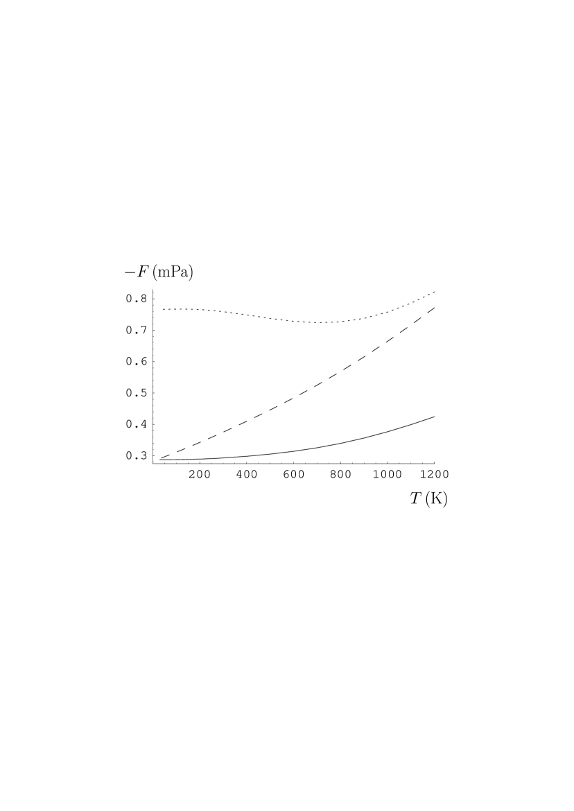
Figure 2: Magnitude of the Casimir force per unit area for dielectrics versus temperature when $a=1\,\mu$m, calculated by the Lifshitz formula. The solid line is for mica, with $\varepsilon=7$. The dotted line is obtained for non-existent non-polar dielectric with $\varepsilon=100$. The dashed line is for polar dielectric with $\varepsilon(0)=100$.

The solid line represents the values calculated in the framework of the impedance approach, and the dashed line is obtained via the Lifshitz formula supplemented by the Drude model with a temperature dependent relaxation parameter [data for $\gamma(T)$ are taken from Ref. 47 ]. It is clearly seen that the dashed line is not monotonous, demonstrating the existence of a wide temperature region where the force modulus decreases with an increase of the temperature (as in Figs. 2, 3 of Ref. 32 ). At the same time, the solid line obtained by using the surface impedance demonstrates the monotonous increase of the magnitude of the Casimir force with temperature in perfect agreement with what is expected from thermodynamics.

It is instructive to know if the nonmonotonous force-temperature relation takes place only for Drude metals or if this may also happen for dielectrics. In Fig. 2, the magnitude of the Casimir force per unit area between dielectrics with $\varepsilon=\mbox{const}$ is shown for different temperatures at a separation of $a=1\,\mu$m. Both solid and dotted lines were obtained from the usual Lifshitz formula (1), (2) with $\varepsilon(i\zeta_{l})=\varepsilon=\mbox{const}$. The solid line is for mica with $\varepsilon=7$; the dotted line coincides with the line in Fig. 5 of Ref. 32 with $\varepsilon=100$. The solid line shows a monotonous increase of the Casimir force with the temperature, as is expected from thermodynamics. On the other hand, the dotted line is not monotonous as the dashed line in Fig. 1. This is, however, artifactual because $\varepsilon$ can be assumed to be independent on the frequency and temperature only in the case of so-called non-polar dielectrics whose atoms or molecules do not have their own dipole moments. The electric susceptibility of non-polar dielectrics arises due to the electronic polarization of atoms and molecules. The values of $\varepsilon$ for non-polar dielectrics are of the order of one 47 ; 48 ; 49 . Large values of $\varepsilon$ can exist only for polar dielectrics where the partial orientation of permanent dipole moments occurs. But for polar dielectrics $\varepsilon$ depends strongly on the frequency and temperature. Specifically, their $\varepsilon$ quickly decreases with the increase of frequency. As a result, at optical and infrared frequencies, which are characteristic for the Casimir effect, the values of $\varepsilon$ are determined by the electronic polarizability 47 and cannot exceed several units. The dielectric permittivity of the polar dielectrics along the imaginary frequency axis can be modeled by 50

$$\varepsilon(i\xi)=1+\sum\limits_{n=1}^{N}\frac{C_{n}}{1+\frac{\xi}{\omega_{n}}},$$ (30)

where the sum describes the effect of possible Debye rotational relaxation frequencies (the absorption spectra of dielectrics are not influential at the characteristic frequencies of the Casimir effect $\omega_{c}$ when the separation between plates is of the order of $1\,\mu$m). In solids, the polarization due to orientation of the permanent dipole moments disappears at rather low frequencies $\sim(10^{7}-10^{8})\,$rad/s 44 . At very high frequencies $\omega>10^{16}\,$rad/s, $\varepsilon$ decreases to unity 40 . Therefore, for the model calculation we may choose $N=2$, $C_{1}=93$, $\omega_{1}=10^{7}$ rad/s, $C_{2}=6$, $\omega_{2}=10^{16}$ rad/s. In this case $\varepsilon(0)=100$ and $\varepsilon\approx 7$ at the characteristic frequency $\omega_{c}$ corresponding to $a=1\,\mu$m.

Eq. (30) was substituted into the Lifshitz formula (1), (2). In Fig. 2, the magnitude of the Casimir force per unit area between the polar dielectrics is represented by the dashed line. It is seen that the force-temperature relation, given by the dashed line, is monotonous as in the case of non-polar dielectrics with small $\varepsilon$, as expected from thermodynamics. From Fig. 2 it is clear that the Casimir force between dielectrics is a monotonous function of the temperature when realistic input data for $\varepsilon$ are substituted into the Lifshitz formula.

In Fig. 3, the Casimir entropy for gold is plotted as a function of the temperature at a separation distance between plates $a=1\,\mu$m. The solid line is drawn in accordance with the impedance approach, i.e. by the use of Eqs. (1), (28) and (29). The dashed line is obtained from the usual Lifshitz formula and Drude model (1)–(3). Evidently, the solid line satisfies all conditions, i.e. positive values of the entropy at nonzero temperatures, and the validity of the Nernst heat theorem. By contrast, the dashed line presents the negative values of the entropy and the violation of the Nernst heat theorem. The analytical proof of the validity of the Nernst heat theorem in the impedance approach can be found in Ref. 36 .

IV Conclusions and discussion

As we have proved above, the substitution of the Drude dielectric function into the Lifshitz formula for the thermal Casimir force leads to the violation of the third law of thermodynamics (the Nernst heat theorem). A rigorous analytical evidence of this statement lies on the fact that at low temperatures the magnitude of the relaxation parameter is much less than the Matsubara frequencies, a property which is always true in the case of perfect crystal lattice. A special analysis of the role of defects or impurities leads to the conclusion that they are incapable to reconcile the calculations of the thermal Casimir force between Drude metals with thermodynamics.

It has been known that the Lifshitz formula combined with the Drude dielectric function predicts a linear (in temperature) large thermal correction to the Casimir force at short separations connected with the second term in the free energy (9) 27 ; 32 ; 33 ; 38 . In recent precision measurement of the Casimir pressure between Au and Cu plates at room temperature 15 ; 16 this correction (which we call “alternative” 16 ) comprises 4.89 mPa and 1.23 mPa at separations $a=300\,$nm and 500 nm, respectively, i.e. 3.6% and 7.24%, respectively, of the total Casimir pressure. For reference, the traditional thermal corrections in the same experimental configuration (computed using the plasma dielectric function 25 ; 26 or the surface impedance 35 ; 36 ) at separations $a=300\,$nm and 500 nm are equal to –0.00863 mPa and –0.00441 mPa, respectively, i.e. only 0.006% and 0.03%, respectively, of the total Casimir pressure (note that the traditional thermal corrections are of the same sign as the Casimir force, i.e. negative). The experimental results of Refs. 15 ; 16 and the extent of their agreement with theory rule out the linear thermal correction to the Casimir force as predicted by the Drude dielectric function substituted into the Lifshitz formula (see Ref. 16 for details). Thus, the combination of the Drude model with the Lifshitz formula is not only thermodynamically inconsistent, but is also in contradiction with experiment.

As we have demonstrated through several computations, the description of real metals based on the surface impedance (Leontovich boundary conditions) is thermodynamically consistent. Unlike the dielectric permittivity, the surface impedance is well defined at all frequencies, even in the domain of the anomalous skin effect. By the use of the Leontovich impedance boundary conditions, instead of the Drude model, the Lifshitz formula is preserved, but the reflection coefficients are expressed in terms of the impedance function. An important point is that different representations for the impedances, which are equivalent for real photons, become nonequivalent in application to the fluctuation fields. As we have shown above, in the case of fluctuating fields the representation (26) for the impedance should be used leading to the Leontovich boundary conditions, whereas the representations (24), (25), when applied to virtual photons, lead to the contradictions with thermodynamics.

In the framework of the impedance approach the value of the zero-frequency term of the Lifshitz formula is prescribed by the form of the impedance and quite satisfactory physical results are obtained. In particular, the Casimir energy and force turn out to be monotonous functions of the temperature, in agreement with what would be expected from thermodynamics. In the region of the infrared optics the results obtained by using the surface impedance coincide with those found earlier through the use of the plasma dielectric function 25 ; 26 . The Casimir entropy in the impedance approach is always positive and vanishes at zero temperature, in accordance with the Nernst heat theorem.

To conclude, we have proved that the Drude dielectric function is not appropriate to describe the thermal Casimir effect in the case of real metals, leading to contradictions with thermodynamics. On the other hand, the Lifshitz formula with the coefficients expressed in terms of the surface impedance is suitable to calculate all the quantities of physical interest.

Figure 1: Magnitude of the Casimir force per unit area for gold versus temperature when $a=1\,\mu$m. The solid line is obtained in the framework of the impedance approach. The dashed line is obtained by using the Drude dielectric function.

Figure 3: Casimir entropy per unit area for two gold semispaces versus temperature, when $a=1\,\mu$m. The solid line is obtained in the framework of the impedance approach. The dashed line is obtained by using the Drude dielectric function.

References

- (1) H. B. G. Casimir, Proc. K. Ned. Akad. Wet. 51, 793 (1948).
- (2) P. W. Milonni, The Quantum Vacuum (Academic Press, San Diego, 1994).
- (3) V. M. Mostepanenko and N. N. Trunov, The Casimir Effect and its Applications (Clarendon Press, Oxford, 1997).
- (4) K. A. Milton, The Casimir Effect (World Scientific, Singapore, 2001).
- (5) M. Kardar and R. Golestanian, Rev. Mod. Phys. 71, 1233 (1999).
- (6) M. Bordag, U. Mohideen, and V. M. Mostepanenko, Phys. Rep. 353, 1 (2001).
- (7) S. K. Lamoreaux, Phys. Rev. Lett. 78, 5 (1997).
- (8) U. Mohideen and A. Roy, Phys. Rev. Lett. 81, 4549 (1998); G. L. Klimchitskaya, A. Roy, U. Mohideen, and V. M. Mostepanenko, Phys. Rev. A 60, 3487 (1999).
- (9) A. Roy and U. Mohideen, Phys. Rev. Lett. 82, 4380 (1999).
- (10) A. Roy, C.-Y. Lin, and U. Mohideen, Phys. Rev. D 60, 111101(R) (1999).
- (11) T. Ederth, Phys. Rev. A 62, 062104 (2000).
- (12) B. W. Harris, F. Chen, and U. Mohideen, Phys. Rev. A 62, 052109 (2000).
- (13) G. Bressi, G. Carugno, R. Onofrio, and G. Ruoso, Phys. Rev. Lett. 88, 041804 (2002).
- (14) F. Chen, U. Mohideen, G. L. Klimchitskaya, and V. M. Mostepanenko, Phys. Rev. Lett. 88, 101801 (2002); Phys. Rev. A 66, 032113 (2002).
- (15) R. S. Decca, D. López, E. Fischbach, and D. E. Krause, Phys. Rev. Lett. 91, 050402 (2003).
- (16) R. S. Decca, E. Fischbach, G. L. Klimchitskaya, D. E. Krause, D. López, and V. M. Mostepanenko, Phys. Rev. D 68, 116003 (2003).
- (17) H. B. Chan, V. A. Aksyuk, R. N. Kleiman, D. J. Bishop, and F. Capasso, Science 291, 1941 (2001); Phys. Rev. Lett. 87, 211801 (2001).
- (18) E. Buks and M. L. Roukes, Phys. Rev. B 63, 033402 (2001).
- (19) M. Bordag, B. Geyer, G. L. Klimchitskaya, and V. M. Mostepanenko, Phys. Rev. D 58, 075003 (1998); 60, 055004 (1999); 62, 011701(R) (2000).
- (20) J. C. Long, H. W. Chan, and J. C. Price, Nucl. Phys. B 539, 23 (1999).
- (21) V. M. Mostepanenko and M. Novello, Phys. Rev. D 63, 115003 (2001).
- (22) E. Fischbach, D. E. Krause, V. M. Mostepanenko, and M. Novello, Phys. Rev. D 64, 075010 (2001).
- (23) G. L. Klimchitskaya and U. Mohideen, Int. J. Mod. Phys. A 17, 4143 (2002).
- (24) E. M. Lifshitz, Sov. Phys. JETP (USA) 2, 73 (1956).
- (25) C. Genet, A. Lambrecht, and S. Reynaud, Phys. Rev. A 62, 012110 (2000); Int. J. Mod. Phys. A 17, 761 (2002).
- (26) M. Bordag, B. Geyer, G. L. Klimchitskaya, and V. M. Mostepanenko, Phys. Rev. Lett. 85, 503 (2000); Phys. Rev. Lett. 87, 259102 (2001).
- (27) M. Boström and B. E. Sernelius, Phys. Rev. Lett. 84, 4757 (2000); Microelectronic Engineering 51–52, 287 (2000); B. E. Sernelius, Phys. Rev. Lett. 87, 139102 (2001); B. E. Sernelius and M. Boström, Phys. Rev. Lett. 87, 259101 (2001).
- (28) V. B. Svetovoy and M. V. Lokhanin, Mod. Phys. Lett. A 15, 1013 (2000); ibid, 1437 (2000); Phys. Lett. A 280, 177 (2001).
- (29) S. K. Lamoreaux, Phys. Rev. Lett. 87, 139101 (2001).
- (30) J. R. Torgerson and S. K. Lamoreaux, quant-ph/0309153.
- (31) I. Brevik, J. B. Aarseth, and J. S. Høye, Phys. Rev. E 66, 026119 (2002).
- (32) J. S. Høye, I. Brevik, J. B. Aarseth, and K. A. Milton, Phys. Rev. E 67, 056116 (2003).
- (33) I. Brevik, J. B. Aarseth, J. S. Høye, and K. A. Milton, quant-ph/0311094.
- (34) G. L. Klimchitskaya and V. M. Mostepanenko, Phys. Rev. A 63, 062108 (2001); G. L. Klimchitskaya, Int. J. Mod. Phys. A 17, 751 (2002).
- (35) B. Geyer, G. L. Klimchitskaya, and V. M. Mostepanenko, Int. J. Mod. Phys. A 16, 3291 (2001); Phys. Rev. A 65, 062109 (2002).
- (36) V. B. Bezerra, G. L. Klimchitskaya, and C. Romero, Phys. Rev. A 65, 012111 (2002).
- (37) B. Geyer, G. L. Klimchitskaya, and V. M. Mostepanenko, Phys. Rev. A 67, 062102 (2003).
- (38) V. B. Svetovoy and M. V. Lokhanin, Phys. Rev. A 67, 022113 (2003).
- (39) V. B. Bezerra, G. L. Klimchitskaya, and V. M. Mostepanenko, Phys. Rev. A 66, 062112 (2002).
- (40) F. Chen, G. L. Klimchitskaya, U. Mohideen, and V. M. Mostepanenko, Phys. Rev. Lett. 90, 160404 (2003).
- (41) C. Kittel, Introduction to Solid State Physics (John Wiley & Sons, Inc., N.Y., 1996).
- (42) N. W. Ashcroft and N. D. Mermin, Solid State Physics (Saunders College Publishing, Philadelphia, 1976).
- (43) L. D. Landau and E. M. Lifshitz, Statistical Physics (Pergamon Press, Oxford, 1958).
- (44) Yu. B. Rumer and M. Sh. Ryvkin, Thermodynamics, Statistical Physics, and Kinetics (Mir Publishers, Moscow, 1980).
- (45) B. E. Sernelius, van der Waals and Casimir forces between metals at finite temperature and the Nernst heat theorem (to appear in Proc. 6th Workshop on QFT under the Influence of External Conditions, Oklahoma, 2003).
- (46) L. D. Landau, E. M. Lifshitz, and L. P. Pitaevskii, Electrodynamics of Continuous Media (Pergamon Press, Oxford, 1984).
- (47) J. A. Stratton, Electromagnetic Theory (McGraw-Hill, New York and London, 1941).
- (48) R. Esquivel, C. Villarreal, and W. L. Mochán, Phys. Rev. A 68, 052103 (2003).
- (49) American Institute of Physics Handbook, ed. D. E. Gray (McGraw-Hill Book Comp., N.Y., 1972).
- (50) C. J. F. Böttcher, Theory of Electric Polarization (Elsevier, New York, 1952).
- (51) H. Frölich, Theory of Dielectrics (Oxford University Press, Oxford, 1949).
- (52) J. Mahanty and B. W. Ninham, Dispersion Forces (Academic Press, London, 1976).