Localization of Two-Dimensional Quantum Walks

Abstract

The Grover walk, which is related to the Grover’s search algorithm on a quantum computer, is one of the typical discrete time quantum walks. However, a localization of the two-dimensional Grover walk starting from a fixed point is striking different from other types of quantum walks. The present paper explains the reason why the walker who moves according to the degree-four Grover’s operator can remain at the starting point with a high probability. It is shown that the key factor for the localization is due to the degeneration of eigenvalues of the time evolution operator. In fact, the global time evolution of the quantum walk on a large lattice is mainly determined by the degree of degeneration. The dependence of the localization on the initial state is also considered by calculating the wave function analytically.

I Introduction

The quantum walks are roughly classified into discrete time quantum walks Y. Aharonov, L. Davidovich, and Zagury (1993); Meyer (1996); Nayak and Vishwanath (2000); A. M. Childs, E. Farhi, and Gutmann (2002); T. A. Brun, H. A. Carteret and Ambainis (2003a, b) and continuous time quantum walks Farhi and Gutmann (1998); D. Aharonov, A. Ambainis, J. Kempe, and Vazirani (2001). We focus on the discrete time quantum walks on a square lattice. The study of the discrete time quantum walks was begun by Aharonov et al. Y. Aharonov, L. Davidovich, and Zagury (1993) in the early 1990s, then it has been investigated by a number of groups. The discrete time quantum walk evolves by repeating simple quantum operations, and it is expected to be realized in a quantum computer. The Grover’s search algorithm Grover (1997), which is one of the most famous quantum algorithms, is especially related to a discrete quantum walk A. M. Childs, R. Cleve, E. Deotto, E. Farhi, S. Gutmann, and Spielman (2002); Childs and Goldstone (2003). Recently Shenvi et al. N. Shenvi, J. Kempe, and BirgittaWhaley (2002) actually proved that a discrete, coined quantum walk can equal Grover’s algorithm. For an introduction of the implementation by a quantum computer, see Travaglione and Milburn Travaglione and Milburn (2002), for example.

The recent concentrated studies make clear mathematical properties of the one-dimensional quantum walks. In particular the one-dimensional Hadamard walk is studied in detail Konno (2002a, b, c); N. Konno, T. Namiki, T. Soshi and Sudbury (2003); M. Bednarska, A. Grudka, P. Kurzyński, T. Luczak, and Wójcik (2003); N. Inui, N. Konishi, N. Konno, and Soshi (2003). In contrast with one-dimensional quantum walks, little about high dimensional quantum walks is known T. D. Mackay, S. D. Bartlett, L. T. Stephanson and Sanders (2002); Moore and Russel (2002); Kempe (2003); B. Tregenna, W. Flanagan, W. Maile, and Kendon (2003); G. Grimmett, S. Janson, and Scudo (2003). Thus the purpose of this study is to investigate a two-dimensional quantum walk called “Grover walk”. A pioneering work for the Grover walk was done by Mackay et al. T. D. Mackay, S. D. Bartlett, L. T. Stephanson and Sanders (2002). Very recently Tregenna et al. B. Tregenna, W. Flanagan, W. Maile, and Kendon (2003) showed numerically that the quantum walker who is controlled by the Grover’s operator is observed at an initial location with a high probability. In this paper, this phenomenon is referred to as “localization”. They showed also that the quantum walker starting from a special initial state spreads out numerically.

The first question we have to ask here is whether the localization remains even after a sufficiently large time. Unfortunately numerical simulations can not give us the exact answer on this problem. Hence it follows that we have to calculate the wave function rigorously. Secondly we ask why the localization is observed only in the Grover walk. There are many different quantum walks, however, the localization is not observed except the Grover walk in our knowledge. Thirdly we would like to know the dependence of the localization on the initial state. We will answer these questions in following sections.

The paper is organized as follows. After defining the Grover walk in section II, we calculate eigenvalues and eigenvectors of the time evolution operator to obtain the wave function in section III. Section IV treats the wave function at the origin and the time-averaged probability. Using the results we show that localization remains even if the system size is infinity. In section V, we concentrate our attention to the localization on an infinite lattice and explain the reason why the Grover walk is special. Furthermore we consider the dependence of the localization on the initial sate and show that the localization disappears at a certain initial state.

II Definition of the two-dimensional quantum walks

II.1 Time evolution of the two-dimensional quantum walks

The Grover walk considered here is a kind of discrete time quantum walks. Thus we begin with defining the two-dimensional quantum walk on the square lattice $Z_{N}=\{(x,y)\in Z^{2}\,|\,-(N-1)/2\leq x\leq(N-1)/2,\,-(N-1)/2\leq y\leq(N-1)/2\}$ with periodic boundary condition. In this paper we assume that the system size $N$ is odd. There are four quantum states at each site:“R”,“L”,“U” and “D” corresponding to right, left, up and down, respectively. The value of wave function for one of these states $S\in\{R,L,U,D\}$ at the position $(x,y)$ and time $t$ is written by $|S,x,y,t\rangle$. The time evolution of $|S,x,y,t\rangle$ is determined as follows:

$$|R,x,y,t+1\rangle=a_{11}|R,x-1,y,t\rangle+a_{12}|L,x-1,y,t\rangle+a_{13}|U,x-1,y,t\rangle+a_{14}|D,x-1,y,t\rangle,$$

$$|L,x,y,t+1\rangle=a_{21}|R,x+1,y,t\rangle+a_{22}|L,x+1,y,t\rangle+a_{23}|U,x+1,y,t\rangle+a_{24}|D,x+1,y,t\rangle,$$

$$|U,x,y,t+1\rangle=a_{31}|R,x,y-1,t\rangle+a_{32}|L,x,y-1,t\rangle+a_{33}|U,x,y-1,t\rangle+a_{34}|D,x,y-1,t\rangle,$$

$$|D,x,y,t+1\rangle=a_{41}|R,x,y+1,t\rangle+a_{42}|L,x,y+1,t\rangle+a_{43}|U,x,y+1,t\rangle+a_{44}|D,x,y+1,t\rangle.\,$$ (1)

This evolution is characterized by the next matrix:

$$A=\left[\begin{array}[]{cccc}a_{11}&a_{12}&a_{13}&a_{14}\\ a_{21}&a_{22}&a_{23}&a_{24}\\ a_{31}&a_{32}&a_{33}&a_{34}\\ a_{41}&a_{42}&a_{43}&a_{44}\end{array}\right].$$ (6)

The matrix corresponding to the Grover walk is defined by

$$A_{0}=\left[\begin{array}[]{rrrr}-\frac{1}{2}&\frac{1}{2}&\frac{1}{2}&\frac{1}{2}\\ \frac{1}{2}&-\frac{1}{2}&\frac{1}{2}&\frac{1}{2}\\ \frac{1}{2}&\frac{1}{2}&-\frac{1}{2}&\frac{1}{2}\\ \frac{1}{2}&\frac{1}{2}&\frac{1}{2}&-\frac{1}{2}\end{array}\right].$$ (11)

We introduce here other two-dimensional quantum walks to compare with the Grover walk by setting following matrices:

$$A_{1} = \left[\begin{array}[]{rrrr}0&0&-\frac{1}{\sqrt{2}}&\hskip 8.53581pt\frac{1}{\sqrt{2}}\\ 0&0&\frac{1}{\sqrt{2}}&\frac{1}{\sqrt{2}}\\ \hskip 5.69054pt\frac{1}{\sqrt{2}}&-\frac{1}{\sqrt{2}}&0&0\\ \frac{1}{\sqrt{2}}&\frac{1}{\sqrt{2}}&0&0\end{array}\right],$$ (16)

$$A_{2} = \left[\begin{array}[]{cccc}-\frac{1}{\sqrt{3}}&0&\frac{1}{\sqrt{3}}&\hskip 5.69054pt\frac{1}{\sqrt{3}}\\ 0&-\frac{1}{\sqrt{3}}&-\frac{1}{\sqrt{3}}&\frac{1}{\sqrt{3}}\\ \frac{1}{\sqrt{3}}&-\frac{1}{\sqrt{3}}&\frac{1}{\sqrt{3}}&0\\ \frac{1}{\sqrt{3}}&\frac{1}{\sqrt{3}}&0&\frac{1}{\sqrt{3}}\end{array}\right].$$ (21)

We define the wave function of the total state at time $t$ by

$$\psi(t) = (\psi_{0,0}(t),\psi_{1,0}(t),\psi_{2,0}(t),\ldots,\psi_{N-1,0}(t),$$ (23)

$$\hskip 8.53581pt\psi_{0,1}(t),\psi_{1,1}(t),\psi_{2,1}(t),\ldots,\psi_{x,y}(t),\ldots,\psi_{N-1,N-1}(t))^{T},$$

where $T$ means the transposed operator and

$$\psi_{x,y}(t)=(|R,x,y,t\rangle,|L,x,y,t\rangle,|U,x,y,t\rangle,|D,x,y,t\rangle)^{T}.$$ (24)

If the initial state $\psi(0)$ is given, then the wave function $\psi(t)$ is calculated by the iteration (1). The iteration can be expressed more compactly by introducing a $4N\times 4N$ unitary matrix $M$ satisfying $\psi(t+1)=M\psi(t)$.

The probability of observing the quantum walker at a given point $(x,y)$ and time $t$ starting from an initial state $\psi(0)$ is defined by

$$P(x,y,t;\psi(0))=\sum_{S\in\{R,L,U,D\}}\langle S,x,y,t|S,x,y,t\rangle.$$ (25)

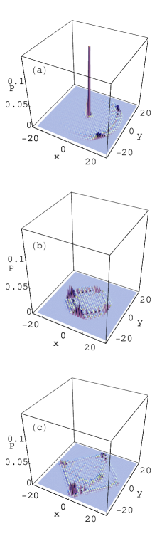
Figure 1: Snapshots of probability distribution $P(x,y,t;\Psi(0))$ at time $t=30$ on a sure lattice with system size $N=51$ with $\Psi(0)=(1,0,\ldots,0)^{T}$. Each of evolutions are determined by the matrices $A_{0}$ (Grover walk), $A_{1}$ and $A_{2}$ defined in (11)-(16) corresponding to (a), (b) and (c). The central peak in (a) shows the localization of the Grover walk.

Fig. 1 shows the probability distribution $P\equiv P(x,y,t;\psi(0))$ corresponding to matrices (a) $A_{0}$ (Grover walk), (b) $A_{1}$ and (c) $A_{2}$ at $t=31$ on the lattice with $N=51$ starting from a pure initial state $\psi(0)=(1,0,\ldots,0)^{T}$. In contrast with (b) and (c) cases, a localization at the origin can be seen only the Grover walk case (a).

III Eignenvalues and eigenvectors of the matrix $M$

III.1 Eigenvalues

To express the wave function as a function of $t$ explicitly we consider the eigenvalues and eigenvectors of the matrix $M$. These are easily obtained by the using the Fourier transform. According to the previous studies D. Aharonov, A. Ambainis, J. Kempe, and Vazirani (2001), the eigenvaleus of the matrix $M$ are given by a set of eigenvalues of the following matrix

$$H_{n,m}(A)=\left[\begin{array}[]{cccc}\omega^{-n}&0&0&0\\ 0&\omega^{n}&0&0\\ 0&0&\omega^{-m}&0\\ 0&0&0&\omega^{m}\end{array}\right]\left[\begin{array}[]{cccc}a_{11}&a_{12}&a_{13}&a_{14}\\ a_{21}&a_{22}&a_{23}&a_{24}\\ a_{31}&a_{32}&a_{33}&a_{34}\\ a_{41}&a_{42}&a_{43}&a_{44}\end{array}\right],$$ (34)

where $\omega=e^{2\pi i/N}$. The integers $n$ and $m$ are quantum numbers in a wave number space and they take values between 0 and $N-1$. Since there are four components in $H_{n,m,}(A)$, the number of eigenvalues is $(4N)^{2}$, if not consider the degeneration of eigenvalues, and each eigenvalue is labeled by $n,m\in\{0,1,\ldots,N-1\}$ and $k\in\{1,2,3,4\}$. As a result, when $n\neq m$, the eigenvalues of the matrix $M$ corresponding to the Grover walker, $\lambda_{n,m,k}$, are given by

$$\lambda_{n,m,1} = -1,$$ (35)

$$\lambda_{n,m,2} = 1,$$ (36)

$$\lambda_{n,m,3} = \frac{-\cos\xi_{m}-\cos\xi_{n}-{\sqrt{-4+{\left(\cos\xi_{m}+\cos\xi_{n}\right)}^{2}}}}{2},$$ (37)

$$\lambda_{n,m,4} = \frac{-\cos\xi_{m}-\cos\xi_{n}+{\sqrt{-4+{\left(\cos\xi_{m}+\cos\xi_{n}\right)}^{2}}}}{2},$$ (38)

where $\xi_{j}=2j\pi/N$. When $n=m$, the eigenvalues are written as

$$\lambda_{n,n,1} = -1,$$ (39)

$$\lambda_{n,n,2} = 1,$$ (40)

$$\lambda_{n,n,3} = -\omega^{n},$$ (41)

$$\lambda_{n,n,4} = -\omega^{-n}.$$ (42)

III.2 Eigenvectors

We write the eigenvectors corresponding to the eigenvalues $\lambda_{n,m,k}$ as $\phi_{n,m,k}$ and we let $\phi_{i,n,m,k}$ be $i$-th element of $\phi_{n,m,k}$. If $-(N-1)/2\leq x,y\leq(N-1)/2$ and $1\leq j\leq 4$, we find integers $x,y$ and $j$ satisfying an equation $4Ny+4x+j+2N^{2}-2=i$ for a given natural number $i$. Using these $x,y$ and $j$, the $i$-th element of $\phi_{n,m,k}$, which generates an orthonormal basis is given by

$$\phi_{i,n,m,k} = \frac{v_{j,n,m,k}\omega^{nx+my}}{N\sqrt{\sum_{j=1}^{4}|v_{j,n,m,k}|^{2}}},$$ (43)

where $v_{j,n,m,k}$ is the $j$-th element of the eigenvector of $H_{n,m,k}$. We show a set of eigenvectors of $v_{n,m,k}\equiv(v_{1,n,m,k},\cdots,v_{4,n,m,k})^{T}$ in the following:

Case 1: $m=0,n>0,k=1$

$$v_{n,0,1}=\left[\begin{array}[]{c}1\\ -1\\ 0\\ 0\end{array}\right],$$ (48)

Case 2: $m=0,n>0$ and $k>1$

$$v_{n,0,k}=\left[\begin{array}[]{c}\lambda_{n,0,k}+\beta_{n}\\ \lambda_{n,0,k}+\beta_{n}\\ \beta_{n}\lambda_{n,0,k}+\beta_{n}\\ 2\lambda_{n,0,k}^{2}+\beta_{n}\lambda_{n,0,k}-\beta_{n}\end{array}\right],$$ (53)

Case 3: $n=m$

$$\{v_{n,n,k}|1\leq k\leq 4\}=\left\{\left[\begin{array}[]{c}-\alpha_{n}\\ 1\\ -\alpha_{n}\\ 1\end{array}\right],\hskip 14.22636pt\left[\begin{array}[]{c}\alpha_{n}\\ 1\\ \alpha_{n}\\ 1\end{array}\right],\hskip 14.22636pt\left[\begin{array}[]{c}0\\ -1\\ 0\\ 1\end{array}\right],\hskip 14.22636pt\left[\begin{array}[]{c}-1\\ 0\\ 1\\ 0\end{array}\right]\right\},$$ (70)

Case 4: $n+m=N$

$$\{v_{n,N-n,k}|1\leq k\leq 4\}=\left\{\left[\begin{array}[]{c}1\\ -1/\alpha_{n}\\ -1/\alpha_{n}\\ 1\end{array}\right],\hskip 14.22636pt\left[\begin{array}[]{c}1\\ 1/\alpha_{n}\\ 1/\alpha_{n}\\ 1\end{array}\right],\hskip 14.22636pt\left[\begin{array}[]{c}0\\ -1\\ 1\\ 0\end{array}\right],\hskip 14.22636pt\left[\begin{array}[]{c}-1\\ 0\\ 0\\ 1\end{array}\right]\right\},$$ (87)

Case 5: otherwise

$$v_{n,m,k}=\left[\begin{array}[]{c}\alpha_{n}^{2}\lambda^{2}_{n,m,k}+(\alpha_{n}+\alpha_{n}^{2}\beta_{m})\lambda_{n,m,k}+\alpha_{n}\beta_{m}\\ \lambda_{n,m,k}^{2}+(\alpha_{n}+\beta_{m})\lambda_{n,m,k}+\alpha_{n}\beta_{m}\\ \alpha_{n}\beta_{m}\lambda_{n,m,k}^{2}+(\beta_{m}+\alpha_{n}^{2}\beta_{m})\lambda_{n,m,k}+\alpha_{n}\beta_{m}\\ 2\alpha_{n}\lambda_{n,m,k}^{3}+(1+\alpha_{n}^{2}+\alpha_{n}\beta_{m})\lambda_{n,m,k}^{2}-\alpha_{n}\beta_{m}\end{array}\right],$$ (92)

where $\alpha_{n}=\omega^{-n}$ and $\beta_{m}=\omega^{-m}$.

IV Wave function of the Grover walk

IV.1 Expansion of wave function in terms of eigenvalues

Since we have obtained the complete eigenvalues and normalized orthogonal eigenvectors, we can express the wave function as a function of time. Before we present the wave function, we number the states R, L, U, and D from 1 to 4, respectively. Let $l(S)$ be the number of the state “S”. Then we have the wave function $|S,x,y,t\rangle$:

$$|S,x,y,t\rangle = \sum_{j=1}^{4N^{2}}\sum_{n=0}^{N-1}\sum_{m=0}^{N-1}\sum_{k=1}^{4}\phi_{i,n,m,k}\phi_{j,n,m,k}^{\ast}\psi_{j}(0)\lambda_{n,m,k}^{t},$$ (93)

where $i=4Ny+4x+l(S)+2N^{2}-2$ and $\psi_{j}(0)$ is the $j$-th element of the initial vector $\psi(0)$.

As shown in (38), the eigenvalues degenerate strongly. Thus we try to expand the wave function by distinct eigenvalues. The eigenvalue $\lambda_{n,m,1}=-1$ always exists for any combination $n$ and $m$. Furthermore the $\lambda_{n,m,3}$ and $\lambda_{n,m,4}$ become $-1$ for $n=m=0$. If $n>0$ and $m>0$, then the eigenvalues $\lambda_{n,m,k}$ are distinct for fixed $n$ and $m$. Therefore the condition $\lambda_{n,m,k}=\lambda_{n^{\prime},m^{\prime},k}$ is equivalent to the following condition

$$\cos\xi_{m}+\cos\xi_{n}=\cos\xi_{m^{\prime}}+\cos\xi_{n^{\prime}}.$$ (94)

A set of a pair $(n^{\prime},m^{\prime})$ belonging to the same eigenvalue $\lambda_{n,m,k}$ for $k>2$ and $n>0$ is given by

$$\Omega(n,m)=\left\{\begin{array}[]{l}\{(n,0),(0,n),(N-n,0),(0,N-n)\}\hskip 8.53581pt\mbox{for}\hskip 8.53581ptm=0,\\ \{(n,n),(n,N-n)\}\hskip 8.53581pt\mbox{for}\hskip 8.53581ptn=m,\\ \{(n,m),(n,N-m),(N-n,m),(N-n,N-m),\\ \,\,(m,n),(m,N-n),(N-m,n),(N-m,N-n)\}\hskip 8.53581pt\mbox{otherwise}.\end{array}\right.$$ (98)

To express the wave function compactly using the set $\Omega(n,m)$ we define the following functions:

$$c_{i,j,0,0,k} = \frac{v_{i,0,0,k}v_{j,0,0,k}^{\ast}\psi_{j}(0)}{\sqrt{\sum_{i=1}^{4}|v_{i,0,0,k}|^{2}}\sqrt{\sum_{j=1}^{4}|v_{j,0,0,k}|^{2}}},$$ (99)

$$c_{i,j,n,m,k} = \sum_{n^{\prime},m^{\prime}\in\Omega(n,m)}\frac{v_{i,n^{\prime},m^{\prime},k}v_{j,n^{\prime},m^{\prime},k}^{\ast}\psi_{j}(0)}{\sqrt{\sum_{i=1}^{4}|v_{i,n^{\prime},m^{\prime},k}|^{2}}\sqrt{\sum_{j=1}^{4}|v_{j^{\prime},n^{\prime},m^{\prime},k}|^{2}}}$$ (100)

$$\hskip 170.71652pt\mbox{for}\hskip 5.69054ptn>0\hskip 5.69054pt\mbox{and}\hskip 5.69054ptm>0.$$

We note here the reason why the system size is restricted to odd in this paper. In the case of odd, the degree of degeneration of eigenvalues is eight at the most except for the eigenvalues $-1$ and $1$. On the other, the eigenvalues with large degree of degeneration exist in addition to the $1$ and $-1$ in the case of even. This fact does not lead us to fatal difficulty, but the calculation becomes more complicated than that in the odd case.

We now have another expression of wave function:

$$|S,x,y,t\rangle = \frac{1}{N^{2}}\sum_{j=1}^{4N^{2}}\left[C_{i,j,1}+C_{i,j,-1}(-1)^{t}+\sum_{n=1}^{\frac{N-1}{2}}\sum_{k=3}^{4}c_{i,j,n,0,k}\lambda_{n,0,k}^{t}\right.$$ (101)

$$\hskip 42.67912pt+\left.\sum_{n=1}^{N-1}\sum_{k=3}^{4}c_{i,j,n,n,k}\lambda_{n,n,k}^{t}+\sum_{n=1}^{\frac{N-3}{2}}\sum_{m=n+1}^{\frac{N-1}{2}}\sum_{k=3}^{4}c_{i,j,n,m,k}\lambda_{n,m,k}^{t}\right],$$

where

$$C_{i,j,1} = c_{i,j,0,0,2}+\sum_{n=1}^{\frac{N-1}{2}}c_{i,j,n,0,2}+\sum_{n=1}^{N-1}c_{i,j,n,n,2}+\sum_{n=1}^{\frac{N-3}{2}}\sum_{m=n+1}^{\frac{N-1}{2}}c_{i,j,n,m,2},$$ (102)

$$C_{i,j,-1} = c_{i,j,0,0,1}+c_{i,j,0,0,3}+c_{i,j,0,0,4}+\sum_{n=1}^{\frac{N-1}{2}}c_{i,j,n,0,1}+\sum_{n=1}^{N-1}c_{i,j,n,n,1}+\sum_{n=1}^{\frac{N-3}{2}}\sum_{m=n+1}^{\frac{N-1}{2}}c_{i,j,n,m,1}.$$ (103)

and $i=4Ny+4x+l(S)+2N^{2}-2$. In the formula (101), $C_{i,j,1}$ and $C_{i,j,-1}(-1)^{t}$ give the contribution of the eigenvalue $1$ and $-1$ to the wave function. The remaining terms are corresponding to the eigenvalues for $k=3$ and 4.

We move on more specific cases. In order to show the localization we calculate $|R,0,0,t\rangle$ for the Grover walk starting from a pure state $|R,0,0,0\rangle=1$. We refer this special initial state as $\phi_{R}$. The values in (99), (100) and (102), (103) can be obtained after some algebra by

$$C_{1,1,1}=\frac{N^{2}}{4},\hskip 8.53581ptC_{i,1,-1}=\frac{1}{2}+\frac{N^{2}}{4},$$ (104)

$$c_{1,1,n,0,k}=1,\hskip 8.53581pt\mbox{for}\hskip 8.53581pt\forall k,$$ (105)

$$c_{1,1,n,n,1}=c_{1,1,n,n,2}=\frac{1}{2},\hskip 5.69054ptc_{1,1,n,n,3}=0,\hskip 5.69054ptc_{1,0,n,n,4}=1,$$ (106)

$$c_{1,1,n,m,k}=2,\hskip 8.53581pt\mbox{for}\hskip 8.53581pt\forall k.$$ (107)

V Time-averaged probability

V.1 Definition of time-averaged probability

We begin with considering the probability $P(S,t;\phi_{0},N)$ that a walker in the state “S” at the origin on a square lattice with size $N$ starting form an initial state $\phi_{0}$. The probability $P(S,t;\phi_{0},N)$ is calculated from the relation

$$P(S,t;\phi_{0},N)\equiv\langle S,0,0,t|S,0,0,t\rangle.$$ (108)

The probability $P(S,t;\phi_{0},N)$ dose not converge to a fixed value in the limit $t\rightarrow\infty$ in contrast with classical random walks. Thus we introduce time-averaged probability $\bar{P}(S;\phi_{0},N)$ defined by

$$\bar{P}(S;\phi_{0},N)\equiv\lim_{T\rightarrow\infty}\frac{1}{T}\sum_{t=0}^{T-1}P(S,t;\phi_{0},N).$$ (109)

Let us calculate $\bar{P}(S;\phi_{R},N)$, which is the time-averaged probability starting a pure state $\phi_{R}$. Submitting the wave function with coefficients (104)-(107) into the definition (108), we find the cross terms in the form $\lambda_{n,m,k}\lambda_{n^{\prime},m^{\prime},k^{\prime}}$. If the eigenvalue $\lambda_{n,m,k}$ is different from $\lambda_{n^{\prime},m^{\prime},k^{\prime}}$, the time-averaged value $\lim_{T\rightarrow\infty}\sum_{t=0}^{T-1}(\lambda_{n,m,k})^{t}(\lambda_{n^{\prime},m^{\prime},k^{\prime}}^{\ast})^{t}/T$ vanishes. Thus we have

$$\bar{P}(S;\phi_{0},N) = \frac{1}{N^{4}}\left[\left|\sum_{j=1}^{4N^{2}}C_{i,j,1}\right|^{2}+\left|\sum_{j=1}^{4N^{2}}C_{i,j,-1}\right|^{2}+\sum_{n=1}^{\frac{N-1}{2}}\sum_{k=3}^{4}\left|\sum_{j=1}^{4N^{2}}c_{i,j,n,0,k}\right|^{2}\right.$$ (110)

$$\left.+\sum_{n=1}^{N-1}\sum_{k=3}^{4}\left|\sum_{j=1}^{4N^{2}}c_{i,j,n,n,k}\right|^{2}+\sum_{n=1}^{\frac{N-3}{2}}\sum_{m=n+1}^{\frac{N-1}{2}}\sum_{k=3}^{4}\left|\sum_{j=1}^{4N^{2}}c_{i,j,n,m,k}\right|^{2}\right].$$

Plugging equations (104)-(107) into (110), the time-averaged probability $\bar{P}(R;\phi_{R},N)$ is given by

$$\bar{P}(R;\phi_{R},N)=\frac{1}{8}+\frac{5}{4N^{2}}-\frac{2}{N^{3}}+\frac{5}{4N^{4}}.$$ (111)

The time-averaged probability $\bar{P}(S;\phi_{R},N)$ is a monotone decreasing function in $N$ and it converges to 1/8 in the limit $N\rightarrow\infty$. Thus $\bar{P}(S;\phi_{R},N)$ is larger than 1/8 for any odd $N$. It means that the quantum walker centralizes at the origin.

We must pay attention to the dependence of the wave function on the parity of time. The value of wave function at odd time is small in comparison with the value at even time. It is similar to the fact that the probability of return to the origin at odd time is zero in a classical random walk on an infinite square lattice. Let $\bar{P}_{e}(S;\phi_{R},N)$ and $\bar{P}_{o}(S;\phi_{R},N)$ be the time-averaged probabilities over even time and odd time, respectively. Then we have

$$\bar{P}_{e}(R;\phi_{R},N) = \frac{1}{4}+\frac{3}{2N^{2}}-\frac{2}{N^{3}}+\frac{5}{4N^{4}},$$ (112)

$$\bar{P}_{o}(R;\phi_{R},N) = \frac{1}{N^{2}}-\frac{2}{N^{3}}+\frac{5}{4N^{4}}.$$ (113)

The probability averaged over odd time $\bar{P}_{o}(R;\phi_{R},N)$ converges zero in the limit $N\rightarrow\infty$. Thus there is a relation $\bar{P}_{e}(R;\phi_{R},N)=2\bar{P}(R;\phi_{R},N)$ in the limit $N\rightarrow\infty$.

V.2 The time-averaged probability in the limit $N\rightarrow\infty$

We now proceed to the probability $P(S,t;\phi_{R},N)$ in the limit $N\rightarrow\infty$. The only first and second terms in (110) remain in the limit of $N\rightarrow\infty$. Thus its calculation becomes easy as shown below:

$$\bar{P}_{\infty}(S;\phi_{R}) \equiv \lim_{N\rightarrow\infty}\bar{P}(S;\phi_{R},N),$$ (114)

$$= \lim_{N\rightarrow\infty}\frac{1}{N^{4}}\left(\left|C_{i,0,1}\right|^{2}+\left|C_{i,0,-1}\right|^{2}\right).$$ (115)

Furthermore the constant and the single summation in $C_{i,j,1}$ and $C_{i,j,-1}$ do not contribute to $\bar{P}_{\infty}(S;\phi_{R})$. Consequently, the probability $\bar{P}_{\infty}(S;\phi_{R})$ is given by

$$\bar{P}_{\infty}(S;\phi_{R})=\left(\lim_{N\rightarrow\infty}\frac{1}{N^{2}}\sum_{n=1}^{\frac{N-3}{2}}\sum_{m=n+1}^{\frac{N-1}{2}}c_{i,0,n,m,1}\right)^{2}+\left(\lim_{N\rightarrow\infty}\frac{1}{N^{2}}\sum_{n=1}^{\frac{N-3}{2}}\sum_{m=n+1}^{\frac{N-1}{2}}c_{i,0,n,m,2}\right)^{2}.$$ (116)

Let consider time-averaged probabilities in $N\rightarrow\infty$ for all possible states at the origin. The value of $c_{i,0,n,m,1}$ and $c_{i,0,n,m,2}$ as function $n$ and $m$ are given by

$$c_{2,0,n,m,1} = \frac{2\,\left(\cos\xi_{m}+\cos\xi_{n}-2\,\cos\xi_{m}\,\cos\xi_{n}\right)}{-2+\cos\xi_{m}+\cos\xi_{n}},$$ (117)

$$c_{2,0,n,m,2} = \frac{2\,\left(\cos\xi_{m}+\cos\xi_{n}+2\,\cos\xi_{m}\,\cos\xi_{n}\right)}{2+\cos\xi_{m}+\cos\xi_{n}},$$ (118)

$$c_{i,0,n,m,1} = \frac{8\sin^{2}(\xi_{m}/2)\sin^{2}(\xi_{n}/2)}{2-\cos\xi_{m}-\cos\xi_{n}}\hskip 8.53581pt\mbox{for}\hskip 8.53581pti=3,4,$$ (119)

$$c_{i,0,n,m,2} = \frac{8\cos^{2}(\xi_{m}/2)\cos^{2}(\xi_{n}/2)}{2+\cos\xi_{m}+\cos\xi_{n}}\hskip 8.53581pt\mbox{for}\hskip 8.53581pti=3,4.$$ (120)

The double summations in (116) in the limit $N\rightarrow\infty$ are calculated by replacing the summations into the following integrals:

$$\lim_{N\rightarrow\infty}\frac{1}{N^{2}}\sum_{n=1}^{\frac{N-3}{2}}\sum_{m=n+1}^{\frac{N-1}{2}}c_{2,0,n,m,1} = \frac{1}{8\pi^{2}}\int_{0}^{\pi}dx\int_{0}^{\pi}dy\frac{2\,\left(\cos x+\cos y-2\,\cos x\,\cos y\right)}{-2+\cos x+\cos y},$$ (121)

$$= \frac{1}{4}-\frac{1}{\pi},$$

$$\lim_{N\rightarrow\infty}\frac{1}{N^{2}}\sum_{n=1}^{\frac{N-3}{2}}\sum_{m=n+1}^{\frac{N-1}{2}}c_{3,0,n,m,1} = \frac{1}{2\pi^{2}}\int_{0}^{\frac{\pi}{2}}dx\int_{0}^{\frac{\pi}{2}}dy\frac{8\sin^{2}x\sin^{2}y}{2-\cos 2x-\cos 2y},$$ (122)

$$= \frac{1}{4}-\frac{1}{2\pi}.$$

Similarly we can calculate the summation for $c_{2,0,n,m,2}$ and $c_{3,0,n,m,2}$, and we have the same values $1/4-1/\pi$ and $1/4-1/2\pi$. Finally the time-averaged probabilities are given by

$$\bar{P}_{\infty}(R;\phi_{R}) = \frac{1}{8},$$ (123)

$$\bar{P}_{\infty}(L;\phi_{R}) = \frac{1}{8}+\frac{2}{\pi^{2}}-\frac{1}{\pi},$$ (124)

$$\bar{P}_{\infty}(U;\phi_{R}) = \frac{1}{8}+\frac{1}{2\pi^{2}}-\frac{1}{2\pi},$$ (125)

$$\bar{P}_{\infty}(D;\phi_{R}) = \frac{1}{8}+\frac{1}{2\pi^{2}}-\frac{1}{2\pi}.$$ (126)

Summing $\bar{P}_{\infty}(S;\phi_{R})$ over all possible states, the time-averaged probability that a quantum walker exists at the origin is

$$\bar{P}_{\infty}(\phi_{R}) = \bar{P}_{\infty}(R;\phi_{R})+\bar{P}_{\infty}(L;\phi_{R})+\bar{P}_{\infty}(U;\phi_{R})+\bar{P}_{\infty}(D;\phi_{R}),$$ (127)

$$= \frac{1}{2}+\frac{3}{\pi^{2}}-\frac{2}{\pi}$$

V.3 Dependence of the time-averaged probability on an initial state

If the Grover walk starts from the pure state, then the localization of the quantum walker at the origin was shown in the previous section. The numerical results obtained by Tregenna et al. B. Tregenna, W. Flanagan, W. Maile, and Kendon (2003), however, suggests that the time-averaged probability at origin of the Grover walk with a certain mixed initial state becomes zero. To confirm this observation we consider the wave function at the origin starting the next mixed initial state

$$\phi(\alpha,\beta)=\alpha|R,0,0,0\rangle+\beta|L,0,0,0\rangle,$$ (128)

where $|\alpha|^{2}+|\beta|^{2}=1$. In the formula in (101) the coefficients corresponding to $j>2$ are zero and the coefficients corresponding to $j=1$ are already computed in (107). Thus we consider the only coefficients corresponding to $j=2$. Suppose that $\psi(0)=\phi_{L}=(0,1,0,\ldots,0)^{T}$. Then we obtain

$$C_{1,2,1} = -\frac{7}{4}+\frac{3N}{2}-\sum_{n=1}^{\frac{N-1}{2}}\frac{8}{3+\cos\xi_{n}}$$ (129)

$$\hskip 28.45274pt+\sum_{n=1}^{\frac{N-3}{2}}\sum_{m=n+1}^{\frac{N-1}{2}}\frac{2\,\left(\cos\xi_{m}+\cos\xi_{n}+2\,\cos\xi_{m}\,\cos\xi_{n}\right)}{2+\cos\xi_{m}+\cos\xi_{n}},$$

$$C_{1,2,-1} = \frac{3}{4}-\frac{N}{2}+\sum_{n=1}^{\frac{N-3}{2}}\sum_{m=n+1}^{\frac{N-1}{2}}\frac{2\,\left(\cos\xi_{m}+\cos\xi_{n}-2\,\cos\xi_{m}\,\cos\xi_{n}\right)}{-2+\cos\xi_{m}+\cos\xi_{n}},$$ (130)

$$c_{1,2,n,0,3} = c_{1,2,n,0,4}=-1+\frac{4}{3+\cos{\xi_{n}}},$$ (131)

$$c_{1,2,n,n,3} = c_{1,2,n,n,4}=0,$$ (132)

$$c_{1,2,n,m,3} = c_{1,2,n,m,4}=\frac{4(\cos\xi_{m}-\cos\xi_{n})^{2}}{6-\cos(2\xi_{m})-\cos(2\xi_{n})-4\cos\xi_{n}\cos\xi_{m}}\hskip 8.53581pt\mbox{for}\hskip 8.53581ptm>n.$$ (133)

We now can calculate the time-averaged probability $\bar{P}(R;\phi(\alpha,\beta),N)$ for any odd system size $N$ by combining (104) - (107) with (129) - (133). However it is rather complicated. Thus we show only the result in the limit of $N\rightarrow\infty$. The time-averaged probability $\bar{P}_{\infty}(R;\phi(\alpha,\beta))$ is obtained by replacing the summations to the integrals in the same way described in the previous section, and it becomes

$$\bar{P}_{\infty}(R;\phi(\alpha,\beta))=\frac{1}{8}\left|\alpha+\left(1-\frac{4}{\pi}\right)\beta\right|^{2}.$$ (134)

Similarly we have the time-averaged probability corresponding to the “L” state

$$\bar{P}_{\infty}(L;\phi(\alpha,\beta))=\frac{1}{8}\left|\beta+\left(1-\frac{4}{\pi}\right)\alpha\right|^{2}.$$ (135)

Fig. 2 shows $\bar{P}_{R}(\alpha)\equiv\bar{P}_{\infty}(R;\phi(\alpha,\sqrt{1-\alpha^{2}}))$ and $\bar{P}_{L}(\alpha)\equiv\bar{P}_{\infty}(L;\phi(\alpha,\sqrt{1-\alpha^{2}}))$ for $\alpha\in[-1,1]$. The time-averaged probability $\bar{P}_{R}(\alpha)$ becomes zero at $\alpha_{min}$ given by

$$\alpha_{min} = \sqrt{1-\frac{\pi^{2}}{16-8\pi+2\pi^{2}}},$$ (136)

and it takes the maximum value at $\alpha_{max}$ given by

$$\alpha_{max} = \frac{\pi}{\sqrt{16-8\pi+2\pi^{2}}}.$$ (137)

Since the value $\alpha=1$ and $\alpha=-1$ indicate the pure state, it is found that the time-averaged probability $\bar{P}_{R}(\alpha)$ takes the maximum at the mixed initial state. As shown in the numerical calculation B. Tregenna, W. Flanagan, W. Maile, and Kendon (2003), the quantum walk starting from a certain initial state spreads out. Although the time-averaged probability $\bar{P}_{R}(\alpha)$ becomes zero at $\alpha=\alpha_{min}$, the quantum walker remains at the origin. Put another way, the component of the time-averaged probability corresponding to the “R” state converges to zero, but other component remains positive. Therefore we can say that the quantum walker in the state “R” perfectly converts into other state in the limit $t\rightarrow\infty$ at $\alpha=\alpha_{min}$.

Let us consider the time-averaged probability for more general initial states defined by

$$\phi(\alpha,\beta,\gamma,\zeta)=\alpha|R,0,0,0\rangle+\beta|L,0,0,0\rangle+\gamma|U,0,0,0\rangle+\zeta|D,0,0,0\rangle,$$ (138)

where $|\alpha|^{2}+|\beta|^{2}+|\gamma|^{2}+|\zeta|^{2}=1$. Repeating the procedure described above yields the time-averaged probability for this initial state:

$$\bar{P}_{\infty}(R;\phi(\alpha,\beta,\gamma,\zeta))=\left|\frac{\alpha}{2\,{\sqrt{2}}}-{\sqrt{\frac{1}{8}+\frac{2}{{\pi}^{2}}-\frac{1}{\pi}}}\beta\ +{\sqrt{\frac{1}{8}+\frac{1}{2\,{\pi}^{2}}-\frac{1}{2\,\pi}}}\,(\gamma+\zeta)\right|^{2}.$$ (139)

Taking symmetry into account, the other components are given by

$$\bar{P}_{\infty}(L;\phi(\alpha,\beta,\gamma,\zeta)) = \bar{P}_{\infty}(R;\phi(\beta,\alpha,\gamma,\zeta)),$$ (140)

$$\bar{P}_{\infty}(U;\phi(\alpha,\beta,\gamma,\zeta)) = \bar{P}_{\infty}(R;\phi(\gamma,\zeta,\alpha,\beta)),$$ (141)

$$\bar{P}_{\infty}(D;\phi(\alpha,\beta,\gamma,\zeta)) = \bar{P}_{\infty}(R;\phi(\zeta,\gamma,\alpha,\beta)).$$ (142)

The condition for which all components in (139) - (142) become zero is obtained by

$$\alpha=e^{i\theta}/2,\hskip 8.53581pt\beta=\alpha,\hskip 8.53581pt\gamma=-\alpha,\hskip 8.53581pt\zeta=-\alpha.$$ (143)

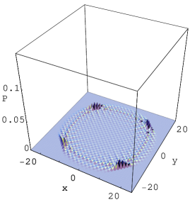
Figure 3: The probability $P(x,y,t;\Psi(0))$ of Grover walk at $t=30$ starting a mixed state $\Psi(0)=(e^{i/3},e^{i/3},-e^{i/3},-e^{i/3},0,\ldots,0)^{T}$ with $N=51$. The central localization in Fig. 1 (a) disappears.

Setting $\theta=0$, we confirm the numerical results given by Tregenna et al. B. Tregenna, W. Flanagan, W. Maile, and Kendon (2003), which claim that the probability of $\bar{P}_{\infty}(S;\phi(\alpha,\beta,\gamma,\zeta))$ becomes zero for any state $S$ by setting $\alpha=\beta=-\gamma=-\zeta=1/2$. Fig. 3 shows a snapshot after $30$ steps on a square lattice with $N=51$ starting from an initial state with $\theta=1/3$ in (143). One definitely finds that the localization disappears. On the other hand, the summation of $\bar{P}_{\infty}(S;\phi(\alpha,\beta,\gamma,\zeta))$ over all possible states takes a maximum values $2+8/\pi^{2}-8/\pi$=0.26409.. at $\alpha=\beta=\gamma=\zeta=1/2$. Thus the time-averaged probability over even time is larger than 1/2.

V.4 Conditions of the localization

We saw that a spike exists at the origin in Grover walk, but the two-dimensional quantum walkers governed by the matrix $A_{1}$ and $A_{2}$ spread out. The significant difference between the Grover walk and other quantum walks is the degree of eigenvalues. For example, the eigenvalues of $H_{n,m}$ with $A_{1}$ are given by

$$\left[\begin{array}[]{r}\lambda_{n,m,1}\\ \lambda_{n,m,2}\\ \lambda_{n,m,3}\\ \lambda_{n,m,4}\end{array}\right]=\left[\begin{array}[]{r}\sqrt{i\cos\xi_{n}\cos\xi_{m}+f_{n,m}},\\ -\sqrt{i\cos\xi_{n}\cos\xi_{m}+f_{n,m}},\\ \sqrt{i\cos\xi_{n}\cos\xi_{m}-f_{n,m}},\\ -\sqrt{i\cos\xi_{n}\cos\xi_{m}-f_{n,m}},\\ \end{array}\right],$$ (152)

where

$$f_{n,m}=\sqrt{\sin^{2}\xi_{m}+\cos^{2}\xi_{n}\cos^{2}\xi_{m}}.$$ (153)

We find no common eigenvalues to all value $n$ and $m$ such as $-1$ and $1$ in $\lambda_{n,m,k}$. If a quantum walker exists only at the origin initially, the coefficient $c_{i,j,n,m,k}$ in (110) takes non-zero value for only one $j$. Therefore the summation over $j$ in (110) does not depend on the system size and the summation over $n$ and $k$ increases with the system size. Accordingly, the order of third and fourth term in (110) is $\cal O\mit(N^{-3})$. Similarly the order of the fifth term in (110) is $\cal O\mit(N^{-2})$. As a result, these terms vanish in the limit $N\rightarrow\infty$. As shown in (102) and (103), since $C_{i,j,1}$ and $C_{i,j,-1}$ contain double summations, the order of them is $\cal O\mit(N^{2})$. This large contribution to the time-averaged probability comes from the fact that the eigenvalues $-1$ and $1$ exist for any $n$ and $m$ in common. From the above consideration one conjectures that there is another two-dimensional quantum walk in which the walker centralize at the origin. Thus we find a new matrix $A_{4}$ such that $H_{n,m}(A_{4})$ contains eigenvalue $-1$ and $1$ independently on the value $n$ and $m$. Suppose that the matrix $A_{4}$ is real symmetric matrix. Then a possible matrix is given by

$$A_{4}=\left[\begin{array}[]{cccc}-p&q&\sqrt{pq}&\sqrt{pq}\\ q&-p&\sqrt{pq}&\sqrt{pq}\\ \sqrt{pq}&\sqrt{pq}&-q&p\\ \sqrt{pq}&\sqrt{pq}&p&-q\end{array}\right],$$ (158)

where $q=1-p$. The Grover walk is corresponding to $p=1/2$. As an example we show the probability $P(x,y,t;\phi_{R})$ of a quantum walk which is characterized by the matrix $A_{4}$ with $p=1/3$ and $q=2/3$ in Fig.4. We clearly recognize the existence of a spike at the origin.

VI Summary

We have shown analytically that the localization of the Grover walk at the initial position can be surely measured for any odd system size. On the other hand, we have also shown that we can chose special initial states with which the quantum walk disappears at the initial position in $N\rightarrow\infty$. As pointed out by Tregenna et al. B. Tregenna, W. Flanagan, W. Maile, and Kendon (2003), this different behavior can be used to control the Grover’s search. We here summarize the reason why the localization exists in the Grover walk starting from a local position.

There are $16N^{2}$ quantum states in the Grover walk on the square lattice including $N^{2}$ sites. Therefore the number of eigenvalues and eigenvectors of the time-evolution operator is also $16N^{2}$. Since the wave function at time $t$ is expressed by a liner combination of the $t$-th power of the eigenvalue in which the coefficients are given by the product of component of eigenvectors. Each component of the eigenvector decrease in inverse ratio to the system size and the coefficients decrease in proportion to $N^{-2}$. Thus, if the quantum walk exists initially at an fixed point and all eigenvalues are distinct, then the probability of observing the quantum walk at the fixed point goes to zero by taking the system size infinity. For this reason, the degeneration of eigenvalues is necessary for the localization. In the case of quantum walks on a circle including odd sites, the eigenvalues are distinct except for trivial cases D. Aharonov, A. Ambainis, J. Kempe, and Vazirani (2001). Thus the localization is not observed.

The eigenvalues of the Grover walk include $-1$ and $1$, and the degree of the degeneration of them are $N^{2}+2$ and $N^{2}$, respectively. As mentioned above, the each coefficient itself decrease in the form $N^{-2}$, but the degree of the degeneration is proportion $N^{2}$. As a consequence, the eigenvalue $-1$ and $1$ can positively contribute to the probability even if $N\rightarrow\infty$ except for the case that both coefficients of $-1$ and $1$ become zero. If we choose such initial states as both coefficients of $-1$ and $1$ corresponding to the wave function at the origin are zero for all states, then the quantum walker spreads from the origin.

Figure 2: Solid line denotes the time-averaged probability $\bar{P}_{R}(\alpha)$ and dashing line denotes $\bar{P}_{L}(\alpha)$. The value of $\bar{P}_{R}(\alpha)$ at $\alpha=1$ and 1 is $1/8$, and $\bar{P}_{R}(\alpha)$ takes zero at $\alpha_{min}=0.26357..$.

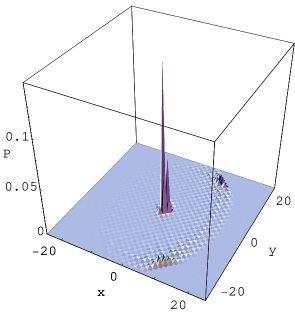
Figure 4: The probability $P(x,y,t;\phi_{R})$ of the quantum walk whose wave function is determined by the matrix $A_{4}$ with $p=1/3$ and $q=2/3$. A sharp distribution at the origin is observed similarly as in the case of the Grover walk.