How to measure squeezing and entanglement of Gaussian states without homodyning

Abstract

We propose a scheme for measuring the squeezing, purity, and entanglement of Gaussian states of light that does not require homodyne detection. The suggested setup only needs beam splitters and single-photon detectors. Two-mode entanglement can be detected from coincidences between photodetectors placed on the two beams.

The recent rapid development of quantum information theory has largely stimulated research on nonclassical states of light, with the main focus on the generation of entangled states of light that are required for tasks such as quantum teleportation, dense coding, or certain types of quantum key distribution protocols. A particularly promising approach consists in processing quantum information with continuous variables Braunsteinbook , where the quantum information is encoded into two conjugate quadratures of the quantized mode of the optical field. The main advantage of this approach is that many protocols can be implemented by processing squeezed light into linear optical interferometers followed by measurements with highly efficient photodiodes Braunsteinbook . Such experiments can be described in terms of Gaussian states which thus play a central role in continuous-variable quantum information processing. In particular, squeezed Gaussian states provide the necessary source of entanglement. The squeezing is usually observed with the use of a balanced homodyne detector, where the signal beam is combined with a strong local oscillator (LO) providing a phase reference Bachorbook . The observed quadrature fluctuations depend on the relative phase between the LO and the signal. The maximal squeezing of the signal then corresponds to the minimal observed quadrature variance.

Given that quadrature squeezing is inherently a phase-sensitive phenomenon, one would expect that it may not be possible to determine the squeezing properties without an external phase reference (LO). In this paper, we show that, surprisingly, a phase-insensitive device is sufficient provided that we can a priori assume that the optical mode is in a Gaussian state. The setup we suggest consists in beam splitters with variable splitting ratios, phase shifters, and photodetectors with single-photon sensitivity (e.g., avalanche photodiodes). It can also be extended to estimate the squeezing of multimode Gaussian states. In particular, a variation of our setup is capable of measuring the degree of entanglement of a two-mode Gaussian state, namely the logarithmic negativity Eisertthesis ; Vidal02 . Besides the determination of squeezing and entanglement, our setup can also be used to measure the purity of Gaussian states Kim02 . In addition, the detectors need not be perfect and an efficiency $\eta<1$ can easily be compensated by proper data processing.

Our scheme works for an arbitrary number of modes $N$ and is economic with respect to $N$ in the sense that the number of measured parameters is only linear in $N$ while the full tomography of Gaussian states revealing the whole covariance matrix would require the measurement of $\propto N^{2}$ parameters. In this context, it is related to several recent proposals on how to directly measure the purity, overlap, and entanglement of quantum states without full state reconstruction Filip02 ; Horodecki02 ; Ekert02 ; Hendrych03 . It is also reminiscent of the photon-number distribution measurement scheme using a photodetector without single-photon resolution as proposed in Ref. Mogilevtsev98 .

Preliminaries.

Let us begin with introducing the necessary notation and definitions. Let $r=(x_{1},p_{1},\ldots,x_{k},p_{k},\ldots,x_{N},p_{N})$ be the vector of conjugate quadratures of $N$ modes which satisfy the canonical commutation relations $[x_{j},p_{k}]=i\delta_{jk}$. The Gaussian state is fully described by the vector of mean values $\xi_{j}=\langle r_{j}\rangle$ and the covariance matrix

$$\gamma_{jk}=\langle\Delta r_{j}\Delta r_{k}\rangle+\langle\Delta r_{k}\Delta r_{j}\rangle,$$ (1)

where $\Delta r_{j}=r_{j}-\xi_{j}$. The quantum state of the optical field can be fully characterized by a $s$-parametrized quasidistribution which provides phase-space representation of the quantum state. For our purposes, it is convenient to utilize the Husimi Q-function. The Q-function of an $N$-mode Gaussian state is the Gaussian distribution Perinabook

$$Q(r)=\frac{\pi^{-N}}{\sqrt{\det(\gamma+I)}}\exp\left[-(r-\xi)^{T}(\gamma+I)^{-1}(r-\xi)\right],$$ (2)

where $I$ is the identity matrix. The squeezing properties do not depend on $\xi$ and are fully described by $\gamma$. The maximal observable squeezing, i.e. the minimal quadrature variance, is called the generalized squeezing variance $\lambda$ and can be determined as the minimal eigenvalue of the covariance matrix Simon94 ,

$$\lambda=\min[\mathrm{eig}(\gamma)].$$ (3)

The purity of the mixed state with density matrix $\rho$ is defined as $\mathcal{P}=\mathrm{Tr}[\rho^{2}]$. For a Gaussian state with covariance matrix $\gamma$, one obtains Kim02

$$\mathcal{P}=[\det(\gamma)]^{-1/2}.$$ (4)

Figure 1: Direct measurement of a Gaussian state with the use of a photodetector PD with single-photon sensitivity, preceeded by a beam splitter BS of transmittance $T$. (a) Single-copy scheme for $\xi=0$. (b) Two-copy scheme for $\xi\neq 0$.

Single-mode case.

For the sake of simplicity, we first illustrate the procedure on single-mode Gaussian states ($N=1$). Consider the setup depicted in Fig. 1(a). The input mode impinges on a beam splitter BS with tunable transmittance $T$, and the output mode is measured by a photodetector PD with efficiency $\eta$ that is sensitive to single photons (no single-photon resolution is needed). We assume that this realistic detector can be modeled as a beam splitter with transmittance $\eta$ followed by an ideal detector that performs a dichotomic measurement described by the POVM elements $\Pi_{0}=|0\rangle\langle 0|$ and $\Pi_{1}=\openone-\Pi_{0}$. (In what follows, we assume that the detector is ideal and $\eta$ can be taken into account by substituting $T\rightarrow\eta T$.) The probability of no-click of an ideal detector PD is given by $P=\mathrm{Tr}[\rho\Pi_{0}]=\langle 0|\rho|0\rangle=2\pi Q(0)$, so that inserting $r=0$ into Eq. (2) yields

$$P=\frac{2}{\sqrt{\det(\gamma^{\prime}+I)}}\exp\left[-\xi^{\prime T}(\gamma^{\prime}+I)^{-1}\xi^{\prime}\right].$$ (5)

where $\gamma^{\prime}$ and $\xi^{\prime}$ are, respectively, the covariance matrix and the displacement vector of the beam impinging on the photodetector.

Suppose that we set the beam splitter transmittance to the value $T_{j}$. The covariance matrix $\gamma^{\prime}$ of the state after passing the beam splitter reads $\gamma^{\prime}=T_{j}\gamma+(1-T_{j})I$. Similarly, the coherent signal is damped to $\xi^{\prime}=\sqrt{T_{j}}\xi$. On inserting $\gamma^{\prime}$ and $\xi^{\prime}$ into Eq. (5), we obtain

$$P_{j}=\frac{2}{[\det(\tilde{\gamma}_{T_{j}})]^{1/2}}\exp\left(-T_{j}\xi^{T}\tilde{\gamma}_{T_{j}}^{-1}\xi\right).$$ (6)

where $\tilde{\gamma}_{T_{j}}=T_{j}\gamma+(2-T_{j})I$. We thus find that $P_{j}$ depends on $T_{j}$ and four parameters of the state: $\det\gamma$, $\mathrm{Tr}(\gamma)$, $g_{1}=\xi_{1}^{2}\gamma_{22}+\xi_{2}^{2}\gamma_{11}-2\gamma_{12}\xi_{1}\xi_{2}$, and $g_{2}=\xi_{1}^{2}+\xi_{2}^{2}$. This immediately suggests that if we measure $P_{j}$ for at least four different $T_{j}$’s, we might be able to reconstruct the values of these four parameters by solving a system of nonlinear equations. However, numerical simulations reveal that the inversion of these highly nonlinear equations typically leads to extremely large fluctuations of the estimated parameters even for a very large number of measurements for each setting $T_{j}$.

Fortunately, in the important case where the displacement vector is zero ($\xi=0$), the scheme provides reliable and well-behaved estimates of these parameters since formula (6) then simplifies to

$$\det\tilde{\gamma}_{T_{j}}=T^{2}\det(\gamma)+T(2-T)\mathrm{Tr}(\gamma)+(2-T)^{2}=4P_{j}^{-2}.$$ (7)

This results in a system of linear equations for $\det(\gamma)$ and $\mathrm{Tr}(\gamma)$. If measurements for two different transmittances $T_{1}$ and $T_{2}$ are performed and the observed probabilities of no-click are $P_{1}$ and $P_{2}$, then the system of Eqs. (7) can easily be solved and yields

$$\mathrm{Tr}(\gamma)=\frac{2}{T_{2}-T_{1}}\left(\frac{T_{2}}{T_{1}P_{1}^{2}}-\frac{T_{1}}{T_{2}P_{2}^{2}}\right)+2-\frac{2}{T_{1}}-\frac{2}{T_{2}},$$ (8)

$$\det(\gamma)=\frac{2}{T_{1}-T_{2}}\left(\frac{2-T_{2}}{T_{1}P_{1}^{2}}-\frac{2-T_{1}}{T_{2}P_{2}^{2}}\right)+\frac{(2-T_{1})(2-T_{2})}{T_{1}T_{2}}.$$ (9)

Let us investigate what can be extracted from the knowledge of $\mathrm{Tr}(\gamma)$ and $\det(\gamma)$. As noted above, the squeezing properties of the Gaussian state, namely the generalized squeezing variance $\lambda$, can be determined from the eigenvalues of $\gamma$, cf. Eq. (3). For a single-mode state, $\gamma$ is symmetric $2\times 2$ matrix and its eigenvalues can be expressed in terms of $\det(\gamma)$ and $\mathrm{Tr}(\gamma)$, which are both determined by the present method. We find that

$$\lambda=\frac{1}{2}\left[\mathrm{Tr}(\gamma)-\sqrt{\mathrm{Tr}^{2}(\gamma)-4\det(\gamma)}\right].$$ (10)

Moreover, since our method provides an estimate of $\det{\gamma}$, we can also determine the purity from Eq. (4).

If $\xi\neq 0$, our scheme is still usable provided that we can perform a collective measurement on two copies of the state, as depicted in Fig. 1(b). The two input modes $A_{I}$ and $A_{II}$ prepared in identical Gaussian state interfere on a balanced beam splitter. In the Heisenberg picture, the annihilation operators of the output modes $A_{+}$ and $A_{-}$ are linear combinations of those of the input modes, $a_{\pm}=2^{-1/2}(a_{I}\pm a_{II})$. The covariance matrix of mode $A_{-}$ is equal to $\gamma$ Browne03 but the coherent signal in $A_{-}$ vanishes due to the destructive interference, $\xi_{-}=0$. As shown in Fig. 1(b), the mode $A_{-}$ is subsequently sent to a direct measurement setup identical to that shown in Fig. 1(a).

Multimode case.

We now extend this procedure to multimode Gaussian states. A reliable operation again requires two copies $A_{I}$ and $A_{II}$. Essentially, we use in parallel $N$ setups such as shown in Fig. 1(b). We combine each pair of modes $A_{I,k}$ and $A_{II,k}$, with $k=1,\ldots,N$, on a balanced beam splitter. Each “minus” mode $A_{-,k}$, with $\xi=0$, is then sent to a beam splitter of transmittance $T_{j}$ followed by a photodetector. We measure the probability $P_{j}=2^{N}/(\det\tilde{\gamma}_{T_{j}})^{1/2}$ that none of the $N$ detectors clicks. For an $N$-mode state, the determinant of $\tilde{\gamma}_{T}=T\gamma+(2-T)I$ can be expanded as

$$\det(\tilde{\gamma}_{T})=\sum_{n=1}^{2N}T^{n}(2-T)^{2N-n}f_{n}(\gamma)+(2-T)^{2N},$$ (11)

where $f_{n}(\gamma)$ is an homogeneous polynomial of $n$th order in the matrix elements of $\gamma$, e.g., $f_{2N}(\gamma)=\det(\gamma)$ and $f_{1}(\gamma)=\mathrm{Tr}(\gamma)$. The probability $P_{j}$ thus depends on $T_{j}$ and the $2N$ parameters $f_{n}(\gamma)$. If we measure $P_{j}$ for $2N$ (or more) different transmittances $T_{j}$’s, then we can determine the parameters $f_{n}$ of the Gaussian state by solving a system of linear equations

$$\sum_{n=1}^{2N}T_{j}^{n}(2-T_{j})^{2N-n}f_{n}(\gamma)=2^{2N}P_{j}^{-2}-(2-T_{j})^{2N}.$$ (12)

Once we know $f_{n}(\gamma)$, we can determine the generalized squeezing variance $\lambda$ as the smallest root of the characteristic polynomial $\det(\lambda I-\gamma)=0$. It can be seen from Eq. (11) that the parameters $f_{j}(\gamma)$ are the coefficients of this characteristic polynomial, and we have

$$\lambda^{2N}+\sum_{k=0}^{2N-1}\lambda^{k}(-1)^{k}f_{2N-k}(\gamma)=0.$$ (13)

We can also determine the purity of the $N$-mode Gaussian state from $f_{2N}(\gamma)$ with the help of formula (4).

Entanglement detection.

In the context of quantum information processing with continuous variables, the entanglement properties of Gaussian states deserve particular attention. It has been shown that a two-mode Gaussian state is separable iff it has a positive partial transpose Duan00 ; Simon00 . This property can easily be checked if one knows the covariance matrix

$$\gamma_{AB}=\left(\begin{array}[]{cc}\gamma_{A}&\sigma_{AB}\\ \sigma_{AB}^{T}&\gamma_{B}\end{array}\right)$$ (14)

of the bipartite state, where $\gamma_{A}$ and $\gamma_{B}$ are the covariance matrices of modes $A$ and $B$, respectively, while $\sigma_{AB}$ captures the intermodal correlations. Moreover, analytical formulas for several entanglement monotones that measure the entanglement of Gaussian states have been given in the literature Vidal02 ; Giedke03 . A particularly simple formula has been obtained for the logarithmic negativity $E_{\mathcal{N}}$ of an arbitrary Gaussian state. To calculate $E_{\mathcal{N}}$, we must determine the symplectic spectrum of the covariance matrix of the partially transposed state $\rho_{AB}^{T_{A}}$. As shown in Ref. Vidal02 , the symplectic eigenvalues are the two positive roots $\zeta_{1}\geq\zeta_{2}>0$ of the biquadratic equation

$$\zeta^{4}-(\det\gamma_{A}+\det\gamma_{B}-2\det\sigma_{AB})\zeta^{2}+\det\gamma_{AB}=0.$$ (15)

The solution of Eq. (15) yields

$$\zeta_{2}^{2}=\frac{1}{2}\left(D-\sqrt{D^{2}-4\det\gamma_{AB}}\right),$$ (16)

where $D=\det\gamma_{A}+\det\gamma_{B}-2\det\sigma_{AB}$. The two-mode Gaussian state is entangled if and only if $\zeta_{2}<1$. In this case, we have $E_{\mathcal{N}}=-\log(\zeta_{2})$, while $E_{\mathcal{N}}=0$ otherwise. The condition $\zeta_{2}<1$ implies the necessary and sufficient entanglement condition $D>1+\det\gamma_{AB}$ Simon00 ; Giedke01 , which explicitly reads,

$$\det\gamma_{A}+\det\gamma_{B}-2\det\sigma_{AB}>1+\det\gamma_{AB}.$$ (17)

With the use of the method proposed in the present paper we can measure $\det\gamma_{AB}$, $\det\gamma_{A}$, and $\det\gamma_{B}$. An upper bound on $\det\sigma_{AB}$ in terms of these determinants can be derived from the condition that the symplectic eigenvalues $\tilde{\zeta}_{j}$ of the covariance matrix $\gamma_{AB}$ must be greater or equal to one Giedke01 . The lower eigenvalue $\tilde{\zeta}_{2}$ is given by Eq. (16), where $D$ is replaced with $D^{\prime}=\det\gamma_{A}+\det\gamma_{B}+2\det\sigma_{AB}$. The condition $\tilde{\zeta}_{2}^{2}\geq 1$ yields

$$2\det\sigma_{AB}\leq\det\gamma_{AB}+1-\det\gamma_{A}-\det\gamma_{B}.$$ (18)

This, in turn, implies an upper bound on the lower symplectic eigenvalue $\zeta_{2}$ of the covariance matrix of $\rho_{AB}^{T_{A}}$. On inserting the upper bound on $2\det\sigma_{AB}$ given by Eq. (18) into Eqs. (16) and (17) we find that $\zeta_{2}<1$, so that the state is entangled when

$$\det\gamma_{A}+\det\gamma_{B}>1+\det\gamma_{AB}$$ (19)

holds. Inequality (19) is thus a sufficient condition for entanglement, but it is not necessary as some Gaussian entangled states are not detected by this test. The main advantage of this test is that all determinants appearing in Eq. (19) can be determined by local measurements supplemented with classical communication between $A$ and $B$. Moreover, if we can a priori assume that $\xi=0$, then measurements on a single copy of $\rho_{AB}$ suffice.

If we now want to exactly determine $E_{\mathcal{N}}$, we also need a scheme to measure $\det\sigma_{AB}$. This can be accomplished provided that we can perform joint measurements on several copies of the state $\rho_{AB}$. Unlike the previous one, this scheme requires joint nonlocal measurements on modes $A$ and $B$, and it involves several steps as schematically illustrated in Fig. 2. Using the scheme of Fig. 2(b), we can measure the determinants of the covariance matrices $\gamma_{+}$ and $\gamma_{-}$ of modes $A_{+}$ and $A_{-}$ that are linear combinations of the modes $A$ and $B$, $a_{\pm}=(a\pm b)/\sqrt{2}$. After a simple algebra, we find that

$$\det(\sigma_{AB}+\sigma_{AB}^{T})=2\det\gamma_{+}+2\det\gamma_{-}-\det(\gamma_{A}+\gamma_{B}).$$ (20)

In order to determine $\det(\gamma_{A}+\gamma_{B})$, we have to carry out a joint measurement on two independent copies of the two-mode state, as depicted in Fig. 2(c). By mixing the modes $A_{1}$ and $B_{2}$ on a balanced beam splitter, we prepare an output single-mode state with covariance matrix $\gamma_{A+B}\equiv(\gamma_{A}+\gamma_{B})/2$. Recall that the modes $A_{1}$ and $B_{2}$ belong to two independent copies of the two-mode state $\rho_{AB}$, hence $A_{1}$ and $B_{2}$ are uncorrelated. After the measurement of $\det\gamma_{+}$, $\det\gamma_{-}$, and $\det\gamma_{A+B}$, we calculate $\det(\sigma_{AB}+\sigma_{AB}^{T})$ from Eq. (20). It holds that $\det(\sigma_{AB}+\sigma_{AB}^{T})\leq 4\det\sigma_{AB}$ and the equality is achieved when $\sigma_{AB}$ is symmetric. The matrix $\sigma_{AB}$ can be brought to a symmetric form by applying a local phase shift $\exp(i\phi b^{\dagger}b)$ to the mode $B$ using the phase shifter PS in Fig. 2. This transforms $\sigma_{AB}$ to $\sigma_{AB}U(\phi)$ where

$$U(\phi)=\left(\begin{array}[]{cc}\cos\phi&\sin\phi\\ -\sin\phi&\cos\phi\end{array}\right).$$

To determine the phase shift $\phi$ that symmetrizes $\sigma_{AB}$, we measure $y_{\phi}\equiv\det[\sigma_{AB}U(\phi)+U^{T}(\phi)\sigma_{AB}^{T}]$ for three different phases $\phi=0$, $\pi/4$, and $\pi/2$. It can be shown that

$$y_{\phi}=y_{0}\cos^{2}\phi+y_{\pi/2}\sin^{2}\phi+\tilde{y}_{\pi/4}\sin(2\phi),$$

where $\tilde{y}_{\pi/4}=y_{\pi/4}-(y_{0}+y_{\pi/2})/2$. The value of $\det\sigma_{AB}$ can be found as the maximum of $y_{\phi}$ over $\phi$ which yields

$$\det\sigma_{AB}=\frac{1}{8}\left[y_{0}+y_{\pi/2}+\sqrt{(y_{0}-y_{\pi/2})^{2}+4\tilde{y}_{\pi/4}^{2}}\,\right].$$

This finally provides all the information required for the exact calculation of the logarithmic negativity $E_{\mathcal{N}}$.

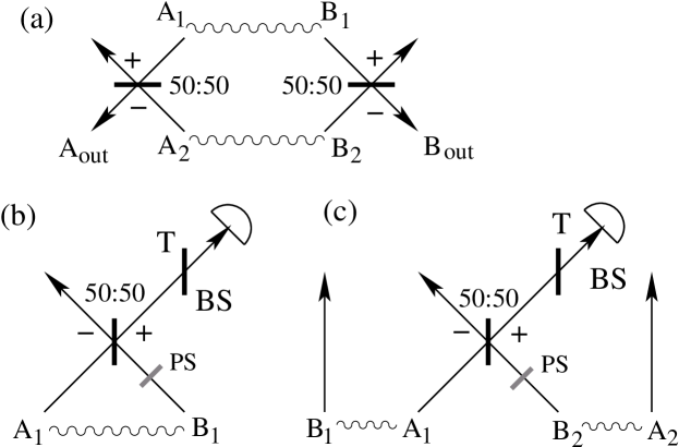
Figure 2: Direct measurement of the intermodal correlations $\det\sigma_{AB}$ of a two-mode Gaussian state. (a) Preparation of states with zero displacement $\xi=0$ needed for steps (b) and (c). (b) Measurement of $\det\gamma_{+}$ ($\det\gamma_{-}$ is measured similarly). (c) Measurement of $\det\gamma_{A+B}$.

In summary, we have proposed a scheme for the direct measurement of the squeezing, purity, and entanglement of Gaussian states that does not require homodyne detection but only needs beam splitters and photodetectors with single-photon sensitivity. The scheme generally requires joint measurements on two copies of the state, but single-copy measurements suffice if it is a priori known that the mean (or coherent) values of the quadratures vanish, which is, e.g., the case of the squeezed and entangled states generated by spontaneous parametric downconversion. We have shown that, based on Eq. (19), the present method can be used to assess the entanglement of $1\times 1$ Gaussian states by means of local measurements, without employing any local oscillator or interferometric schemes. Given the simplicity of the suggested setup, the prospects for an experimental realization in a near future look very good.

Note added: The sufficient condition on entanglement [Eq. (19)] has recently and independently been derived by Adesso et al. Adesso03 . Besides the lower bound on $E_{\mathcal{N}}$ linked to Eq. (19), an upper bound on $E_{\mathcal{N}}$ expressed in terms of the determinants of $\gamma_{A}$, $\gamma_{B}$, and $\gamma_{AB}$ was also derived in Ref. Adesso03 . Remarkably, these two bounds are typically very close to each other, so the knowledge of the determinants of the covariance matrices provides quite precise quantitative information on the entanglement, making the direct measurement procedure particularly powerful.

We acknowledge financial support from the Communauté Française de Belgique under grant ARC 00/05-251, from the IUAP programme of the Belgian government under grant V-18, from the EU under projects RESQ (IST-2001-37559) and CHIC (IST-2001-32150). JF also acknowledges support from the grant LN00A015 of the Czech Ministry of Education.

References

- (1)
- (2) S.L. Braunstein and A.K. Pati, Quantum Information with Continuous Variables, (Kluwer Academic, Dordrecht, 2003).
- (3) For a review on experiments with squeeezed light, see e.g. H.-A. Bachor, A Guide to Experiments in Quantum Optics, (John Wiley & Sons, 1998).
- (4) J. Eisert, Ph.D. Thesis, University of Potsdam (2001).
- (5) G. Vidal and R. F. Werner, Phys. Rev. A 65, 032314 (2002).
- (6) M.S. Kim, J. Lee, and W.J. Munro, Phys. Rev. A 66, 030301 (2002); M.G.A. Paris, F. Illuminati, A. Serafini, and S. De Siena, Phys. Rev. A 68, 012314 (2003).
- (7) R. Filip, Phys. Rev. A 65, 062320 (2002).
- (8) A.K. Ekert, C.M. Alves, D.K.L. Oi, M. Horodecki, P. Horodecki, and L.C. Kwek, Phys. Rev. Lett. 88, 217901 (2002).
- (9) M. Hendrych, M. Dušek, R. Filip, and J. Fiurášek, Phys. Lett. A 310, 95 (2003).
- (10) P. Horodecki and A. Ekert, Phys. Rev. Lett. 89, 127902 (2002); P. Horodecki, Phys. Rev. Lett. 90, 167901 (2003).
- (11) D. Mogilevtsev, Opt. Commun. 156, 307 (1998).
- (12) J. Peřina, Quantum Statistics of Linear and Nonlinear Optical Phenomena (Kluwer, Dordrecht, 1991).
- (13) R. Simon, N. Mukunda and B. Dutta, Phys. Rev. A 49, 1567 (1994).
- (14) D.E. Browne, J. Eisert, S. Scheel, and M.B. Plenio, Phys. Rev. A 67, 062320 (2003).
- (15) L.M. Duan, G. Giedke, J.I. Cirac, and P. Zoller, Phys. Rev. Lett. 84, 2722 (2000).
- (16) R. Simon, Phys. Rev. Lett. 84, 2726 (2000).
- (17) G. Giedke et al., Phys. Rev. Lett. 91, 107901 (2003); M.M. Wolf et al., quant-ph/0306177.
- (18) G. Giedke, L.M. Duan, J.I. Cirac, and P. Zoller, Quant. Inf. Comp. 1, 79 (2001).
- (19) G. Adesso, A. Serafini, and F. Illuminati, quant-ph/0310150.