Average fidelity between random quantum states

Abstract

We analyze mean fidelity between random density matrices of size $N$, generated with respect to various probability measures in the space of mixed quantum states: Hilbert-Schmidt measure, Bures (statistical) measure, the measures induced by partial trace and the natural measure on the space of pure states. In certain cases explicit probability distributions for fidelity are derived. Results obtained may be used to gauge the quality of quantum information processing schemes.

e-mail: karol@cft.edu.pl    sommers@theo-phys.uni-essen.de

I Introduction

Modern applications of quantum theory renewed interest in characterization of the set of mixed quantum states. It is often necessary to quantify, how a certain mixed state may be approximated by another one. For this purpose one may use various distances defined in the space of mixed quantum states, e.g. the trace distance, the Hilbert-Schmidt (HS) distance and the Bures distance Bu69 . The latter distance, is a function of fidelity Jo94 , and may be considered as a generalization of the overlap between pure states Uh76 . Fidelity between a pair of two mixed states is equal to unity if and only if they do coincide. Optimal fidelity between the input and the output states are used to characterize the quality of a cloning algorithm BH96 ; Ce00 .

In various quantum problems one computes the mean fidelity, averaging over a certain ensemble of states. Analyzing dynamics of quantum chaotic systems one studies the fidelity between a given initial state and its image under the action of the quantum map Pr02 . To extract global information on the entire system one averages this quantity over the natural, Fubini–Study (FS) measure on the space of initial pure states. Mean fidelity between two images of a random pure state obtained by the action of a certain unitary operation and a certain irreversible, contracting superoperator $\cal E$ was found by Bowdery et al. BOSJ01 for qubits and by Nielsen Ni02 for the more general case of $N$ dimensional states. Another expression for the average gate fidelity was recently derived by Bagan et al. BBMT03 , in which the nontrivial term was shown to be proportional to the mean value of the Hilbert–Schmidt scalar product $\langle{\rm Tr}\gamma_{i}{\cal E}(\gamma_{i})\rangle_{i}$ of the $SU(N)$ generators $\gamma_{i}$ and their images ${\cal E}(\gamma_{i})$, averaged over all of them, $i=1,\dots,N^{2}-1$.

In this work we study a complementary problem and analyze mean fidelity $\langle F\rangle$ between two independent, random states. Such a problem may be interesting from a practical point of view: The average fidelity may serve as reference value by analyzing the mean (maximal/minimal) fidelity achieved in a certain protocol of quantum cloning. For instance, if the measured (computed) fidelity between a certain pair of one–qubit mixed states only slightly exceeds the average value, one should not conclude that these states are more correlated than two generic, random mixed states.

In this way we are in position to propose a general tool measuring the quality of a given theoretical scheme of quantum information processing or its experimental realization. Let $\tilde{F}$ denote the mean fidelity between the state obtained in an analyzed cloning protocol and the target state. Then the quality of the protocol may be gauged by a dimensionless coefficient $\alpha=[{\tilde{F}}-\langle F\rangle]/\sqrt{\langle F^{2}\rangle-\langle F\rangle^{2}}$, where $\langle F\rangle$ denotes the average over an appropriate ensemble of random density matrices.

We are also interested in the probability distribution $P(F)$. Two averaging schemes should be distinguished. In the symmetric case, both states are drawn at random according to the same measure (e.g. both pure states or both mixed states generated with respect to the same probability distribution). In the non-symmetric case, both probability distributions are different: in particular we study the mean fidelity between a random pure state and a random mixed state, generated with respect to a specified measure.

Let us emphasize in this place that there exists no single, naturally distinguished probability measure in the set of mixed quantum states Ha98 ; ZS01 ; SZ03b . Guessing a mixed state of size $N$ at random we might use additional information, if available. For instance, knowing that the mixed state has arisen by the partial tracing over a $K$ dimensional environment, the induced measure ZS01 should be used. In particular, if the size of the environment $K$ and the size $N$ of the system are equal, then the measure induced by partial trace coincides with the Hilbert-Schmidt measure. Without any information concerning the random state whatsoever, it will be legitimate to make use of the Bures measure, related to the Jeffrey’s prior, statistical distance and the distinguishability.

The paper is organized as follows. In section 2 we review the basic properties of fidelity, while in section 3 we introduce the necessary measures in the set of mixed quantum states of size $N$. Mean fidelity between pure and mixed states are analyzed in section 4. Main results of this work are presented in section 5, in which we compute the mean fidelity, averaged over two independent random mixed states, generated with respect to an arbitrary induced measure, labeled by the size $K$ of the environment. The probability distribution for fidelity between a random pure state and a random mixed state distributed according to the Bures measure is computed in Appendix B, while the derivation of the generating functions for the moments of the root fidelity for two mixed states of arbitrary $N$ generated independently according to an induced measure is postponed to Appendix A.

II Fidelity

Let ${\cal M}_{N}$ denote the set of all mixed quantum states of size $N$. It contains all Hermitian, semipositive definite matrices of size $N$, which are trace normalized,

$${\rm Tr}\rho=1\ .$$ (1)

We are going to consider two distances in this set: the Hilbert-Schmidt distance

$$D_{HS}(\rho_{1},\rho_{2})=\sqrt{{\rm Tr}[(\rho_{1}-\rho_{2})^{2}]}.$$ (2)

and the Bures distance Bu69 ; Uh76 ,

$$\bigl{(}D_{B}(\rho_{1},\rho_{2})\bigr{)}^{2}=2-2\ \mbox{Tr}\sqrt{\sqrt{{\rho}_{1}}{\rho}_{2}\sqrt{{\rho}_{1}}}=2-2\sqrt{F(\rho_{1},\rho_{2})}\ .$$ (3)

respectively.

The Bures distance is distinguished by several remarkable properties: for pure states it agrees with the natural, Fubini-Study distance, while in the space of diagonal density matrices it induces the statistical (Fisher) distance PS96 . The Bures distance is a function of fidelity Jo94 : .

$$F(\rho_{1},\rho_{2}):=\Bigl{[}\mbox{Tr}\sqrt{\sqrt{{\rho}_{1}}{\rho}_{2}\sqrt{{\rho}_{1}}}\Bigr{]}^{2}.$$ (4)

This quantity is sometimes called Uhlmann transition probability Uh76 , since for a pair of pure states it reduces to the squared overlap, $F={\rm Tr}\rho_{1}\rho_{2}=|\langle\psi_{1}|\psi_{2}\rangle|^{2}$

Fidelity enjoys several important properties Jo94 : it is a symmetric, non-negative, continuous, concave function of both states, unitarily invariant, equal to unity if and only if both states do coincide. Therefore it becomes an important tool to characterize the closeness of any two mixed states, often used in modern applications of quantum mechanics (see e.g. NC00 ). The only disadvantage consists in computing it explicitly: to find the fidelity one needs to diagonalize the density matrices, but more importantly, the fidelity stays being a function of the eigenvectors.

Apart of the fidelity $F$, we will also use the square root fidelity $\sqrt{F}$. Also this quantity satisfies several appealing properties NC00 and in certain cases its probability distribution is easier to compute then $P(F)$. Furthermore the quantity $\arccos[\sqrt{F(\sigma,\rho)}]$ has a clear geometric interpretation as Bures angle in the space of mixed states equipped with the Bures metric. It is equal to the geodesic Riemannian distance between both mixed states Uh92 ; Uh95 , and in the case of pure states it coincides with the Fubini–Study distance.

Computation of fidelity is much simpler for $N=2$. To derive an explicit formula for fidelity we use first steps of the calculation of the Bures distance presented by Hübner Hu92 . Any two-by-two matrix $A$ obeys the characteristic equation

$$A^{2}-A\mbox{Tr}A+{\mathbbm{1}}\det{A}=0\ .$$ (5)

Taking the trace we obtain

$$(\mbox{Tr}A)^{2}=\mbox{Tr}A^{2}+2\det{A}\ .$$ (6)

Let us now set $A=\sqrt{\sqrt{{\rho}_{1}}{\rho}_{2}\sqrt{{\rho}_{1}}}$, so that Tr$A^{2}={\rm Tr}{\rho}_{1}{\rho}_{2}$ and $\det A=\sqrt{\det{{\rho}_{1}}\det{{\rho}_{2}}}$. Let $(p_{1},p_{2})$ denote the spectrum of a state $\rho$. Hence $1=(p_{1}+p_{2})^{2}={\rm Tr}\rho^{2}+2\det\rho$ and $2\det\rho=1-{\rm Tr}\rho^{2}$. Substituting this into Eq. (6) we obtain

$$F(\rho_{1},\rho_{2})=({\rm Tr}A)^{2}=\mbox{Tr}\rho_{1}\rho_{2}+\sqrt{(1-\mbox{Tr}\rho_{1}^{2})(1-\mbox{Tr}\rho_{2}^{2})}\ .$$ (7)

III Measures in the space of mixed quantum states

Random quantum states may be generated according to different measures, and it is hardly possible to distinguish the unique probability measure in the set of density matrices. Usually one considers product measures, which may be factorized Ha98 ; ZS01

$${\rm d}\mu_{x}={\rm d}\nu_{x}(\lambda_{1},\lambda_{2},...,\lambda_{N})\times{\rm d}h\ .$$ (8)

The second factor d$h$, determining the distribution of the eigenvectors of the density matrix, is the unique, unitarily invariant Haar measure on $U(N)$, while the first factor depends only on the eigenvalues $\lambda_{i}$ of $\rho$ and may be chosen by an arbitrary probability distribution d$\nu_{x}=P_{x}({\vec{\lambda}})d^{N}\lambda$. The joint probability distribution is defined on the $(N-1)$ dimensional simplex $\Delta_{N-1}$, which contains all vectors of non-negative entries summing to unity.

The Hilbert-Schmidt measure, induced by the Hilbert-Schmidt metric, is defined by the following joint probability distribution Ha98 ; ZS01

$$P_{\rm HS}^{(N)}({\vec{\lambda}})=\frac{\Gamma(N^{2})\ \delta\bigl{(}\sum_{j=1}^{N}\lambda_{j}-1\bigr{)}}{\prod_{j=0}^{N-1}\Gamma(N-j)\Gamma(N-j+1)}\prod_{i<j}^{N}(\lambda_{i}-\lambda_{j})^{2}.$$ (9)

The Bures metric leads to the Bures measure in the simplex of eigenvalues

$$P_{\rm B}^{(N)}({\vec{\lambda}})=\frac{2^{N^{2}-N}\ \Gamma(N^{2}/2)}{\pi^{N/2}\ \Gamma(1)...\Gamma(N+1)}\frac{\delta\bigl{(}\sum_{j=1}^{N}\lambda_{j}-1\bigr{)}}{\sqrt{\lambda_{1}\lambda_{2}\cdots\lambda_{N}}}\prod_{i<j}\frac{(\lambda_{i}-\lambda_{j})^{2}}{\lambda_{i}+\lambda_{j}}.$$ (10)

This probability distribution was derived by Hall Ha98 , while the normalization constants where found in Sl99b for $N=3,4,5$ and in SZ03 for an arbitrary $N$.

Is is also instructive to consider a family of measures in the space of mixed states of size $N$ induced by the Haar measure on the unitary group $U(NK)$. The integer parameter $K$, used to label the measure $\mu_{N,K}$, represents the size of an ancilla. A mixed state of size $N$ may be obtained by tracing a certain random pure state $|\Phi\rangle$ of size $NK$ over the $K$–dimensional ancilla, $\rho={\rm T}_{K}\bigl{(}|\Phi\rangle\langle\Phi|\bigr{)}$. Representing the pure state $|\Phi\rangle$ in an arbitrary product basis $|i,j\rangle=|i\rangle\otimes|j\rangle$ where $i=1,...,N$ and $j=1,...,K$ we obtain $|\Phi\rangle=\Phi_{ij}|i,j\rangle$. The rectangular matrix of coefficients $\Phi_{ij}$ of size $N\times K$ allows us to write the reduced state as $\rho=\Phi\Phi^{\dagger}$. If matrices $\Phi$ are random, the matrices $\rho$ constructed in such a way are called Wishart matrices. The probability distribution of eigenvalues of $\rho$ reads Lu78 ; LS88 ; Pa93 ; ZS01

$$P_{\mu_{N,K}}({\vec{\lambda}})=\frac{\Gamma(KN)\delta\bigl{(}\sum_{j=1}^{N}\lambda_{j}-1\bigr{)}}{\prod_{j=0}^{N-1}\Gamma(K-j)\Gamma(N-j+1)}\prod_{i}\lambda_{i}^{K-N}\prod_{i<j}(\lambda_{i}-\lambda_{j})^{2}$$ (11)

and for $K=N$ reduces to the Hilbert-Schmidt measure (9). In the above equation the inequality $K\geq N$ is assumed and this case is called the Wishart case. If this is not the case, (the so–called anti–Wishart case YZ02 ; JN03 ) induced measures with $K<N$ are singular, since they are supported by the subspace of states of submaximal rank $K$ which belongs to the boundary of ${\cal M}_{N}$. In particular, the measure $\mu_{N,1}$ is just the natural Fubini–Study measure on the space of pure states in ${\cal H}_{N}$, since the partial trace over an $1$–dimensional ancilla does not change the pure state.

Interestingly, in the one–qubit case, for $K=3/2$, the induced measure (11) reduces to the Bures measure (10),

$$P_{\rm B}^{(2)}({\vec{\lambda}})=P_{\mu_{2,3/2}}({\vec{\lambda}})$$ (12)

Although such a coincidence occurs for an non-integer value of the dimensionality of the environment, and seems not to have any physical meaning, it will help us to obtain some results for the Bures measure by analytical continuation in $K$. Unfortunately this trick works only in the $N=2$ case, for which $\lambda_{1}+\lambda_{2}=1$, so the denominator under the product in the distribution (10) is trivially equal to unity.

We are going to study mean fidelity $\langle F\rangle$ with respect to different measures. Let $\langle F\rangle_{\mu}$ denote the homogeneous case, in which both arguments of fidelity are random mixed states, distributed independently with respect to the same probability measure $\mu$. In a more general case we may average over two different measures and such averages will be denoted by $\langle F\rangle_{\mu_{1}}^{\mu_{2}}$. Since fidelity is symmetric $F(\rho_{1},\rho_{2})=F(\rho_{2},\rho_{1})$, we have $\langle F\rangle_{\mu_{1}}^{\mu_{2}}=\langle F\rangle_{\mu_{2}}^{\mu_{1}}$.

An analogous notation will be also used to label probability distributions for fidelity: $P_{\mu}(F)$ denotes the distribution for the symmetric case, in contrast to $P_{\mu_{1}}^{\mu_{2}}(F)$, in which both states are averaged over different measures. To simplify notation, instead of writing $\mu_{N,K}$ as a label denoting a certain induced measure, we shall use the labels $N,K$.

IV Mean fidelity: non–symmetric averaging

IV.1 One state pure, one arbitrary

Computation of fidelity between two states simplifies considerably, if one of the states is pure, $\rho_{1}=|\psi_{1}\rangle\langle\psi_{1}|$,

$$F\bigl{(}|\psi_{1}\rangle\langle\psi_{1}|,\rho_{2}\bigr{)}={\rm Tr}|\psi_{1}\rangle\langle\psi_{1}|\rho_{2}\ .$$ (13)

Working in the basis which contains $|\psi_{1}\rangle$ we see that fidelity is equal to the matrix element $\rho_{11}:=\langle\psi_{1}|\rho_{2}|\psi_{1}\rangle$. We are going to analyze the case in which the random pure state $|\psi_{1}\rangle$ is generated according to the natural, Fubini–Study measure on the space of pure states. For any mixed state represented in a random basis all components have, on average, the same magnitude, hence

$$\langle F\rangle_{\rm FS}=\langle F\rangle_{N,1}=\frac{1}{N},$$ (14)

If the second random state is also pure, $\rho_{2}=|\phi\rangle\langle\phi|$, then the fidelity is equal to the overlap between both states, $F=|\langle\psi|\phi\rangle|^{2}$. Assuming both states to be generated independently according to the same FS measure we infer that fidelity is equal to the squared component of a random vector in a random basis. The probability distribution for this quantity

$$P_{N,1}(F)=(N-1)(1-F)^{N-2},$$ (15)

was derived in KMH88 while analyzing eigenvectors of a random unitary matrix pertaining to circular unitary ensemble (CUE) and distributed according to the Haar measure on $U(N)$. Note that this result holds also in the case if one of the pure states (say the second one) is fixed, $P(\rho_{2})=\delta(\rho_{2}-|\psi_{*}\rangle\langle\psi_{*}|)$.

Let us now consider a non-symmetric averaging: one state $\rho_{1}=|\psi_{1}\rangle\langle\psi_{1}|$ is pure and is distributed according to the FS measure, while the other one, $\rho_{2}$, is distributed according to the measure $\mu_{N,K}$ in the space of mixed states. Hence the latter state may be obtained by tracing a certain random pure state $|\Phi\rangle$ of size $KN$ over the $K$–dimensional ancilla. Fidelity between them, $F\bigl{(}|\psi\rangle\langle\psi|,\rho_{2}\bigr{)}$, is given by the sum of $K$ terms, $F=\rho_{11}=\sum_{i=1}^{K}|c_{i}|^{2}$ where $c_{i}$, $i=1,...,KN$ denote the components of the pure state $|\Phi\rangle$. In our previous work we have analyzed $M$–dimensional truncations of complex random vectors of dimensionality $L$ and unit length. The length $t$ of the truncated vector was shown to be distributed according to $P(t)\sim t^{2M-1}(1-t^{2})^{L-M-1}$ ZS00 . In the case considered the fidelity is just equal to the squared length, $F=t^{2}$, the initial length of the vector $L=KN$, and the length of the truncation $M$ is equal to $K$. Hence changing variables and finding the normalization constants in terms of the Euler Gamma function we arrive at the probability distribution

$$P_{N,K}^{N,1}(F)=\frac{\Gamma(KN)}{\Gamma(K)\Gamma[K(N-1)]}F^{K-1}(1-F)^{K(N-1)-1}$$ (16)

describing the fidelity $F$ between a random pure state of size $N$ and a random mixed state generated according to the measure $\mu_{N,K}$. In the special case $K=1$ the second state is also pure, and the above formula reduces to (15). In the case $K=N$ the mixed state is distributed according to the Hilbert-Schmidt measure, and the probability distribution reads

$$P_{N,HS}(F)=\frac{\Gamma(N^{2})}{\Gamma(N)\Gamma[N^{2}-N]}F^{N-1}(1-F)^{N(N-1)-1}$$ (17)

For completeness, let us formulate an analogous result following from studying truncations of real random vectors ZS00 ,

$$P_{N,K}^{N,1,\mathbb{R}}(F)=\frac{\Gamma(KN/2)}{\Gamma(K/2)\Gamma[K(N-1)/2]}F^{K/2-1}(1-F)^{K(N-1)/2-1}.$$ (18)

This distribution characterizes fidelity $F$ between a real random pure state of size $N$ and a real random mixed state generated according to the induced measure.

Let us examine in some detail the special case of $N=2$. If $F$ denotes the fidelity between $\rho_{2}$ and $|\psi_{1}\rangle\langle\psi_{1}|$ than the fidelity of the same mixed state $\rho_{2}$ with respect to any pure state orthogonal to $|\psi_{1}\rangle$ is equal to $1-F$. Since we average over the entire Bloch sphere of pure states, the probability distribution will be a symmetric function of $F$ and $(1-F)$. This is indeed the case and for $N=2$ the distribution (16) reduces to $P_{2,K}^{2,1}\sim F^{K-1}(1-F)^{K-1}$. In particular, for the HS measure, $(K=2)$, and the Bures measure $(K=3/2)$, one obtains

$$P_{2,HS}=6F(1-F){\quad\rm and\quad}P_{2,B}=\frac{8}{\pi}\sqrt{F(1-F)},$$ (19)

respectively. Eq. (18) implies analogous results for the rebits,

$$P_{2,HS}^{\mathbb{R}}=1{\quad\rm and\quad}P_{2,B}^{\mathbb{R}}=1\ .$$ (20)

Note, that for rebits $P_{2,HS}^{\mathbb{R}}$ and $P_{2,B}^{\mathbb{R}}$ coincide, while $K=3/2$ has no direct physical meaning in this case.

In the general case of an arbitrary $N$ it is also possible to analyze the fidelity between a random pure state and a random mixed state, distributed according to the Bures measure. The probability distribution, in a sense complementary to Eq. (17),

$$P_{N,B}(F)=\frac{\Gamma(N^{2}/2)\Gamma(2N-1)}{\Gamma(N)[\Gamma(N-1/2)]^{2}\Gamma(N^{2}/2-N)}F^{N-1}\int_{F}^{1}\frac{(x-F)^{N^{2}/2-N-1}(1-x)^{N-3/2}dx}{x^{N^{2}/2-N+1/2}}$$ (21)

is derived in Appendix B (to understand the method, it is more helpful first to read section V.D and appendix A). In the case $N=2$ the integral diverges. However this divergence is compensated by the last factor, $\Gamma(0)$, in the denominator, so it is not too difficult (by partial integration of the first factor under the integral) to show that (21) reduces in this case to the second formula of (19). A comparison of distributions of fidelity between a pure state and a mixed state generated according to HS measures and Bures measures is presented in Fig. 1. Observe that for the distributions for the Bures measure are broader since the HS measure is more concentrated in the vicinity of maximally mixed state.

Figure 1: Probability distribution of fidelity between a random pure state and a random mixed state distributed according to the Hilbert–Schmidt measure - eq. (17), solid line and Bures measure - eq. (21) - bold dotted line, for a) $N=2$, b) $N=3$ and c) $N=4$.

IV.2 One state maximally mixed, one arbitrary

Let us now analyze another special case, if one state is maximally mixed, $\rho_{1}=\rho_{*}:={\mathbbm{1}}/N$. Hence the fidelity with respect to any state $\rho_{2}=\rho$ reduces to

$$F\bigl{(}\rho_{*},\rho\bigr{)}=\frac{1}{N}\bigl{(}{\rm Tr}\sqrt{\rho}\bigr{)}^{2}$$ (22)

It is then convenient to study the mean root fidelity

$$\sqrt{F\bigl{(}\rho_{*},\rho\bigr{)}}=\frac{1}{\sqrt{N}}{\rm Tr}\rho^{1/2},$$ (23)

which may be written as a function of the generalized Rényi entropy of order one half.

Let us now assume that the random state $\rho$ is distributed according to the Hilbert–Schmidt (9) or Bures (10) measure. Average moments for these ensembles of random density matrices were analyzed in ZS01 ; SZ03b , in which we derived asymptotic formulae

$$\langle{\rm Tr}\rho^{q}\rangle_{\rm HS}=N^{1-q}\frac{\Gamma(1+2q)}{\Gamma(1+q)\Gamma(2+q)}\Bigl{(}1+O\bigl{(}\frac{1}{N}\bigr{)}\Bigr{)},$$ (24)

for the HS measure and

$$\langle{\rm Tr}\rho^{q}\rangle_{\rm B}=N^{1-q}2^{q}\frac{\Gamma[(3q+1)/2]}{\Gamma[(1+q)/2]\Gamma(2+q)}\Bigl{(}1+O\bigl{(}\frac{1}{N}\bigr{)}\Bigr{)}.$$ (25)

for the Bures measure. Substituting $q=1/2$ we find asymptotic results for the fidelity of a random mixed state with respect to the maximally mixed state

$$\Big{\langle}\sqrt{F\bigl{(}\rho_{*},\rho\bigr{)}}\Big{\rangle}_{\rm HS}=\frac{8}{3\pi}\approx 0.843$$ (26)

for the HS measure and

$$\Big{\langle}\sqrt{F\bigl{(}\rho_{*},\rho\bigr{)}}\Big{\rangle}_{\rm B}=\frac{\sqrt{2}\Gamma(5/4)}{\Gamma(3/4)\Gamma(5/2)}\approx 0.787$$ (27)

for the Bures measure. Observe that both results, valid in the limit $N\to\infty$, converge asymptotically to some nontrivial constants, independent of $N$. Comparison of the Bures and the Hilbert-Schmidt measures reveals that the former favors states of a larger purity ZS01 , hence the mean value with respect to Bures measure (27) is smaller then the analogous result (26) for the HS measure.

V Mean fidelity: symmetric averaging

We are going to analyze a symmetric problem of computing average fidelity between two random states, both of which are generated according to the same probability distribution covering the entire set of mixed states.

V.1 Case $N=2$, average values

For $N=2$ the problem simplifies considerably since an explicit formula (7) may be used. The expectation value $\langle{\rm Tr}\rho_{1}\rho_{2}\rangle=1/2$ if $\rho_{1}$ and $\rho_{2}$ are independent random mixed states generated with respect to any product measure (8). To show this let us write both states in the Pauli matrix representation

$$\rho=\frac{\mathbbm{1}}{2}+{\vec{\tau}}\cdot{\vec{\lambda}}\ ,$$ (28)

The vector of the normalized Pauli matrices, ${\vec{\lambda}}={\vec{\sigma}}/\sqrt{2}$, together with the rescaled identity matrix, ${\mathbbm{1}}/\sqrt{2}$, form an orthonormal basis in the set of two times two complex matrices in sense of the Hilbert-Schmidt scalar product, $\langle A|B\rangle={\rm Tr}A^{\dagger}B$. Expanding in this basis the scalar product

$${\rm Tr}\rho_{1}\rho_{2}=\frac{1}{2}+{\vec{\tau}_{1}}\cdot{\vec{\tau}_{2}}$$ (29)

we see that due to symmetry of the distribution of the orientation of the Bloch vector ${\vec{\tau}}$ the second term does not contribute to the average $\langle{\rm Tr}\ \rho_{1}\rho_{2}\rangle$. For any $N=2$ mixed state one has Tr$\rho^{2}=1/2-r^{2}$ where $r=|\vec{\tau}|$ denotes the length of the Bloch vector and $r\in[0,1/\sqrt{2}]$. Thus the fidelity may be expressed by Hu92 (see eq.(7))

$$F(\rho_{1},\rho_{2})={\vec{\tau}_{1}}\cdot{\vec{\tau}_{2}}+\frac{1}{2}+\sqrt{\frac{1}{2}-r_{1}^{2}}\sqrt{\frac{1}{2}-r_{2}^{2}},$$ (30)

so to compute the mean fidelity averaged over both random mixed states distributed according to a given measure in the space of mixed states it is sufficient to find the expected value of the following function of the radius $t=\sqrt{\frac{1}{2}-r^{2}}$, averaged with respect to an appropriate measure. The Hilbert-Schmidt measure covers the entire Bloch ball uniformly, so $P_{HS}(r)=6\sqrt{2}r^{2}$ Ha98 and it is straightforward to find the average $\langle t\rangle_{HS}$ which leads to

$$\langle F\rangle_{HS}=\frac{1}{2}+\langle t\rangle_{HS}^{2}=\frac{1}{2}+\frac{9}{512}\pi^{2}\approx 0.6735$$ (31)

In the same way we may evaluate the mean fidelity $\langle F\rangle_{\mu_{2,K}}$ with respect to the induced measures obtained by the partial trace of pure states of the $2K$ dimensional Hilbert space with an arbitrary natural $K$. The probability distribution for eigenvalues, given explicitly in ZS01 , implies the following radial distribution,

$$P_{K}(r)=\frac{2^{K+3/2}\Gamma(K-\frac{1}{2})}{\sqrt{\pi}\ \Gamma(K-1)}\ (\frac{1}{2}-r^{2})^{K-2}\ r^{2}\ .$$ (32)

Expectation values of $t$ may be readily expressed by the Euler Gamma function and allow us to compute the average fidelity. For instance, in the case of the $K=3$ induced measure we obtain

$$\langle F\rangle_{2,3}=\frac{1}{2}+\left(\frac{15}{128}\sqrt{2}\pi\right)^{2}\approx 0.7711,$$ (33)

while the general result for any $K\geq 2$ reads

$$\langle F\rangle_{2,K}=\frac{1}{2}+\frac{1}{2}\left(\frac{\Gamma(K+\frac{1}{2})\Gamma(K-\frac{1}{2})}{\Gamma(K+1)\Gamma(K-1)}\right)^{2}$$ (34)

and for $K=2$ reduces to (31). In the limit of an infinitely large ancilla, $K\to\infty$, the double quotient of the $\Gamma$ functions tends to unity, so $\lim_{K\to\infty}\langle F\rangle_{2,K}=1$. This result is rather intuitive, since in this limit all random states tend to be close to the maximally mixed state $\rho_{*}$.

In the case of the Bures measure, the states of larger purity (larger radius $r$) are preferred and $P_{B}(r)=\frac{8}{\pi}\frac{r^{2}}{\sqrt{\frac{1}{2}-r^{2}}}$ Ha98 ; ZS01 . Note, that the expression (32) includes the above case of the Bures metric by analytic continuation: $K\to 3/2$. Computing the mean value $\langle t\rangle_{B}$ we arrive at the result

$$\langle F\rangle_{B}=\frac{1}{2}+\langle t\rangle_{B}^{2}=\frac{1}{2}+\frac{8}{9\pi^{2}}\approx 0.590,$$ (35)

which was independently obtained by Bagan et al. BBMTR03 and is a particular case of (34) with $K=3/2$.

It is worth to emphasize that for any product measure in the space of qubits the average fidelity is not smaller than $1/2$. The equality occurs for the Fubini–Study measure, $\langle F\rangle_{FS}=1/2$, since this measure is concentrated exclusively on the pure states, $P_{FS}(r)=\delta(r-R)$, so that the last term in (30) vanishes. Here $R$ stands for the Hilbert-Schmidt radius of the Bloch Ball, $R=\sqrt{2}/2$.

V.2 Case $N=2$, probability distribution

In order to calculate the probability distribution $P_{2,K}(F)$ we are going to use Eq.(30) and integrate out the angle $\vartheta$ between $\vec{\tau}_{1}$ and $\vec{\tau}_{2}$ and the radia $r_{i}\in[0,R]$

$$P_{2,K}(F)=\frac{1}{2}\int_{0}^{R}\!\!\!dr_{1}\!\int_{0}^{R}\!\!\!dr_{2}\!\int_{0}^{\pi}\!\!\sin\vartheta d\vartheta P_{K}(r_{1})P_{K}(r_{2})\delta\Bigl{[}F-r_{1}r_{2}\cos\vartheta-\frac{1}{2}-\sqrt{\frac{1}{2}-r_{1}^{2}}\sqrt{\frac{1}{2}-r_{2}^{2}}.\Bigr{]}$$ (36)

The radial distribution $P_{K}(r)$ for the measure induced by tracing over $K$–dimensional environment is given in (32).

One first integrates out the angle $\vartheta$. Using the property of the step function $\theta(x-F)-\theta(y-F)=\theta((x-F)(F-y))\ \ {\rm for}\ \ x>y$ and performing a partial integration one finds:

$$P_{2,K}(F)=C(K)[F(1-F)]^{2(K-1)}\ \int_{0}^{1}\frac{{\rm d}x}{x}\ (x+\frac{1}{x}+2(1-2F))^{2(1-K)}$$ (37)

with

$$C(K)=2(K-1)\ \left({\Gamma(2K)\over\Gamma(K)^{2}}\right)^{2}\ .$$ (38)

We see that the expression is analytic in $K$. For $K\to 1$ we obtain $P_{2,1}(F)=1={\rm const.}$ The last integral can be done for an integer $2(K-1)$ and we obtain

$$P_{2,K}(F)=C(K)\left({F(1-F)\over 4}\right)^{2(K-1)}{1\over(2K-3)!}\left(d\over dF\right)^{2K-3}{\arccos(1-2F)\over\sqrt{F(1-F)}}\ .$$ (39)

Interestingly the most simple case is obtained for the Bures metric

$$P_{2,B}(F)=P_{2,3/2}(F)={16\over\pi^{2}}\sqrt{F(1-F})\ \arccos(1-2F)\ ,$$ (40)

while for the Hilbert-Schmidt metric ($K=2$) we obtain:

$$P_{2,2}(F)={9\over 2}F(1-F)-{9\over 4}\sqrt{F(1-F)}\ (1-2F)\arccos(1-2F)\ .$$ (41)

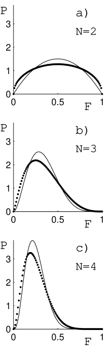
These probability distributions are presented in Fig. 2 together with exemplary numerical results. The behavior for $K\to\infty$ may be obtained by a saddle-point calculation, which we start from the form

$$P_{2,K}(F)=C(K)[F(1-F)]^{2(K-1)}\ {1\over 2}\int_{0}^{\infty}{dx\over x}\ [x+{1\over x}+2(1-2F)]^{2(1-K)}$$ (42)

using the symmetry of the integral with respect to the inversion $x\to 1/x$. We find as asymptotic form for $K\to\infty$

$$P_{2,K}(F)={\Gamma(2K+1/2)\over\Gamma(3/2)\Gamma(2K-1)}\ F^{2(K-1)}\ \sqrt{1-F}\ \bigl{[}1+\ O\bigl{(}\frac{1}{K}\bigr{)}\bigr{]}\ .$$ (43)

As expected, for large dimensionality $K$ this distribution tends to a delta function located at $\langle F\rangle$, which in the limit $K\to\infty$ tends to unity according to (34).

Figure 2: Probability distribution of fidelity for random one–qubit states generated according to the induced measures $\mu_{2,K}$ where $K=1$ ($\triangle$), $K=2$ ($\square$), and $K=3$ ($\Diamond$) $K=4$ ($\circ$). Flat distribution represents averaging over pure states, while full symbols refer to the Hilbert–Schmidt measure, $K=N=2$. Solid lines represent Eq. (15) and (37), while dashed line denotes the case $K=3/2$ corresponding to the Bures distribution (40).

V.3 General case, $N\geq 3$, average values

In the general case one has to use the general formula for fidelity, (4), not as convenient for analytical computations as Eq. (7) valid for $N=2$. Before describing the analytical results let us compare the problem for an arbitrary $N$ with the symmetric case, in which the averaging in both arguments is performed over the set of pure states. For any nonsingular measure covering the entire set of mixed states, the mean value will be larger than $1/N$, since the mean distance between random mixed states is smaller than the mean distance between random pure states.

This statement concerns in particular all induced measures $\mu_{N,K}$ analyzed for a fixed system size $N$. Since the mean purity decreases with the size $K$ of the ancilla, $\langle{\rm Tr}\rho^{2}\rangle=(N+K)/(NK+1)$ ZS01 , one may infer that $\langle F\rangle_{N,K}>\langle F\rangle_{N,L}$ if $K>L$. In the analogy to the simplest case $N=2$ one may thus expect that for any $N$ the mean fidelity tends to unity, $\lim_{K\to\infty}\langle F\rangle_{N,K}=1$.

Veracity of this reasoning may be checked by analysis of the following general results, derived in the Appendix A for an arbitrary induced measure $\mu_{N,K}$. We are going to study the moments of the root fidelity $\langle\sqrt{F}\rangle_{N,K}$, so the second moment gives the average fidelity. Let us denote $n=K-N\geq 0$ and introduce constants

$$G(m)=\Bigl{(}\frac{\Gamma(KN)}{\Gamma(KN+m/2)}\Bigr{)}^{2}\ .$$ (44)

Defining an auxiliary matrix of size $N$

$$(X_{n})_{k,l}:=\Gamma(n+k+l-1)\Gamma(n+l){\rm\quad for\quad}k,l=1,2,...,N.$$ (45)

the rather complicated averages may be written down in a concise way,

$$\langle\sqrt{F}\rangle_{N,K}=G(1)\ {\rm Tr}[X_{n}^{-1}X_{n+1/2}]$$ (46)

and

$$\langle F\rangle_{N,K}=G(2)\Bigl{[}{\rm Tr}\bigl{(}X_{n}^{-1}X_{n+1}\bigr{)}+\Bigl{(}{\rm Tr}\bigl{(}X_{n}^{-1}X_{n+1/2}\bigr{)}\Bigr{)}^{2}-{\rm Tr}\Bigl{(}\bigl{(}X_{n}^{-1}X_{n+1/2}\bigr{)}^{2}\Bigr{)}\Bigr{]}$$ (47)

The above formula is one of the main results of this paper. For $N=2$ one needs to work with matrices $X_{n}$ of size $2$. Computing the necessary traces one shows that (47) simplifies to formula (34), while (46) allows to write down an explicit formula

$$\langle\sqrt{F}\rangle_{2,K}=\Bigl{(}{\Gamma(2K)\over\Gamma(2K+\frac{1}{2})}\Bigl{)}^{2}\Bigl{[}\frac{3}{2}\Bigl{(}{\Gamma(K+\frac{1}{2})\over\Gamma(K)}\Bigr{)}^{2}+\frac{1}{2}\Bigl{(}{\Gamma(K-\frac{1}{2})\over\Gamma(K-1)}\Bigr{)}^{2}\Bigr{]}.$$ (48)

For large $K$ this average tends to unity. This result was derived for $K\geq N$, and it is ill defined, e.g for $K=1$. Interestingly, by an analytical continuation $K\to 1$ one obtains the correct result for averaging over the space of pure states, $\langle\sqrt{F}\rangle_{2,1}=2/3$ in agreement with the trivial integral $\int_{0}^{1}\sqrt{F}dF$ following from the uniform distribution (15) with $N=2$. For the Bures measure we have $\langle\sqrt{F}\rangle_{2,3/2}=2^{7}13/(3^{2}5^{2}\pi^{2})\approx 0.7493$, while the average for the HS measure ($K=2$) is larger, $\langle\sqrt{F}\rangle_{2,2}=2^{5}31/(5^{2}7^{2})\approx 0.8098$.

Figure 3: Mean fidelity averaged over both states distributed according to the induced measure $\mu_{N,K}$, as a function of the size $K$ of the ancilla for $N=2$ ($\triangle$), $N=3$ ($\square$), $N=4$ ($\Diamond$), $N=5$ ($\circ$) and $N=6$ ($\times$). Solid lines denote analytical results, Eq. (34) and (47). Full symbols represent averaging over the Hilbert-Schmidt measure, $K=N$.

Analogous results obtained for $N=3$ from (46) and (47) read

$$\langle\sqrt{F}\rangle_{3,K}=\Bigl{(}{\Gamma(3K)\over\Gamma(3K+\frac{1}{2})}\Bigr{)}^{2}\Bigl{[}\frac{3}{8}\Bigl{(}{\Gamma(K-\frac{3}{2})\over\Gamma(K-2)}\Bigr{)}^{2}+\frac{3}{4}\Bigl{(}{\Gamma(K-\frac{1}{2})\over\Gamma(K-1)}\Bigr{)}^{2}+\frac{15}{8}\Bigl{(}{\Gamma(K+\frac{1}{2})\over\Gamma(K)}\Bigr{)}^{2}\Bigr{]}$$ (49)

and

$$\langle F\rangle_{3,K}=\frac{1}{3}+\frac{1}{K^{2}}\Bigl{[}\Bigl{(}{\Gamma(K-\frac{1}{2})\over\Gamma(K-1)}\Bigr{)}^{2}\Bigl{[}\frac{5}{12}\Bigl{(}{\Gamma(K+\frac{1}{2})\over\Gamma(K)}\Bigr{)}^{2}+\frac{1}{12}\Bigl{(}{\Gamma(K-\frac{3}{2})\over\Gamma(K-2)}\Bigr{)}^{2}\Bigr{]}+\frac{1}{6}\Bigl{(}\frac{\Gamma(K+\frac{1}{2})\Gamma(K-\frac{3}{2})}{\Gamma(K)\Gamma(K-2)}\Bigr{)}^{2}\Bigr{]}.$$ (50)

In the limit $K\to\infty$ both results tend to unity, e.g. $\langle F\rangle_{3,K}\to\frac{1}{3}+\frac{5}{12}+\frac{1}{12}+\frac{1}{6}=1$. As in the case $N=2$, the above formulae hold for $K\geq N$, but by analytical continuation for $K\to 1$ one obtains correct results for averaging over the space of for pure states $\langle\sqrt{F}\rangle_{3,1}=8/15$ and $\langle F\rangle_{3,1}=1/3$. Also results in the limit $K\to 2$, $\langle F\rangle_{3,2}=1/3+15(\pi/32)^{2}\approx 0.4779$ agree with the data obtained numerically by averaging over the manifold of the mixed states with rank $K=2$. Numerical results obtained from a sample of $10^{6}$ random states, presented in Fig. 3, confer with predictions obtained by means of the general formula (47). Interestingly, the mean fidelity for the HS measure, $K=N$, decreases with the system size $N$.

V.4 General case, $N\geq 3$, probability distributions

Figure 3 presents the distributions of fidelity $P_{N,K}(F)$, averaged symmetrically over both states distributed according to the induced measures $\mu_{N,K}$ for $N=2,3$ and $4$. Analytical results (15) available for pure states ($K=1$) are marked by solid lines. In general, the larger size $K$ of the ancilla, the more the distribution is shifted toward higher values of $F$, since both states get closer to the maximally mixed state. For large size of the ancilla the distributions become concentrated at the mean value $\langle F\rangle_{N,K}$ which tends to unity in the limit $K\to\infty$.

Figure 4: Probability distribution of fidelity while averaging symmetrically over both states distributed according to induced measures $\mu_{N,K}$. The size of the system equals a) $N=3$ and b) $N=4$ and while the size $K$ of the ancilla is coded by symbols: $K=1$ ($\triangle$), $K=2$ ($\square$), $K=3$ ($\Diamond$) and $K=4$ ($\circ$). Full symbols represent averaging over Hilbert–Schmidt measure, $K=N$. Solid line for $K=1$ denote Eq. (15), dotted lines are plotted to guide the eye.

Obtaining explicitly analytical results for the probability distribution $P_{N,K}(F)$ in the general case of arbitrary $N$ and $K$ seems not to be simple. However, we may obtain required information concerning these distributions by studying the sequence of higher momenta of the root fidelity. Knowing all moments $\langle(\sqrt{F})^{m}\rangle_{N,K}$ for $m=2,4,...$ we may in principle extract the desired distribution $P_{N,K}(F)$. To compute such moments for $K\geq N$ we construct a generating function

$$Z(\lambda)=\det\Bigl{(}\sum_{m=0}^{\infty}\frac{(-\lambda)^{m}}{m!}\Gamma\bigl{(}\frac{m}{2}+k+l+K-N-1\bigr{)}\Gamma\bigl{(}\frac{m}{2}+l+K-N\bigr{)}\Bigr{)}$$ (51)

which we obtain by replacing the fixed trace ensembles for $\rho_{1}$ and $\rho_{2}$ by Laguerre ensembles and integrating out eigenvectors of $\sqrt{\rho_{1}}\rho_{2}\sqrt{\rho_{1}}$ with the help of the Itzykson–Zuber integral. The determinant concerns a $N\times N$ matrix with indices, $k,l=1,..,N$. To obtain the mean values of $(\sqrt{F})^{m}$ one needs to multiply the expansion coefficients of $Z(\lambda)$ by constants $G(m)$ defined in (44):

$$\langle(\sqrt{F})^{m}\rangle_{N,K}=G(m)\ (-d/d\lambda)^{m}\ Z(\lambda)/Z(0)|_{\lambda=0}$$ (52)

For any fixed $N$ the moments are analytic in $K$, so one may try to use the analytic extension for the cases $K<N$. Alternatively, we may treat this case separately, investigating another generating function

$$Z_{K}(\lambda)=\det\Bigl{(}\sum_{m=0}^{\infty}\frac{(-\lambda)^{m}}{m!}\bigl{[}\Gamma\bigl{(}\frac{m}{2}+k+N-K\bigr{)}\bigr{]}^{2}\ \frac{\Gamma\bigl{(}\frac{m}{2}+k+l-1\bigr{)}}{\Gamma\bigl{(}\frac{m}{2}+k+l+N-2K\bigr{)}}\Bigr{)}$$ (53)

with determinant of a $K\times K$ matrix with indices, $k,l=1,..,K$. This formula holds for $N\geq 2K$, but may be extended analytically in $N$ beyond this restriction. It is obtained by reducing $\sqrt{\rho_{1}}\rho_{2}\sqrt{\rho_{1}}$ by unitary rotations to the spaces of nonzero eigenvalues with dimension $K\leq N$ using the symmetry properties of the fidelity and again integrating out all unitary rotations with the help of the Itzykson–Zuber integral, (here applied two times).

To show an application of this approach let us expand the generating function $Z_{K}$ up to the second order in $\lambda$. Fixing $K=2$ we obtain the averages for variable $N$

$$\langle\sqrt{F}\rangle_{N,2}=\frac{\sqrt{\pi}}{16}\ (22N-13)\ \Bigl{(}\frac{\Gamma(2N)}{\Gamma\bigr{(}2N+\frac{1}{2}\bigl{)}}\Bigr{)}^{2}\ \frac{\Gamma\bigl{(}N-\frac{1}{2}\bigr{)}}{\Gamma(N)}$$ (54)

and

$$\langle F\rangle_{N,2}=\frac{1}{N}\Bigl{[}1+\frac{3\pi}{16}\ \frac{\Gamma\bigr{(}N-\frac{1}{2}\bigl{)}\Gamma\bigr{(}N+\frac{1}{2}\bigl{)}}{\Gamma(N-1)\Gamma(N+1)}\Bigr{]}$$ (55)

These formulae are valid for arbitrary $N$, and for $N=2,3$ are consistent with Eqs. (48)- (50). In a similar way one may proceed with $K=3,4...$. Furthermore, expanding the generating function to the $m$-th order one could calculate the expectation values of $(\sqrt{F})^{m}$ and obtain further information concerning the probability distribution $P_{N,K}(F)$. There are analogous formulas for the moments $\langle(\sqrt{F})^{m}\rangle_{N,K}$ to Eqs. (46), (47) in terms of traces involving $K\times K$ matrices.

To give an explicit expression for the distribution of fidelity $P_{N,K}(F)=W(\sqrt{F})/2\sqrt{F}$ we start from the fixed trace ensemble with traces $t_{1}={\rm Tr}\rho_{1}$, $t_{2}={\rm Tr}\rho_{2}$, $t_{3}={\rm Tr}(\sqrt{\rho_{1}}\rho_{2}\sqrt{\rho_{1}})^{1/2}$. We take the Laplace transform with respect to $t_{1},t_{2},t_{3}$, calculate it and then apply the inverse Laplace transform at $t_{1}=1$, $t_{2}=1$, and $t_{3}=\sqrt{F}$. What we obtain is a threefold contour integral

$$W(\sqrt{F})=C\int{ds_{1}{\rm e}^{s_{1}}\over 2\pi i{s_{1}}^{KN}}\ \int{ds_{2}{\rm e}^{s_{2}}\over 2\pi i{s_{2}}^{KN}}\ \int{ds_{3}{\rm e}^{\sqrt{F}s_{3}}\over 2\pi i}\ Z({s_{3}\over\sqrt{s_{1}s_{2}}})\ .$$ (56)

with $C=\Gamma(K^{2}N^{2})/Z(0)$. It is easy to see, that this equation is equivalent to Eq. (52). All three contours go along the whole imaginary axis with a small positive real part. We need the analytic properties of the function $Z(x)$ which can be seen from the form

$$Z(x)=\det\left(2\int_{0}^{\infty}dy{y^{k-2}\Gamma[k-1+2(K-N+l)]\over(y+1/y+x)^{k-1+2(K-N+l)}}\right)\ .$$ (57)

$Z(x)$ has a cut along the real axis for $x\leq-2$ and behaves asymptotically for $x\to\infty$ like $(\ln x)^{N}/x^{2KN}$, which is not easy to see, but can be derived from an explicit form for $Z(x)$

$$Z(x)=\det\bigl{[}(d/dx)^{2(K-N+l-1)+k}H_{k}(x)\ln(x/2+\sqrt{x^{2}/4-1})\bigr{]}$$ (58)

with

$$H_{k}(x)=-{\Bigl{[}\bigl{(}x/2+\sqrt{x^{2}/4-1}\bigr{)}^{k-1}+\bigl{(}x/2-\sqrt{x^{2}/4-1}\bigr{)}^{k-1}\Bigr{]}}/\sqrt{x^{2}/4-1}$$ (59)

For later use we need also for $x>2$ (in the following $\epsilon>0$)

$$\lim_{\epsilon\to 0}\bigl{[}Z(-x-i\epsilon)\bigr{]}=\det\bigl{[}(d/dx)^{2(K-N+l-1)+k}H_{k}(x)\ln\bigl{(}x/2+\sqrt{x^{2}/4-1}\bigr{)}+i\pi(d/dx)^{2(K-N+l-1)+k}H_{k}(x)\bigr{]}\ .$$ (60)

Using appropriate contour deformations and partial integrations we are able to perform the $s_{1}$ and $s_{2}$ integrations arriving at:

$$W(\sqrt{F})=\frac{\Gamma(K^{2}N^{2})}{Z(0)\pi^{2}}\lim_{\epsilon\to 0}\Bigl{[}\int_{2}^{\infty}dxB(x){\rm Im}[Z(-x-i\epsilon)]\Bigr{]}$$ (61)

with

$$B(x)=F^{KN-1}\int_{2}^{2/\sqrt{F}}{dy\over\sqrt{1-Fy^{2}/4}}{\theta(x-y)\ (x-y)^{2KN-3}\over(2KN-3)!}\ .$$ (62)

Finally for numerical convenience we may use the following integral representations for $x>2$: $Z(x)=\det(A_{1})$ and $\lim_{\epsilon\to 0}[Z(-x-i\epsilon)]=\det(A_{1}-iA_{2})$ with

$$A_{1}=4\int_{0}^{\infty}{du\cosh[(k-1)u]\Gamma[k-1+2(K-N+l)]\over[2\cosh(u)+x]^{k-1+2(K-N+l)}}$$ (63)

and

$$A_{2}=4\int_{0}^{\pi}{du\cos[(k-1)u]\Gamma[k-1+2(K-N+l)]\over[2\cos(u)+x]^{k-1+2(K-N+l)}},$$ (64)

where $k,l=1,\dots,N$, so $A_{1}$ and $A_{2}$ are square matrices of size $N$.

VI Concluding remarks

In this work we have posed and solved the problem of computing the average fidelity between two random quantum states. As easy to predict, the results depend heavily on the probability measure, according to which the quantum states are generated. We have concentrated on two cases, we consider to be the most important: the Bures measure $\mu_{\rm B}$, used to guess a random state of size $N$ in lack of any other information, and the induced measure $\mu_{N,K}$, applied if it is known that the mixed state is obtained by partial trace over a $K$ dimensional environment. The latter case reduces to the Hilbert-Schmidt measure if $K=N$.

In general, one has to distinguish the case of the symmetric averaging, in which both states are generated according to the same measure, and the asymmetric case, e.g. the problem of computing the mean fidelity between a pure random state and a mixed random state.

In particular we have obtained explicit results for symmetric averaging over the induced measures $\mu_{N,K}$, which have a simple physical interpretation. The mean value $\langle F\rangle_{N,K}$ corresponds to the case of picking at random pure states in $N\times K$ dimensional Hilbert space and then studying the fidelity between both mixed states obtained by partial tracing over the $K$–dimensional environment.

In certain cases we have derived the probability distribution for fidelity $P(F)$ which may be used to formulate statistical statements which evaluate quantitatively certain quantum operations and quantum protocols. For instance, the universal protocol of quantum cloning of a $N$ dimensional pure state gives the fidelity $F_{u}=(N+3)/(2N+2)$ We98 . Making use of the distribution (15) we see that the probability $p_{N}$ that a randomly taken $N$ dimensional pure state will give a better fidelity than this obtained by the cloning procedure is equal

$$p_{N}=\int_{F_{u}}^{1}P_{N,1}(F)dF=\frac{1}{2^{N-1}}\ \Bigl{(}\frac{N-1}{N+1}\Bigr{)}^{N-1}.$$ (65)

For $N=2$ there exists a considerable probability, $p_{2}=1/6$, that picking at random a pure state of a qubit provides results better then the cloning protocol. However, for larger system sizes the probability $p_{N}$ decreases exponentially with $N$, which means that the relative strength of the cloning procedure with respect to the ’random choice’ strategy, increases with the size of the system.

We thank D. Savin for useful discussions and I. Bengtsson, R. Muǹoz-Tapia and A. Uhlmann for helpful correspondence. This work was supported by Sonderforschungsbereich / Transregio 12 der Deutschen Forschungsgemeinschaft and a solicitated grant number PBZ-MIN-008/P03/2003 of Polish Committee for Scientific Research.

Appendix A Generating functions for moments

A.1 Induced measures: Wishart case, $K\geq N$

In this appendix we present a brief derivation of the generating functions for moments of the square-root fidelity which hold for an arbitrary induced measure $\mu_{N,K}$. In the first subsection we consider the case $K\geq N$. Then the distribution of square-root fidelity is given by

$$W(\sqrt{F})\propto\int D\rho_{1}\ \int D\rho_{2}\ \det(\rho_{1}\rho_{2})^{K-N}\delta(1-{\rm Tr}\rho_{1})\ \delta(1-{\rm Tr}\rho_{2})\ \delta\Bigl{(}\sqrt{F}-{\rm Tr}\bigl{(}\sqrt{\rho_{1}}\rho_{2}\sqrt{\rho_{1}}\bigr{)}^{1/2}\Bigr{)},$$ (66)

where $D\rho_{1}$, $D\rho_{2}$ are the matrix volume elements and we have to integrate over positive matrices $\rho_{1}$ and $\rho_{2}$. Since ${\rm Tr}((\sqrt{\rho_{1}}\rho_{2}\sqrt{\rho_{1}})^{1/2})$ is a homogeneous function of both, $\rho_{1}$ and $\rho_{2}$ of degree $1/2$, moments can equivalently be obtained from the generating function

$$Z(\lambda)\propto\int D\rho_{1}\ \int D\rho_{2}\ \det(\rho_{1}\rho_{2})^{K-N}{\rm e}^{-{\rm Tr}\rho_{1}}\ {\rm e}^{-{\rm Tr}\rho_{2}}\ {\rm e}^{-\lambda{\rm Tr}[(\sqrt{\rho_{1}}\rho_{2}\sqrt{\rho_{1}})^{1/2}]}$$ (67)

following Equ. (52). We make a transformation $\rho_{2}$ $\to$ ${\rho_{1}}^{-1/2}\rho_{2}{\rho_{1}}^{-1/2}$ and taking into account the Jacobian we obtain

$$Z(\lambda)\propto\int D\rho_{1}\ \int D\rho_{2}\ \det(\rho_{1})^{-N}\det(\rho_{2})^{K-N}{\rm e}^{-{\rm Tr}\rho_{1}}\ {\rm e}^{-{\rm Tr}\rho_{2}/\rho_{1}}\ {\rm e}^{-\lambda{\rm Tr}(\rho_{2})^{1/2}}\ .$$ (68)

Note that the nasty square roots disappeared and we can use the Itzykson–Zuber integral to integrate out the eigenvectors of $\rho_{2}$ in the expression ${\rm e}^{-{\rm Tr}\rho_{2}/\rho_{1}}$. As result we obtain

$$Z(\lambda)\propto\int_{0}^{\infty}{dx_{1}\over x_{1}}...{dx_{N}\over x_{N}}\int dy_{1}...dy_{N}(y_{1}...y_{N})^{K-N}{\rm e}^{-(x_{1}+...x_{N})}\ {\rm e}^{-\lambda(\sqrt{y_{1}}+...\sqrt{y_{N}})}\ \det({\rm e}^{-y_{k}/x_{l}})\prod_{k<l}(x_{k}-x_{l})(y_{k}-y_{l})\$$ (69)

where $x_{1},...x_{N}$ are the eigenvalues of $\rho_{1}$ and $y_{1},...y_{N}$ are the eigenvalues of $\rho_{2}$. Using the properties of the Vandermonde determinant we reduce this expression to a single determinant and arrive at Eq. (57).

A.2 Induced measures: anti–Wishart case, $K<N$

In this case the matrices $\rho_{1}$ and $\rho_{2}$ are of rank $K$ and they can be brought by a unitary transformation of the form

$$U=\left(\begin{matrix}\sqrt{1-XX^{\dagger}}&-X\cr X^{\dagger}&\sqrt{1-X^{\dagger}X}\cr\end{matrix}\right)$$

to block diagonal form. If $U$ is drawn from CUE it can be shown that the corresponding measure $DX$ is flat, where $X$ is a complex $K\times(N-K)$ matrix with the restriction $XX^{\dagger}\leq 1$. Calling the nonzero blocks again $\rho_{1}$ and $\rho_{2}$, now $K\times K$ matrices, we may write the generating function for moments as

$$Z_{K}(\lambda)\propto\int D\rho_{1}\ \int D\rho_{2}\ \int_{XX^{\dagger}\leq 1}DX\ \det(\rho_{1}\rho_{2})^{N-K}{\rm e}^{-{\rm Tr}\rho_{1}}\ {\rm e}^{-{\rm Tr}\rho_{2}}\ {\rm e}^{-\lambda{\rm Tr}[(\sqrt{\rho_{1}}\sqrt{1-XX^{\dagger}}\rho_{2}\sqrt{1-XX^{\dagger}}\sqrt{\rho_{1}})^{1/2}]}\ .$$ (70)

In a first step we make the transformation $\rho_{2}$ $\to$ $(1-XX^{\dagger})^{-1/2}\rho_{2}(1-XX^{\dagger})^{-1/2}$ arriving at

$$Z_{K}(\lambda)\propto\int D\rho_{1}\ \int D\rho_{2}\ \int_{XX^{\dagger}\leq 1}DX\ {\det(\rho_{1}\rho_{2})^{N-K}\over\det(1-XX^{\dagger})^{N}}{\rm e}^{-{\rm Tr}\rho_{1}}\ {\rm e}^{-{\rm Tr}\rho_{2}/(1-XX^{\dagger})}\ {\rm e}^{-\lambda{\rm Tr}[(\sqrt{\rho_{1}}\rho_{2}\sqrt{\rho_{1}})^{1/2}]}\ .$$ (71)

Then we use the symmetry ${\rm Tr}((\sqrt{\rho_{1}}\rho_{2}\sqrt{\rho_{1}})^{1/2})={\rm Tr}((\sqrt{\rho_{2}}\rho_{1}\sqrt{\rho_{2}})^{1/2})$ and make the transformation $\rho_{1}$ $\to$ ${\rho_{2}}^{-1/2}\rho_{1}{\rho_{2}}^{-1/2}$ leading to

$$Z_{K}(\lambda)\propto\int D\rho_{1}\ \int D\rho_{2}\ \int_{XX^{\dagger}\leq 1}DX\ {\det(\rho_{1})^{N-K}\over\det(\rho_{2})^{K}\det(1-XX^{\dagger})^{N}}{\rm e}^{-{\rm Tr}\rho_{1}/\rho_{2}}\ {\rm e}^{-{\rm Tr}\rho_{2}/(1-XX^{\dagger})}\ {\rm e}^{-\lambda{\rm Tr}\sqrt{\rho_{1}}}\ .$$ (72)

Now we see that the matrix $W=XX^{\dagger}$ is again of the Wishart type and is positive definite for $K\leq(N-K)$. Let us focus on this case, then the distribution of $W$ is $\propto\det(W^{N-2K})$ and we may reduce the integral to the eigenvalues $x_{1},...x_{K}$ of $\rho_{1}$, $y_{1},...y_{K}$ of $\rho_{2}$ and ${z_{1},...z_{K}}$ of $W$ using two times the Itzykson–Zuber integral. The resulting expression contains in the integrand the Vandermonde determinants of $x_{1},...x_{K}$ and of $z_{1},...z_{K}$ and can therefore again be reduced to a single determinant which is given by

$$Z_{K}(\lambda)=\det\left(2\int_{0}^{\infty}dx\int_{0}^{\infty}{dy\over y}\int_{0}^{1}dz{x^{N-K+k-1}z^{N-2K}\over(1-z)^{N-K-l+1}}\exp\left[-\sqrt{{x\over 1-z}}\left(y+{1\over y}\right)\right]{\rm e}^{-\lambda\sqrt{x}}\right)\ .$$ (73)

Expanding the threefold integral in powers of $\lambda$, one arrives at Eq. (53).

Appendix B Derivation of the distribution (21)

To derive the distribution $P(F)$ for the fidelity between a random pure state and a random mixed state distributed according to the Bures measure (10) consider

$$P({F})\propto\int_{\rho>0}D\rho\ \int_{A=A^{\dagger}}DA\ \delta(1-{\rm Tr}\rho A^{2})\ \delta(1-{\rm Tr}\rho)\ \delta({F}-{\rm Tr}\rho|\psi\rangle\langle\psi|),$$ (74)

where we introduced an auxiliary Hermitian matrix $A$ to generate the distribution (10) and the last two $\delta$-functions correspond to the constraints (1) and (13). The $\delta$-functions may be written as inverse Laplace transforms along the slightly to the right shifted imaginary axis and then the integration over the positive definite $N\times N$-matrix $\rho$ can be done arriving at

$$P({F})\propto\int{ds_{1}{\rm e}^{s_{1}}\over 2\pi i}\ \int{ds_{2}{\rm e}^{s_{2}}\over 2\pi i}\ \int{ds_{3}{\rm e}^{{F}s_{3}}\over 2\pi i}\ \int DA\det(s_{1}A^{2}+s_{2}+s_{3}|\psi\rangle\langle\psi|)^{-N}\ .$$ (75)

After a suitable rescaling of the matrix A, we can do the $s_{1}$- and $s_{3}$-integrations and obtain

$$P({F})\propto\int{DA\over\det(1+A^{2})^{N}}\int_{-i\infty+\epsilon}^{+i\infty+\epsilon}{ds{\rm e}^{s}\over 2\pi is^{N^{2}/2-N}}\ (\langle\psi|(1+A^{2})^{-1}|\psi\rangle)^{-N}\ F^{N-1}\ \exp\Bigl{(}-{sF\over\langle\psi|(1+A^{2})^{-1}|\psi\rangle}\Bigr{)}\ .$$ (76)

Now it is possible to show, that with the correspondence $U=(1+iA)/(1-iA)$ the measure $DA/\det(1+A^{2})^{N}$ is equivalent to the invariant measure on the group of unitary $N\times N$-matrices $U$. Since only $\langle\psi|(1+A^{2})^{-1}|\psi\rangle=\langle\psi|(2+U+U^{\dagger})/4|\psi\rangle$ occurs, the integration over $A$ can be reduced to a one-dimensional one and after integrating over $s$ in the complex plane and restoring the normalization we end up with formula (21).

References

• (1) D. J. C. Bures, Trans. Am. Math. Soc. 135, 199 (1969).
• (2) R. Jozsa, J. Mod. Opt. 41 2315, (1994).
• (3) A. Uhlmann, Rep. Math. Phys. 9, 273 (1976).
• (4) V. Bužek and M. Hillery, Phys. Rev. A 54, 1844 (1996).
• (5) N. J. Cerf, Phys. Rev. Lett. 84, 4497 (2000)
• (6) T. Prosen, Phys. Rev. E 65, 036208 (2002).
• (7) M. D. Bowdrey, D. K. L. Oi, A. J. Short, K. Banaszek and J. A. Jones, Phys. Lett. A 294, 258 (2002).
• (8) M. A. Nielsen, Phys. Lett. A 303, 249 (2002).
• (9) E. Bagan, M. Baig, and R. Muñoz–Tapia Phys. Rev. A 67, 014303 (2003).
• (10) M. J. Hall, Phys. Lett. A 242, 123 (1998).
• (11) K. Życzkowski and H.-J. Sommers, J. Phys. A 34, 7111 (2001).
• (12) H.-J. Sommers and K. Życzkowski, J. Phys. A 37, 8457 (2004).
• (13) D. Petz and C. Sudár, J. Math. Phys. 37, 2662 (1996)
• (14) M. A. Nielsen and I. L. Chuang, Quantum Computation and Quantum Information, Cambridge University Press, Cambridge, 2000.
• (15) A. Uhlmann, Phys. Lett. A 161, 329 (1992).
• (16) A. Uhlmann, Rep. Math. Phys. 36, 461 (1995).
• (17) M. Hübner, Phys. Lett. A 163, 239 (1992).
• (18) P. B. Slater, J. Phys. A 32, 8231 (1999).
• (19) H.–J. Sommers and K. Życzkowski, J. Phys. A 36, 10083 (2003).
• (20) E. Lubkin, J. Math. Phys. 19, 1028 (1978).
• (21) S. Lloyd and H. Pagels, Ann. Phys. (N.Y.), 188, 186 (1988).
• (22) D. Page, Phys. Rev. Lett. 71, 1291 (1993).
• (23) Y.-K. Yu and Y.-C. Zhang Physica A 312, 1 (2002)
• (24) R. A. Janik and M. A. Nowak J.Phys. A 36, 3629 (2003)
• (25) M. Kuś, J. Mostowski and F. Haake J. Phys. A 21, L1073 (1988).
• (26) K. Życzkowski and H.-J. Sommers, J. Phys. A 33, 2045 (2000).
• (27) E. Bagan, M. Baig, R. Muñoz–Taipa and A. Rodriguez, Phys. Rev. A 69, 010304 (2004).
• (28) R. Werner, Phys. Rev. A 58, 1827 (1998).