Quantum Error Correction on Linear Nearest Neighbor Qubit Arrays

Abstract

A minimal depth quantum circuit implementing 5-qubit quantum error correction in a manner optimized for a linear nearest neighbor architecture is described. The canonical decomposition is used to construct fast and simple gates that incorporate the necessary swap operations. Simulations of the circuit’s performance when subjected to discrete and continuous errors are presented. The relationship between the error rate of a physical qubit and that of a logical qubit is investigated with emphasis on determining the concatenated error correction threshold.

The field of quantum computation deals with the manipulation of 2-state quantum systems called qubits. Many different physical systems are being investigated in the race to build a scalable quantum computer Kane (1998); Engel et al. (2001); Giovannetti et al. (2000); Hinds (2001); James (2000); Mooij (1999). Due to the fragility of quantum systems, one property a scalable architecture must possess is the ability to implement quantum error correction (QEC) Shor (1995); Laflamme et al. (1996); Niwa et al. (2002). The question has been raised as to how well QEC can be implemented on a linear nearest neighbor (LNN) quantum computer Gottesman (2000) due to the expectation that numerous swap gates will be required. Working out a way around this is important due to the large number of LNN architectures currently under investigation Wu et al. (1999); Vrijen et al. (2000); Golding and Dykman (2003); Novais and Neto (2003); Hollenberg et al. (2003); Tian and Zoller (2003); Yang et al. (2003); Feng et al. (2003); Pachos and Knight (2003); Friesen et al. (2003); Vandersypen et al. (2002); Solinas et al. (2003); Jefferson et al. (2002); Petrosyan and Kurizki (2002); Golovach and Loss (2002); Ladd et al. (2002); V’yurkov and Gorelik (2000); Kamenetskii and Voskoboynikov (2003). In this paper a 5-qubit QEC circuit appropriate for an LNN architecture is presented that is as efficient as the best known circuit for an architecture able to interact arbitrary pairs of qubits Braunstein and Smolin (1997).

The paper is organized as follows. Firstly, the canonical decomposition used to construct efficient 2-qubit gates is discussed in brief. Details of the method used can be found in Kraus and Cirac . The Kane architecture Kane (1998) has been used to construct explicit decompositions, but the methods described apply to any architecture. The 5-qubit QEC scheme is then discussed and the LNN circuit presented. Following this, simulations of quantum data storage with and without QEC are presented. The paper concludes with a summary of all results.

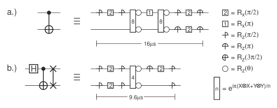
The canonical decomposition enables any 2-qubit operator $U_{AB}$ to be expressed (non-uniquely) in the form $V_{A}^{{\dagger}}\otimes V_{B}^{{\dagger}}U_{d}U_{A}\otimes U_{B}$ where $U_{A}$, $U_{B}$, $V_{A}$ and $V_{B}$ are single qubit unitaries and $U_{d}=\exp[i(\alpha_{x}X\otimes X+\alpha_{y}Y\otimes Y+\alpha_{z}Z\otimes Z)]$ Kraus and Cirac . Moreover, any entangling interaction can be used to create an arbitrary $U_{d}$ up to single qubit rotations Bremner et al. (2002). These two facts allow the construction of very efficient composite gates on any physical architecture. Fig. 1a shows the form of such a decomposed controlled-NOT (CNOT) on a Kane quantum computer Hill and Goan (2003); Kane (1998). The 2-qubit interaction corresponds to $\alpha_{x}=\alpha_{y}=\pi/8$, and $\alpha_{z}=0$. Z-rotations have been represented by quarter, half and three-quarter circles corresponding to $R_{z}(\pi/2)$, $R_{z}(\pi)$, and $R_{z}(3\pi/2)$ respectively. Full circles represent Z-rotations of angle dependent on the physical construction of the computer. Square gates 1 and 2 correspond to X-rotations $R_{x}(\pi)$ and $R_{x}(\pi/2)$. Fig. 1b shows an implementation of the composite gate Hadamard followed by CNOT followed by swap (HCNOTS). Note that the total time of the compound gate is significantly less than the CNOT on its own.

Figure 1: Decomposition into physical operations of a.) CNOT gate b.) Hadamard, CNOT then swap. Note that the Kane architecture has been used for illustrative purposes. In addition to the clear speed advantage when implementing compound gates, the decomposed CNOT gate is faster than its adiabatic equivalent (26$\mu$s) Fowler et al. (2003)

The implication of the above is that the swaps inevitably required in an LNN architecture to bring qubits together to be interacted can be incorporated into other gates without additional cost. Indeed, in certain cases LNN circuits built out of compound gates are actually faster. With careful planning, general quantum circuits can be implemented on an LNN architecture with asymptotically the same number of gates as that required on an architecture that allows any pair of qubits to be interacted.

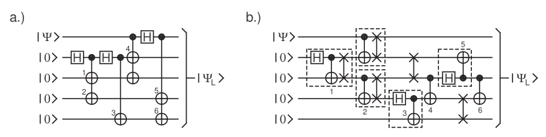
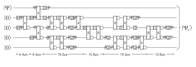
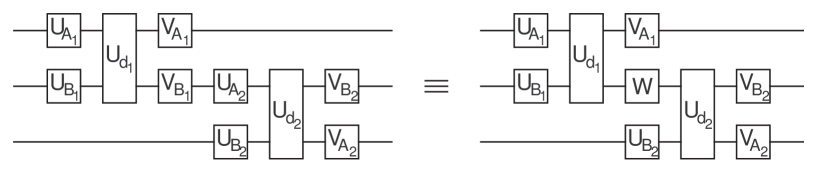
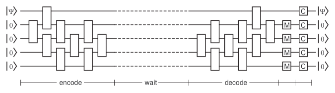
5-qubit quantum error correction schemes are designed to correct a single arbitrary error. No single error correction scheme can use less than 5 qubits Nielson and Chuang (2000). A number of 5-qubit QEC proposals exist Braunstein and Smolin (1997); Knill et al. (2001); Laflamme et al. (1996); Niwa et al. (2002); Bennett et al. (1996). Fig. 2b shows a circuit optimized for an LNN architecture implementing the encode stage of the QEC scheme proposed in Braunstein and Smolin (1997). For reference, the original circuit is shown in fig. 2a. Note that the LNN circuit uses exactly the same number of CNOTs and achieves minimal depth. The two extra swaps required do not significantly add to the total time of the circuit. Fig. 3 shows an equivalent physical circuit for a Kane quantum computer. Note that this circuit uses the fact that if two 2-qubit gates share a qubit then two single-qubit unitaries can be combined as shown in fig. 4. The decode circuit is simply the encode circuit run backwards. All 5-qubit QEC schemes are only useful for data storage Niwa et al. (2002) due to the difficulty of interacting two logical qubits. Fig. 5 shows a full encode-wait-decode-measure-correct data storage cycle. Table 1 shows the range of possible measurements and the action required in each case.

Figure 2: a.) 5-qubit encoding circuit for general architecture b.) equivalent circuit for linear nearest neighbor architecture with dashed boxes indicating compound gates. CNOT gates that must be performed sequentially are numbered.

Figure 3: A sequence of physical gates implementing the circuit of fig. 2b. Note the Kane architecture has been used for illustrative purposes.

Figure 4: Circuit equivalence used to reduce the number of physical gates in fig. 3.

Figure 5: A complete encode-wait-decode-measure-correct QEC cycle.

Measurement	Action
$\Psi^{\prime}\otimes$0000	I$\otimes$IIII
$\Psi^{\prime}\otimes$0001	I$\otimes$IIIX
$\Psi^{\prime}\otimes$0010	Z$\otimes$IIXI
$\Psi^{\prime}\otimes$0011	I$\otimes$IIXX
$\Psi^{\prime}\otimes$0100	I$\otimes$IXII
$\Psi^{\prime}\otimes$0101	X$\otimes$IXIX
$\Psi^{\prime}\otimes$0110	Z$\otimes$IXXI
$\Psi^{\prime}\otimes$0111	X$\otimes$IXXX
$\Psi^{\prime}\otimes$1000	Z$\otimes$XIII
$\Psi^{\prime}\otimes$1001	I$\otimes$XIIX
$\Psi^{\prime}\otimes$1010	X$\otimes$XIXI
$\Psi^{\prime}\otimes$1011	X$\otimes$XIXX
$\Psi^{\prime}\otimes$1100	Z$\otimes$XXII
$\Psi^{\prime}\otimes$1101	X$\otimes$XXIX
$\Psi^{\prime}\otimes$1110	XZ$\otimes$XXXI
$\Psi^{\prime}\otimes$1111	Z$\otimes$XXXX

Table 1: Action required to correct the data qubit $\Psi^{\prime}$ vs measured value of ancilla qubits. Note that the X-operations simply reset the ancilla.

When simulating the QEC cycle, the circuit of fig. 2b was used to keep the analysis architecture independent. Each gate was modelled as taking the same time, allowing the time $T$ to be made an integer such that each gate takes one time step. Gates were furthermore simulated as though perfectly reliable and errors applied to each qubit (including idle qubits) at the end of each time step. The rationale for including idle qubits is that in an LNN architecture physical manipulation of some description is required to decouple neighboring qubits which inevitably leads to errors.

Two error models were used — discrete and continuous. In the discrete model a qubit can suffer either a bit-flip (X), phase-flip (Z) or both simultaneously (XZ). Each type of error is equally likely with total probability of error $p$ per qubit per time step. The continuous error model involves applying single-qubit unitary operations of the form

$$U_{\sigma}=\left(\begin{array}[]{cc}\cos(\theta/2)e^{i(\alpha+\beta)/2}&\sin(\theta/2)e^{i(\alpha-\beta)/2}\\ -\sin(\theta/2)e^{i(-\alpha+\beta)/2}&\cos(\theta/2)e^{i(-\alpha-\beta)/2}\end{array}\right)$$ (1)

where $\alpha$, $\beta$, and $\theta$ are normally distributed about 0 with standard deviation $\sigma$.

Both the single qubit and single logical qubit (5 qubits) systems were simulated. The initial state

$$|\Psi\rangle=\frac{5}{13}|0\rangle+\frac{12}{13}|1\rangle$$ (2)

was used in both cases as $|\langle\Psi|X|\Psi\rangle|^{2}\cong 0.5$, $|\langle\Psi|Z|\Psi\rangle|^{2}\cong 0.5$, and $|\langle\Psi|XZ|\Psi\rangle|^{2}=0$ thus allowing each type of error to be detected. Simpler states such as $|0\rangle$, $|1\rangle$, $(|0\rangle+|1\rangle)/\sqrt{2}$, and $(|0\rangle-|1\rangle)/\sqrt{2}$ do not have this property. For example, the states $|0\rangle$ and $|1\rangle$ are insensitive to phase errors, whereas the other two states are insensitive to bit flip errors. Let $T_{wait}$ denote the duration of the wait stage. Note that the total duration of the encode, decode, measure and correct stages is 14. In the QEC case the total time $T=T_{wait}+14$ of one QEC cycle was varied to determine the time that minimizes the error per time step defined by

$$\epsilon_{step}=1-\sqrt[T]{1-\epsilon_{final}}$$ (3)

where $\epsilon_{final}=1-|\langle\Psi^{\prime}|\Psi\rangle|^{2}$ and $|\Psi^{\prime}\rangle$ is the final logical qubit state. An optimal time $T_{opt}$ exists since the logical qubit is only protected during the wait stage and the correction process can only cope with one error. If the wait time is zero, extra complexity has been added but no corrective ability. Similarly, if the wait time is very large, it is almost certain that more than one error will occur, resulting in the qubit being destroyed during the correction process. Somewhere between these two extremes is a wait time that minimizes $\epsilon_{step}$. Table 2 shows $T_{opt}$, $\epsilon_{step}$ and the reduction in error $\epsilon_{step}/p$ versus $p$ for discrete errors. Table 3 shows the corresponding data for continuous errors. Note that, in the continuous case, the single qubit $p$ has been obtained via 1-qubit simulations and a 1-qubit version of equation 3.

$p$	$T_{opt}$	$\epsilon_{step}$	$\epsilon_{step}/p$
$10^{-2}$	25	$1.7\times 10^{-2}$	$1.7\times 10^{0}$
$1.6\times 10^{-3}$	40	$1.6\times 10^{-3}$	$1.0\times 10^{0}$
$10^{-3}$	50	$8.4\times 10^{-4}$	$8.4\times 10^{-1}$
$10^{-4}$	150	$3.1\times 10^{-5}$	$3.1\times 10^{-1}$
$10^{-5}$	750	$1.1\times 10^{-6}$	$1.1\times 10^{-1}$
$10^{-6}$	1500	$3.2\times 10^{-8}$	$3.2\times 10^{-2}$
$10^{-7}$	6000	$1.1\times 10^{-9}$	$1.1\times 10^{-2}$
$10^{-8}$	10000	$2.0\times 10^{-11}$	$2.0\times 10^{-3}$

Table 2: Probability per time step $\epsilon_{step}$ of a discrete error when using 5-qubit QEC vs physical probability $p$ per qubit per time step of a discrete error.

$\sigma$	$T_{opt}$	$p$	$\epsilon_{step}$	$\epsilon_{step}/p$
$10^{-1}$	$2.5\times 10^{1}$	$5.9\times 10^{-2}$	$6.9\times 10^{-3}$	$1.2\times 10^{-1}$
$10^{-2}$	$2.5\times 10^{2}$	$5.9\times 10^{-3}$	$1.4\times 10^{-5}$	$2.4\times 10^{-3}$
$10^{-3}$	$2.5\times 10^{3}$	$6.0\times 10^{-4}$	$1.3\times 10^{-8}$	$2.2\times 10^{-5}$
$10^{-4}$	$2.5\times 10^{4}$	$6.0\times 10^{-5}$	$1.0\times 10^{-11}$	$1.7\times 10^{-7}$
$10^{-5}$	$2.5\times 10^{5}$	$6.0\times 10^{-6}$	$7.2\times 10^{-15}$	$1.2\times 10^{-9}$

Table 3: Probability per time step $\epsilon_{step}$ of a discrete error when using 5-qubit QEC vs standard deviation $\sigma$ of continuous errors.

An enormous range of threshold error rates $p$ exist in the literature. These start at a very pessimistic $p=10^{-8}$ Knill et al. (1996) and go up to a very optimistic $p=2\times 10^{-3}$ Zalka (1996). The first thing that can be noted from the discrete simulation data of Table 2 is that the LNN threshold $p=1.6\times 10^{-3}$ is comparable to the most optimistic previous estimate which was made using 7-qubit fault tolerant QEC with errors applied only after gate operations and not to idle qubits. The error rate $p=1.6\times 10^{-3}$ should not however be thought of as the allowable operating error rate of a physical quantum computer as precisely no improvement in error rate is achieved when using QEC. If an error rate improvement of a factor of 10 or 100 is desired when using QEC then $p=10^{-5}$ or $p=10^{-7}$ is required respectively. Further work is required to determine the error rate improvement required to allow robust implementation of large scale quantum algorithms with a reasonable number of error correction qubits.

For continuous errors, there is no true threshold. Even for very large random unitary rotations an improvement is still gained by using the LNN QEC circuit. In this case, provided gates can be implemented such that the angles associated with the continuous error model are of order $10^{-2}$, an improvement in error rate of at least a factor of 100 can be achieved.

Further work is required to determine whether the discrete or continuous error model or some other model best describes errors in physical quantum computers.

In conclusion, we have presented an efficient circuit for 5-qubit QEC on an LNN architecture and simulated its effectiveness against both discrete and continuous errors. It was found that, for the discrete error model, if error correction is to provide an error rate reduction of a factor of 10 or 100, the physical error rate $p$ must be $10^{-5}$ or $10^{-7}$ respectively. For the continuous error model, it was acceptable for error angles to have a standard deviation of up to $10^{-2}$ radians as using QEC still gives an error rate improvement better than a factor of 100.

Further simulation is required to determine the error thresholds associated with 1- and 2-qubit LNN error-corrected gates.

References

- Kane (1998) B. E. Kane, Nature 393, 133 (1998).
- Engel et al. (2001) H.-A. Engel et al., Solid State Commun. 119, 229 (2001).
- Giovannetti et al. (2000) V. Giovannetti et al., J. Mod. Optic. 47, 2187 (2000).
- Hinds (2001) E. Hinds, Phys. World pp. 39–43 (2001).
- James (2000) D. F. V. James, Fortschr. Physik 48, 823 (2000).
- Mooij (1999) J. E. Mooij, Microelectron. Eng. 47, 3 (1999).
- Shor (1995) P. W. Shor, Phys. Rev. A 52, R2493 (1995).
- Laflamme et al. (1996) R. Laflamme et al., Phys. Rev. Lett. 77, 198 (1996).
- Niwa et al. (2002) J. Niwa et al., quant-ph/0211071 (2002).
- Gottesman (2000) D. Gottesman, J. Mod. Optic. 47, 333 (2000).
- Wu et al. (1999) N.-J. Wu et al., quant-ph/9912036 (1999).
- Vrijen et al. (2000) R. Vrijen et al., Phys. Rev. A 62, 012306 (2000).
- Golding and Dykman (2003) B. Golding and M. I. Dykman, cond-mat/0309147 (2003).
- Novais and Neto (2003) E. Novais and A. H. C. Neto, cond-mat/0308475 (2003).
- Hollenberg et al. (2003) L. C. L. Hollenberg et al., cond-mat/0306235 (2003).
- Tian and Zoller (2003) L. Tian and P. Zoller, quant-ph/0306085 (2003).
- Yang et al. (2003) K. Yang et al., Chinese Phys. Lett. 20, 991 (2003).
- Feng et al. (2003) M. Feng et al., quant-ph/0304169 (2003).
- Pachos and Knight (2003) J. K. Pachos and P. L. Knight, Phys. Rev. Lett. 91, 107902 (2003).
- Friesen et al. (2003) M. Friesen et al., Phys. Rev. B 67 (2003).
- Vandersypen et al. (2002) L. M. K. Vandersypen et al., quant-ph/0207059 (2002).
- Solinas et al. (2003) P. Solinas et al., Phys. Rev. B 67 (2003).
- Jefferson et al. (2002) J. H. Jefferson et al., Phys. Rev. A 66 (2002).
- Petrosyan and Kurizki (2002) D. Petrosyan and G. Kurizki, Phys. Rev. Lett. 89, 207902 (2002).
- Golovach and Loss (2002) V. N. Golovach and D. Loss, Semicond. Sci. Tech. 17, 355 (2002).
- Ladd et al. (2002) T. D. Ladd et al., Phys. Rev. Lett. 89, 017901 (2002).
- V’yurkov and Gorelik (2000) V. V’yurkov and L. Y. Gorelik, quant-ph/0009099 (2000).
- Kamenetskii and Voskoboynikov (2003) E. O. Kamenetskii and O. Voskoboynikov, cond-mat/0310558 (2003).
- Braunstein and Smolin (1997) S. L. Braunstein and J. A. Smolin, Phys. Rev. A 55, 945 (1997).
- (30) B. Kraus and J. I. Cirac, Phys. Rev. A 63, 062309 (????).
- Bremner et al. (2002) M. J. Bremner et al., Phys. Rev. Lett. 89, 247902 (2002).
- Hill and Goan (2003) C. D. Hill and H.-S. Goan, Phys. Rev. A 68 (2003).
- Fowler et al. (2003) A. G. Fowler et al., Phys. Rev. A 67, 012301 (2003).
- Nielson and Chuang (2000) M. A. Nielson and I. L. Chuang, Quantum Computation and Quantum Information (Cambridge University Press, Cambridge, 2000).
- Knill et al. (2001) E. Knill et al., Phys. Rev. Lett. 86, 5811 (2001).
- Bennett et al. (1996) C. H. Bennett et al., Phys. Rev. A 54, 3824 (1996).
- Knill et al. (1996) E. Knill et al., quant-ph/9610011 (1996).
- Zalka (1996) C. Zalka, quant-ph/9612028 (1996).