Quantum Feedback Control of Atomic Motion in an Optical Cavity LA-UR-03-6826

Abstract

We study quantum feedback cooling of atomic motion in an optical cavity. We design a feedback algorithm that can cool the atom to the ground state of the optical potential with high efficiency despite the nonlinear nature of this problem. An important ingredient is a simplified state-estimation algorithm, necessary for a real-time implementation of the feedback loop. We also describe the critical role of parity dynamics in the cooling process and present a simple theory that predicts the achievable steady-state atomic energies.

The control of quantum systems is a problem that lies at the heart of several fields, including atom optics and nanomechanics. Many of the techniques developed thus far for controlling quantum systems in an initially unknown state involve the use of dissipative processes to achieve a well-defined final state, as in the laser cooling methods in atom optics Metcalf99 . A different paradigm for cooling involves modifying the system Hamiltonian based on information provided by measurements (i.e., quantum feedback control). Such a strategy for control is generally applicable to quantum as well as classical systems Raizen98 ; Belavkin99 ; Doherty00 ; Armen02 ; Vitali03 ; Hopkins03 ; Geremia03 . As quantum-limited measurement techniques become more available, quantum feedback control is likely to soon be an essential element in atom-optical and nanomechanical toolkits.

One of the most promising avenues for the study of quantum feedback control centers on experiments in cavity quantum electrodynamics (CQED), where a single quantum system may be monitored continuously in real time, as has been demonstrated in a series of pioneering experiments Hood98 ; Mabuchi99 ; Hood00 ; Pinkse00 . Furthermore, the optical potential due to the cavity light provides an easily adjustable means for applying forces on the atom. Feedback has been shown to increase the storage time for atoms in such an experimental system Fischer02 . Despite these efforts, however, CQED feedback cooling has not yet been conclusively demonstrated, highlighting the need for a deeper theoretical understanding of this system as well as more sophisticated, higher performance cooling algorithms. Our goal here is to develop approximate estimation and control algorithms for cooling the atomic motion in such a CQED system—an “active cooling” approach that is distinct from passive cavity cooling methods Horak97 . We will then analyze the performance of these algorithms both analytically and through numerical simulations. This problem is particularly interesting due to the nonlinear form of the measurement operator, a situation distinct from previous studies of nonlinear quantum feedback control Doherty00 ; Wiseman02 . An important issue that we address here is whether the (Gaussian) estimation methods developed for linear systems are still effective in this problem.

The setup we are considering is an atom in a microcavity in the strong-coupling regime, as in the aforementioned CQED experiments Hood98 ; Mabuchi99 ; Hood00 ; Pinkse00 , but where the output light is monitored via homodyne detection Wiseman93 , which gives information about the atomic position in the cavity Quadt95 . We consider the case where the light is resonant with the cavity, but the detuning from atomic resonance is much larger than the natural atomic linewidth. We thus analyze the coupled atom-cavity system after adiabatic elimination of the cavity and internal atomic dynamics Doherty98 . The resulting stochastic master equation (SME) in Itô form Kloeden92 for the atomic motion conditioned on the homodyne measurement, describing the observer’s best estimate for the atomic state, is

$$\begin{array}[]{rcl}d\rho&{}={}&\displaystyle-i[H_{\mathrm{eff}},\rho]\,dt-\Gamma[\cos^{2}(\tilde{k}X),[\cos^{2}(\tilde{k}X),\rho]]\,dt\\ &&\displaystyle-\sqrt{2\eta\Gamma}\{[\cos^{2}(\tilde{k}X),\rho]_{+}-2\langle\cos^{2}(\tilde{k}X)\rangle\rho\}\,dW.\end{array}$$ (1)

The effective atomic Hamiltonian is

$$H_{\mathrm{eff}}=\pi P^{2}-{V_{\mathrm{max}}}\cos^{2}(\tilde{k}X),$$ (2)

and $dW$ is given in terms of the scaled photodetector current (measurement record) $d\tilde{r}$ by

$$dW=d\tilde{r}(t)/\sqrt{\eta}+\sqrt{8\eta\Gamma}\langle\cos^{2}(\tilde{k}X)\rangle dt.$$ (3)

The physical interpretation of Eqs. (1) and (3) is that the photocurrent is a direct measurement of $\cos^{2}(\tilde{k}X)$ within the adiabatic approximation. In these expressions, we are using scaled units such that position is measured in units of $\sqrt{\hbar/(m\omega_{\mathrm{\scriptscriptstyle HO}})}$, momentum is measured in units of $\sqrt{\hbar m\omega_{\mathrm{\scriptscriptstyle HO}}}$, and time is measured in units of $2\pi/\omega_{\mathrm{\scriptscriptstyle HO}}$, where $\omega_{\mathrm{\scriptscriptstyle HO}}:=\alpha gk\sqrt{2\hbar/|m\Delta|}$ is the oscillation frequency in the harmonic approximation for one of the optical potential wells, $g$ is the CQED coupling constant, $m$ is the atomic mass, $\Delta$ is the detuning from the atomic resonance, $\eta$ is the photodetection efficiency, $\alpha$ is the mean cavity photon number in the absence of the atom, $k$ is the optical spatial frequency, $\tilde{k}:=k\sqrt{\hbar/(m\omega_{\mathrm{\scriptscriptstyle HO}})}$, ${V_{\mathrm{max}}}:=\pi/\tilde{k}^{2}$, $\Gamma:={2\alpha^{2}g^{4}}/{(\Delta^{2}\kappa\omega_{\mathrm{\scriptscriptstyle HO}})}$ is the effective measurement strength, $\kappa$ is the energy decay rate of the cavity, and $dr(t)=\sqrt{\kappa/\omega_{\mathrm{\scriptscriptstyle HO}}}\,d\tilde{r}(t)$ is the physical photocurrent. The model thus has only three independent parameters, $\tilde{k}$, $\Gamma$, and $\eta$, in addition to any parameters that specify how the optical potential is modulated. For the atomic parameters, we consider cesium driven on the D₂ line, so that $m=2.21\times 10^{-25}\;\mathrm{kg}$ and $k=11732\;\mathrm{cm}^{-1}$. For the cavity parameters, we choose values similar to those used in recent CQED experiments Hood98 ; Mabuchi99 ; Hood00 , yielding $\kappa/2\pi=40$ MHz, $g/2\pi=120$ MHz, and $\alpha=1$. We also assume an optical detuning of $\Delta/2\pi=4\;\mathrm{GHz}$ to the red of the atomic resonance. The corresponding scaled parameters are $\Gamma=23.6$ and $\tilde{k}=0.155$. The scaled depth of the optical potential is ${V_{\mathrm{max}}}=131$, so that the lowest two band energies are within 1% of their values in the harmonic approximation. We also choose the idealized detection efficiency of $\eta=1$. However, cooling performance similar to that shown below is achievable even in the presence of detector inefficiency ($\eta$ well below $0.5$) as well as other real-world limitations such as hardware propagation and computation delays inprep .

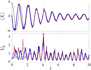
Figure 1: Tracking behavior of the Gaussian estimator for the position centroid and variance for a sample trajectory. The expectation values for the true wave packet (heavy lines) are shown with the corresponding Gaussian estimator quantities (narrow lines). The cooling algorithm was activated at $t=2$.

While integration of the SME in order to obtain a state estimate is sensible in principle, in practice it is much too difficult to integrate the SME in real time. To solve this problem we must simplify the estimator. We make a Gaussian ansatz for the atomic Wigner function (which, equivalently, prescribes how the Weyl-ordered moments of the atomic state factorize). In doing so, we reduce the effort of integrating a partial differential equation to the much more manageable effort of integrating a set of five coupled ordinary differential equations for the two means $\langle X\rangle$ and $\langle P\rangle$ and the three variances $V_{x}$, $V_{p}$, and $C_{xp}:=\langle XP+PX\rangle-\langle X\rangle\langle P\rangle$ EPAPS . The tracking behavior of the Gaussian estimator is illustrated in Fig. 1, which compares the evolution of the position mean and variance for an atom evolving according to Eq. (1) with the same quantities from a Gaussian estimator evolution beginning with a different initial condition. The estimator rapidly locks on to the true solution. The ability of the estimator to track both quantities well is crucial to the success of the control algorithm that we present here.

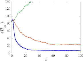
Figure 2: Evolution of the mean effective energy $\langle H_{\mathrm{eff}}\rangle$ (relative to the minimum potential energy), illustrating the cooling-algorithm performance. Shown are: cooling via the Gaussian estimator (heavy solid), cooling based on the photocurrent signal (narrow solid), and free atomic evolution with no cooling (dashed). Each curve is an average of 128 trajectories.

Intuitively, an algorithm that responds to the wave-packet centroid, raising the optical potential while the atom is climbing one side of a well, should cool the atom. However, such a strategy eventually breaks down due to uncontrolled pumping of energy into the wave-packet variances. The key to obtaining an effective control algorithm is to consider the energy evolution due to the Hamiltonian part of the SME: $\partial_{t}\langle{H}_{\mathrm{eff}}\rangle_{\mathrm{fb}}=-(\partial_{t}{V_{\mathrm{max}}})\langle\cos^{2}(\tilde{k}X)\rangle$. From this expression, it is clear that a “bang-bang” strategy is optimal for cooling if we consider only cyclic modulations of the potential amplitude within a limited range. The potential should be switched to the extreme low value when the quantity $-\langle\cos^{2}(\tilde{k}X)\rangle$ is maximized and to the extreme high value when this quantity is minimized. We denote these extreme values of the potential by $(1-\varepsilon)^{2}{V_{\mathrm{max}}}$ and $(1+\varepsilon)^{2}{V_{\mathrm{max}}}$. Such a control strategy is sensitive to energy in both the centroids and variances of the atom. Of course, it is not possible to tell whether $-\langle\cos^{2}(\tilde{k}X)\rangle$ is at an extremum based only on information at the current time. Thus, to complete the feedback algorithm, we fit a quadratic curve to the history of this quantity at each time step and trigger on the slope of this curve at the current time.

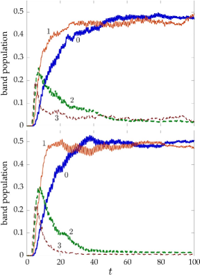
Figure 3: Evolution of the band populations for the lowest four energy bands of the optical lattice, averaged over 128 trajectories. Top: cooling based on the Gaussian estimator. Bottom: cooling based on perfect knowledge of the actual wave function.

An example of the cooling algorithm in action is shown in Fig. 2, which compares the energy evolution for an ensemble of atoms (where each atom is cooled separately in an independent simulation) undergoing cooling for $\varepsilon=0.1$ with the energy evolution without any cooling (i.e., free evolution in the optical potential). Without cooling, the atoms simply heat up due to the measurement back-action (or equivalently, the stochastic cavity decay process), until they are eventually lost from the optical potential. The heating rate is set by the second term in the SME: $\partial_{t}\langle{H}_{\mathrm{eff}}\rangle_{\mathrm{meas}}=8\pi\Gamma\langle\cos^{2}(\tilde{k}X)\sin^{2}(\tilde{k}X)\rangle$. The cooling algorithm is able to counteract the measurement heating, and the atoms settle to a steady-state energy much lower than the initial energy. Also shown in Fig. 2 is the cooling performance of a much simpler algorithm, which arises by noting that the photocurrent is a direct measure of $-\langle\cos^{2}(\tilde{k}X)\rangle$ (plus noise), and that it should be possible to cool the atoms by triggering on the photocurrent signal itself (an approach similar in spirit to the “differentiating feedback” strategy in Ref. Fischer02 ). In this case, the same quadratic curve-fitting procedure is used to temper the measurement noise. Although cooling to a steady state still occurs in this case, the cooling performance is substantially worse than for the Gaussian estimator. This indicates that the Gaussian estimator acts as a nearly optimal filter (in the same sense as a Kalman filter Doherty99 ) for the relevant information in the photodetector signal. The results shown were generated assuming initial conditions and curve-fit details as follows, although the results do not sensitively depend on these values: The atoms begin in a coherent state ($V_{x}=V_{p}=1/2$), and each has an initial centroid energy corresponding to a displacement from the well center of 58% of the distance to the edge of the well, chosen so the atoms are clearly trapped but not particularly cold. The initial locations of the atoms are distributed uniformly between the bottom of the well and this maximum distance. The Gaussian estimator begins with the (impure-state) initial conditions $\langle X\rangle_{\mathrm{e}}=6$, $\langle P\rangle_{\mathrm{e}}=0$, ${V_{X}^{\mathrm{e}}}={V_{P}^{\mathrm{e}}}=1/\sqrt{2}$, and $C_{\mathrm{e}}=0$. The estimator is evolved in steps of $\Delta t=0.0005$, and at each step the quadratic curve is fitted to the values of $-\langle\cos^{2}(\tilde{k}X)\rangle$ computed from the 300 most recent estimator steps.

The cooling performance is further illustrated in Fig. 3, which shows the populations in the lowest four bands of the optical potential. Most of the steady-state population is in the lowest two bands, accounting for 94% of the population, and these two bands are almost equally populated. We now show that this behavior can be understood in terms of the parity of the atomic state. The atomic parity is invariant under Hamiltonian evolution in the atomic potential (and hence the influence of the control algorithm). However, the measurement term in the SME causes the atomic parity to diffuse according to

$$d\langle\mathcal{P}\rangle=-\sqrt{8\eta\Gamma}\left[\langle\mathcal{P}\cos(2\tilde{k}X)\rangle-\langle\mathcal{P}\rangle\langle\cos(2\tilde{k}X)\rangle\right]\,dW,$$ (4)

where $\mathcal{P}$ is the parity operator. In fact, this is an unbiased, nonstationary diffusion process that causes $\langle\mathcal{P}\rangle$ to “purify” at late times to the extreme values $\pm 1$ of pure parity, so that the homodyne measurement acts like a QND measurement of the atomic parity. Since the atomic initial condition described above corresponds to $\langle\mathcal{P}\rangle=0$, the measurement process drives the atoms to states with either pure even or pure odd parity with equal probability. The obvious consequence of this effect for cooling is that only half of the atoms can be cooled to the ground band, while the remaining half can be cooled at best to the first excited band EPAPS . However, due to this purification effect (which means that the observer knows the final state of the atom on each individual run), cooling to the first excited band is essentially equivalent to cooling to the ground state, since the atom can be driven between these two bands with an additional coherent process (e.g., modulation via an additional classical optical potential).

Much of the residual energy (excitation out of the lowest two bands) is due to the inability of the Gaussian estimator to perfectly track the true atomic state. In this light, the cooling performance is quite impressive, especially considering the highly non-Gaussian nature of the first excited state, toward which half the atoms are cooling. To show this behavior explicitly, we can remove the estimator from the problem, and repeat the same ensemble of simulations where the cooling algorithm operates based on the value of $-\langle\cos^{2}(\tilde{k}X)\rangle$ computed with respect to the actual atomic wave function. These results are also shown in Fig. 3, and in this case the lowest two bands account for 98% of the atomic population.

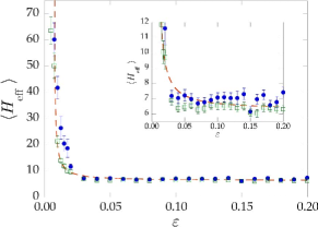
Figure 4: Final energies, measured over the interval from $t=90$ to $100$, as the switching amplitude $\varepsilon$ varies. Circles: cooling based on the Gaussian estimator. Squares: cooling based on perfect knowledge of the actual wave function. Dashed line: simple cooling theory, Eq. (5). Inset: magnified view of the same data. Error bars reflect standard errors from averages over 128 trajectories.

The steady-state atomic energies can be well described by a simple analytic theory, which we now derive. We will assume that the atomic energy is near the ground-state energy $E_{0}$, so that we can make the harmonic approximation for the potential. We will further assume for the moment that all the energy $\Delta E$ in excess of $E_{0}$ is associated with the wave-packet centroid (i.e., the wave packet is not squeezed). Then the quantity $-{V_{\mathrm{max}}}\langle\cos^{2}(\tilde{k}X)\rangle$ exhibits oscillations of peak-to-peak magnitude $\Delta E$. Assuming that the switching occurs at the extremal times, the energy-evolution expression above leads to a coarse-grained cooling rate of $\partial_{t}\langle{H}_{\mathrm{eff}}\rangle_{\mathrm{fb}}=-8\varepsilon(\langle{H}_{\mathrm{eff}}\rangle-E_{0})$. On the other hand, the heating rate discussed above can be rewritten as $\partial_{t}\langle{H}_{\mathrm{eff}}\rangle_{\mathrm{meas}}=4\Gamma\tilde{k}^{4}\langle{H}_{\mathrm{eff}}\rangle$. Steady state occurs when these two rates sum to zero:

$$\langle{H}_{\mathrm{eff}}\rangle_{\mathrm{ss}}=\frac{E_{0}+E_{1}}{2(1-\beta)}.$$ (5)

Here, $\beta:=\Gamma\tilde{k}^{4}/2\varepsilon$, and we have made the replacement $E_{0}\rightarrow(E_{0}+E_{1})/2$ in view of the above parity considerations, where $E_{1}$ is the energy of the first excited band.

We can also derive a theory for the other extreme, where we assume all the excess energy is associated purely with squeezing of the wave packet and not with the centroid. In this case, the oscillations of $-{V_{\mathrm{max}}}\langle\cos^{2}(\tilde{k}X)\rangle$ are of peak-to-peak magnitude $\sqrt{\langle H_{\mathrm{eff}}\rangle^{2}-E_{0}^{2}}$. Then the $(1-\beta)^{-1}$ dependence in Eq. (5) is replaced by $(1-\beta^{2})^{-1/2}$. In the regime $\beta\ll 1$ where this theory should be valid, this prediction is always below that of Eq. (5), and thus the centroid-only theory more faithfully represents the physical cooling limit.

Eq. (5) is compared with simulated late-time energies in Fig. 4. The simulated energies are in good agreement with the simple theory, although they are generally higher than the simple theoretical prediction. Again, much of this discrepancy is due to the imperfect tracking behavior of the Gaussian estimator, and the simulated energies from cooling based on perfect knowledge of the actual wave function are in better agreement. Qualitatively, we see a transition between ineffective and effective cooling with $\varepsilon$; essentially, $\varepsilon$ must be large enough that the cooling rate exceeds the heating rate, ensuring that the system is controllable. Beyond this transition, the system displays a remarkable insensitivity to the value of the switching amplitude; we observe similar robustness to the changes in the other parameters $\Gamma$, $\tilde{k}$, and $\eta$.

The authors would like to thank Andrew Doherty and Sze Tan for helpful discussions. This research was performed in part using the resources of the Advanced Computing Laboratory, Institutional Computing Initiative, and LDRD program of Los Alamos National Laboratory.

References

- (1) H. J. Metcalf and P. van der Straten, Laser Cooling and Trapping (Springer, New York, 1999).
- (2) M. G. Raizen et al., Phys. Rev. A58, 4757 (1998).
- (3) V. P. Belavkin, Rep. Math. Phys., 43, 405 (1999).
- (4) A. C. Doherty et al., Phys. Rev. A62, 012105 (2000).
- (5) M. A. Armen et al., Phys. Rev. Lett. 89, 133602 (2002).
- (6) D. Vitali, S. Mancini, L. Ribichini, and P. Tombesi, J. Opt. Soc. Am. B20, 1054 (2003).
- (7) A. Hopkins, K. Jacobs, S. Habib, and K. Schwab, Phys. Rev. B80, 235328 (2003).
- (8) JM Geremia, J. K. Stockton, and H. Mabuchi, arXiv.org preprint quant-ph/0309034.
- (9) C. J. Hood, M. S. Chapman, T. W. Lynn, and H. J. Kimble, Phys. Rev. Lett. 80, 4157 (1998).
- (10) H. Mabuchi, J. Ye, and H. J. Kimble, Appl. Phys. B 68, 1095 (1999).
- (11) C. J. Hood et al., Science 287, 1447 (2000).
- (12) P. W. H. Pinkse, T. Fischer, P. Maunz, and G. Rempe, Nature (London) 404, 365 (2000).
- (13) T. Fischer et al., Phys. Rev. Lett. 88, 163002 (2002).
- (14) P. Horak et al., Phys. Rev. Lett. 79, 4974 (1997).
- (15) H. M. Wiseman, S. Mancini, and J. Wang, Phys. Rev. A66, 013807 (2002).
- (16) H. M. Wiseman and G. J. Milburn, Phys. Rev. A47, 642 (1993).
- (17) R. Quadt, M. Collett, and D. F. Walls, Phys. Rev. Lett. 74, 351 (1995).
- (18) A. C. Doherty, A. S. Parkins, S. M. Tan, and D. F. Walls, Phys. Rev. A57, 4804 (1998).
- (19) P. E. Kloeden and E. Platen, Numerical Solution of Stochastic Differential Equations (Springer, Berlin, 1992).
- (20) D. A. Steck et al., in preparation.
- (21) See EPAPS Document No. E-PRLTAO-92-053419 for sample animations of two quantum trajectories and details regarding the Gaussian estimator. A direct link to this document may be found in the online reference section for this article at http://link.aps.org/abstract/PRL/v92/e223004.
- (22) A. C. Doherty and K. Jacobs, Phys. Rev. A60, 2700 (1999).