A quantitative model for the effective decoherence
of a quantum computer with imperfect unitary operations

Abstract

The problem of the quantitative degradation of the performance of a quantum computer due to noisy unitary gates (imperfect external control) is studied. It is shown that quite general conclusions on the evolution of the fidelity can be reached by using the conjecture that the set of states visited by a quantum algorithm can be replaced by the uniform (Haar) ensemble. These general results are tested numerically against quantum computer simulations of two particular periodically driven quantum systems.

I Introduction

In the last decade quite a few studies have been carried on which focus on the behaviour of an imperfect quantum computer (q.c.) Nielsen and Chuang (2000). Although the sources of imperfections are in general specific to each particular physical implementation, they can be grouped in two categories Preskill (1998), decoherence and unitary errors.

Decoherence consists in an unwanted interaction between the q.c. and the surrounding environment, due to imperfect isolation Zurek (2003). This coupling causes the two parties to become entangled, so that the state of the q.c. alone is no more described by a pure state but by a density matrix. Its consequences on the results of a computation, which prompted for the development of error correction strategies, have been studied from the very early days of quantum computing early_dec ; active corrections (error correction codes) are already sufficiently understood to be covered in standard textbooks (see Nielsen and Chuang, 2000, chapters 8-10), while passive methods (decoherence free subspaces) have been developed more recently (see Lidar and Whaley, 2003, for a review).

Even in a q.c. perfectly isolated from the environment the computation can still be affected by unitary errors; the state evolution remains coherent, but the algorithm is slightly modified. Unitary errors arise in at least two different contexts: they may be due to an imperfect implementation of the operations by means of which the computation is performed (noisy gates, n.g.) or to a residual Hamiltonian leading to an additional spurious evolution of the q.c. memory (static errors, s.e.).

The lack of knowledge about the parameters determining the unitary errors implies some level of uncertainty for the results of the computation, that is, unitary errors can be thought of as an effective decoherence mechanism. While true decoherence and n.g. are to a certain extent similar in their effects, s.e. differ because time correlations cannot be neglected. This is particularly clear, for instance, in ensemble computing, where the term incoherence is used Pravia et al. (2003): even if the action of s.e. is described by completely positive superoperators, it can be corrected by locally unitary “refocussing” operations.

The effects of imperfections can be summarised by means of a relation between an “imperfection intensity” $\epsilon$ and the timescale $t_{d}$ for the degradation of some characteristic quantity linked to the computational process. The usual choice Miquel et al. (1997) for this quantity is the fidelity, defined as the squared modulus of the overlap between the state $|\,\psi\,\rangle=U|\,\psi^{0}\,\rangle$ of the quantum memory after an ideal algorithm and the corresponding state $|\,\psi_{\ast}\,\rangle=U_{\ast}|\,\psi^{0}\,\rangle$ after an imperfect evolution of some type,

$$f=\left|\langle\,\psi\,|\,\psi_{\ast}\,\rangle\right|^{2}.$$ (1)

There is, recently, a rising interest in the problem of s.e, especially in connection to different signatures for integrable/chaotic dynamics static_err ; Benenti et al. (2001). The focus in this article will however be on n.g, which are less explored in the literature. The first investigations were based on simulations of Shor’s algorithm Shor (1997). In the seminal paper for the ion trap computer Cirac and Zoller (1995) the authors note that the quantum Fourier transform is quite robust with respect to an imperfect implementation of the laser pulses. A more systematic but still completely numerical analysis of the evolution of the fidelity in an almost identical setup was performed in Miquel et al. (1997). Although only Hadamard gates were considered to be noisy there, the empirical result captures the general behaviour $t_{d}\sim\epsilon^{-2}$.

Grover’s algorithm Grover (1997) was studied in Song and Kim (2003) with the help of a phenomenological model of probability diffusion, but the dependence of the model parameters on the number of qubits and $\epsilon$ was not determined. Conclusions similar to those in Miquel et al. (1997) were reached also in Shapira et al. (2003), where again the test algorithm was Grover’s one, and in a number of articles about the simulation of quantum chaotic maps Benenti et al. (2001); Song and Shepelyansky (2001); Chepelianskii and Shepelyansky (2002); Terraneo and Shepelyansky (2003); Levi et al. (2002). These results show that the timescale for the degradation of the fidelity of a q.c. decreases only polynomially with noise and system size.

The aim of this article is to perform a quantitative analysis of the effects of unbiased n.g. in a q.c. running a quantum algorithm without measurements (i.e. a multi-qubit unitary transformation). If $G$ is an elementary gate accessible to the q.c, its noisy implementation can be written as $G_{\ast}=\mathcal{E}G$, where $\mathcal{E}$ is a unitary error operator (in the following the symbol $\ast$ refers to the presence of imperfections); so, an ideal quantum algorithm is $U=\prod_{k}G_{k}$ and a noisy one is $U_{\ast}=\prod_{k}\mathcal{E}_{k}G_{k}$. The adjective “noisy” implies that there is no correlation for the error intensities of $\mathcal{E}_{k}$ and $\mathcal{E}_{k^{\prime}\neq k}$, and the adjective “unbiased” that for an error operator $\mathcal{E}=\mathbb{I}+O(\epsilon)$ the average over different realisations gives $\langle{\mathcal{E}}\rangle=\mathbb{I}+O(\epsilon^{2})$.

It will be shown that, in this “unitary model”, the degradation of the fidelity for n.g. depends only on the spectrum of the errors, on the size of the q.c. and on the number of gates in a given algorithm. Note that in an algorithm not involving measurements, the mean value of the fidelity is a directly measurable quantity; in fact, due to the previous considerations, it is sufficient to run the algorithm forward for $N_{g}/2$ gates, and then to apply the adjoint algorithm to go back to the initial state (which is known and which can be always chosen as an element of the computational basis). The average fidelity for $N_{g}$ gates is then exactly the probability of measuring this initial state, which can be done at each fixed precision with a fixed number of measurements.

The theoretical results are checked against numerical simulations based on two specific quantum algorithms calculating the evolution of a periodically driven quantum system (see appendix A), the sawtooth map Benenti et al. (2001) and the double-well map Chepelianskii and Shepelyansky (2002). The former is a purely unitary transformation, while the latter uses an ancilla and intermediate measurements. These numerical examples concern thus an imperfect q.c. used to simulate the evolution of another quantum system (with the q.c, in turn, simulated by a classical computer). Note that the choice of a particular set of primitive gates might affect the numerical checks but not the theoretical results, since the set is left unspecified there.

The proposed model and the numerical results suggest that a q.c. subject to a non-trivial computational task shows a sort of “universal” (algorithm-independent) behaviour for the fidelity degradation. The body of the article is organised as follows. Section II recalls the bounds to the fidelity degradation posed by the unitarity of errors. Section III introduces a detailed model for this degradation, whose predictions are tested numerically in section IV. The final part contains a discussion of open questions and limitations of this model. Various appendices explain the details of the calculations, of the implementation of quantum algorithms and of their numerical simulations.

II Fidelity degradation induced by unitary errors: a simple bound

As already said, a common approach in the study of unitary imperfections is to analyse their effects by means of the fidelity (equation 1), which can be seen as the probability of remaining on the state selected by the ideal algorithm. In a unitary error model a simple bound holds for its degradation; in fact, by introducing the squared norm of the difference of the state vectors one finds

$$\left\||\,\psi\,\rangle-|\,\psi_{\ast}\,\rangle\right\|^{2}=2(1-\Re\langle\,\psi\,|\,\psi_{\ast}\,\rangle)\geq 2(1-\sqrt{f}).$$

However, since $f$ does not depend on a global phase change on $|\,\psi_{\ast}\,\rangle$ (i.e. $U_{\ast}\rightarrow e^{i\chi}U_{\ast}$), while $\left\||\,\psi_{\ast}\,\rangle-|\,\psi\,\rangle\right\|$ does, one can take the minimum over $\chi$. In this case, the previous bound can be shown to become an equality:

$$\min_{\chi}\left\||\,\psi\,\rangle-e^{i\chi}|\,\psi_{\ast}\,\rangle\right\|^{2}=2(1-\sqrt{f}).$$ (2)

The squared norm can in turn be bounded by the norm of the operator implementing the algorithm. If the operator is diagonalisable this norm is of course the largest eigenvalue (in modulus). Introducing

$$\|A\|=\max_{|\,\phi\,\rangle}\|A|\,\phi\,\rangle\|,$$ (3)

which is normalised to $1$ for unitary operators, it is immediate to see from definition 3 that

$$\left\||\,\psi\,\rangle-e^{i\chi}|\,\psi_{\ast}\,\rangle\right\|\leq\left\|U-e^{i\chi}U_{\ast}\right\|.$$ (4)

The inequality $\|U_{1}U_{2}-W_{1}W_{2}\|\leq\|U_{1}-W_{1}\|+\|U_{2}-W_{2}\|$, which holds for unitary operators, implies that the majorisation chain can be continued with

$$\min_{\chi}\left\|U-e^{i\chi}U_{\ast}\right\| \leq \sum_{k}\min_{\chi_{k}}\left\|G_{k}-e^{i\chi_{k}}\mathcal{E}_{k}G_{k}\right\|$$

$$= \sum_{k}\min_{\chi_{k}}\left\|\mathbb{I}-e^{i\chi_{k}}\mathcal{E}_{k}\right\|\stackrel{{\scriptstyle def}}{{=}}\sum_{k}\varsigma_{\ast k},$$

where $\chi$ and the $\chi_{k}$’s are independent variables, since $\min_{\chi}\|\mathbb{I}-e^{i(\chi-\sum_{k}\chi_{k})}\|=0$. In this expression, the definition of $\varsigma_{\ast k}=\min_{\bar{\chi}}\left\|\mathbb{I}-e^{i\bar{\chi}}\mathcal{E}_{k}\right\|$ has been introduced. This quantity depends only on the spectrum of the error operator $\mathcal{E}_{k}$. This is easily shown by moving back to definition 3 and writing the generic vector $|\,\phi\,\rangle$ over an eigenbasis for $\mathcal{E}_{k}$; if the corresponding eigenvalues are $e^{i\lambda_{kj}}$ ($\lambda_{kj}\in\mathbb{R}$ since the errors are unitary), one obtains

$$\varsigma_{\ast k} = \min_{\chi}\max_{|\,\phi\,\rangle=\sum_{j}a_{kj}|\,\phi_{kj}\,\rangle}\left\|(\mathbb{I}-e^{i\chi}\mathcal{E}_{k})|\,\phi\,\rangle\right\|$$

$$= \min_{\chi}\max_{a_{kj}}\left\|{\textstyle\sum_{j}}a_{kj}(1-e^{i(\chi+\lambda_{kj})})|\,\phi_{kj}\,\rangle\right\|$$

$$= \min_{\chi}\max_{j}\left|1-e^{i(\chi+\lambda_{kj})}\right|=2\min_{\chi}\max_{j}\left|\;\sin\textstyle\frac{\chi+\lambda_{kj}}{2}\right|.$$

This already shows that only the eigenvalues $e^{i\lambda_{kj}}$ of $\mathcal{E}_{k}$ are relevant. Introducing finally the definition

$$\varsigma_{\ast}=\left\langle\varsigma_{\ast k}\right\rangle,$$ (6)

where the average for $\varsigma_{\ast}$ is on the type and the intensity of the errors, it is possible to conclude that

$$\min_{\chi}\left\|U-e^{i\chi}U_{\ast}\right\|^{2}\leq\Big{(}\sum_{k}\varsigma_{\ast k}\Big{)}^{2}=\varsigma_{\ast}^{2}N_{g}^{2}.$$ (7)

Therefore, using equation 2, 4 and 7, and multiplying by $1+\sqrt{f}\leq 2$, one obtains

$$1-f\leq\varsigma^{2}_{\ast}N^{2}_{g},$$ (8)

which shows that the degradation of the fidelity in a unitary error model cannot increase more than quadratically in the number of gates and in the error intensity. Of course, this result is only a majorisation, and the true average behaviour can be very different.

The quantity $\varsigma_{\ast}$ is in general algorithm dependent, because of the average over the type and the intensity of the errors, but only through the spectra of the error operators. In order to calculate $\varsigma_{\ast k}$, a non-trivial combined minimisation and maximisation is required. However, if $\mathcal{E}_{k}$ is assumed to be a small error, i.e. if all the angles $\lambda_{kj}$ are located in a narrow neighbourhood of radius $r_{k}$, it can be seen by geometric means that

$$\varsigma_{\ast k}=2\sin\frac{r_{k}}{2}\lesssim r_{k}.$$ (9)

III Fidelity degradation due to noisy gates: a perturbative model

The numerical simulations of the earlier articles about unitary errors, cited in the introduction, show that the degradation of the fidelity (definition 1) follows a law $f=\exp(-\alpha N_{g}\epsilon^{2})$, where $\epsilon$ expresses the “intensity” of the imperfections (see appendix C for the details about the error model underlying n.g.) and $\alpha$ is a parameter to be extracted with a fit. Since in this article the focus is on the small error limit, the goal is to find the value of $\alpha$ for $f\sim 1-\alpha N_{g}\epsilon^{2}$ (there are however arguments which support the extension to an exponential law). The generic limit in equation 8 can be specialised for the case of n.g. with the value $\varsigma_{\ast}=\epsilon/8$ (see formula 41):

$$1-f\leq\frac{N^{2}_{g}\epsilon^{2}}{64}.$$

As already said, the previous relation is only a majorisation. In particular, equation II takes into account the worst case scenario, where all the n.g. sum up coherently. One could conjecture that in a non-coherent scenario formula 7 should be modified by replacing $(\sum_{k}\varsigma_{\ast k})^{2}$ with $(\sum_{k}\varsigma_{\ast k}^{2})$, which reduces $N_{g}^{2}$ to $N_{g}$ (formula 42)

$$1-f\simeq\frac{N_{g}\epsilon^{2}}{48}.$$ (10)

As already said, exception made for the numerical coefficient, which is linked to the chosen error model, this result is completely general and can be found more simply by noting that each noisy gate transfers a probability of order $\epsilon^{2}$ to the space orthogonal to $|\,\psi\,\rangle$, and that, in absence of correlations, all these probabilities can be summed up. The law in equation 10 for a noisy computation was first conjectured and shown numerically in Miquel et al. (1997), where the authors remark the fact that, although efficient non-trivial circuits in general produce entanglement in the q.c. memory, it seems possible to estimate the dependence of the fidelity on $\epsilon$ with a model where the n.g. errors affect each qubit independently.

This heuristic derivation however leaves two questions unanswered: how to estimate the exact numerical coefficient and the fluctuations of the fidelity. In order to answer them, another approach will now be introduced, dealing with $f$ in the limit of “small errors”. In this approach, $f_{k}$, the fidelity after $k$ n.g.’s, is treated like a stochastic variable with $k$-dependent distribution, with the constraint that $f_{0}$ is $1$ with certainty.

In the following it will be shown that the effects of errors can be summarised by a single quantity, the parameter $\sigma^{2}_{\ast}$, which is (see also definition 49 for $\sigma_{\lambda}$) the average variance (over the error types and intensities) of the phases of the eigenvalues of the unitary error operators (the limit of small errors thus corresponds to $\sigma^{2}_{\ast}\ll 1$):

$$\sigma_{\ast}^{2}=\langle{\sigma^{2}_{\lambda k}}\rangle.$$ (11)

If $|\,\psi^{k}\,\rangle$ is the state of the quantum memory after $k$ ideal gates, $|\,\psi_{\ast}^{k}\,\rangle$ that after $k$ noisy gates, and $\mathbb{P}_{k}=|\,\psi^{k}\,\rangle\langle\,\psi^{k}\,|$ the projector onto the ideal subspace, starting with $|\,\psi_{\ast}^{k}\,\rangle=\mathcal{E}_{k}G_{k}|\,\psi_{\ast}^{k-1}\,\rangle$ one easily shows that

$$\mathcal{E}_{k}^{\dagger}|\,\psi_{\ast}^{k}\,\rangle = G_{k}[\mathbb{P}_{k-1}+(\mathbb{I}-\mathbb{P}_{k-1})]|\,\psi_{\ast}^{k-1}\,\rangle$$

$$= |\,\psi^{k}\,\rangle\langle\,\psi^{k-1}\,|\,\psi_{\ast}^{k-1}\,\rangle+|\,\phi_{\perp}^{k}\,\rangle$$

$$= e^{i\theta_{k-1}}\sqrt{f_{k-1}}|\,\psi^{k}\,\rangle+\sqrt{1-f_{k-1}}|\,\psi_{\perp}^{k}\,\rangle,$$

where $e^{i\theta_{k}}$ is a phase such that $\langle\,\psi^{k}\,|\,\psi_{\ast}^{k}\,\rangle=e^{i\theta_{k}}\sqrt{f_{k}}$, and $|\,\psi_{\perp}^{k}\,\rangle$ is the vector $|\,\phi_{\perp}^{k}\,\rangle=G_{k}(\mathbb{I}-\mathbb{P}_{k-1})|\,\psi_{\ast}^{k-1}\,\rangle$ divided by its norm $\sqrt{1-f_{k-1}}$; note that $|\,\psi^{k}_{\perp}\,\rangle$ lives in the space orthogonal to $|\,\psi^{k}\,\rangle$. For shortness of notation let

$$\wp_{k} = e^{-i\zeta_{k}}\langle\,\psi^{k}\,|\mathcal{E}_{k}|\,\psi^{k}\,\rangle$$

$$\mathrm{and}\quad\widetilde{\wp}_{k} = e^{-i\zeta_{k}}e^{-i\theta_{k-1}}\langle\,\psi^{k}\,|\mathcal{E}_{k}|\,\psi^{k}_{\perp}\,\rangle,$$

with $e^{i\zeta_{k}}=\lim_{\,\sigma_{\ast}\rightarrow 0}\langle\,\psi^{k}\,|\mathcal{E}_{k}|\,\psi^{k}\,\rangle$. The introduction of $\zeta_{k}$ is motivated by the fact that in this way $\wp_{k}$ goes to $1$ in the limit of small errors, instead of depending on a global phase for $\mathcal{E}_{k}$. In other words, $\ln\mathcal{E}_{k}=i(\zeta_{k}\mathbb{I}+Q_{k})$, where $Q_{k}=O(\sigma_{\ast})$ is an Hermitian matrix. Multiplying on the left both sides of equation III by $\langle\,\psi^{k}\,|\mathcal{E}_{k}$ and taking the squared modulus one finds

$$f_{k}=\left|\sqrt{f_{k-1}}\cdot\wp_{k}+\sqrt{1-f_{k-1}}\cdot\widetilde{\wp}_{k}\right|^{2}.$$ (13)

$f_{k}$ is therefore determined by two competing contributions: the first term is a loss of fidelity due to the noisy gates moving probability out of the subspace of $|\,\psi^{k}\,\rangle$; the second term represents interference from the subspace where $|\,\psi^{k}_{\perp}\,\rangle$ lives.

The quadratic forms $\wp$ and $\widetilde{\wp}$, which, in absence of errors, are equal respectively to $1$ and $0$, have a magnitude which depends on $\sigma_{\ast}$. By replacing $\ln\mathcal{E}_{k}=i(\zeta_{k}\mathbb{I}+Q_{k})$ it is easy to see that both $1-|\wp|^{2}$ and $|\widetilde{\wp}|^{2}$ must be $O(\sigma_{\ast}^{2})$. Expanding the squared modulus in equation 13 one finds the following recursive relation, where the under-scripts stand for the orders of magnitude of the leading terms with respect to $\sigma_{\ast}$:

$$f_{k}-f_{k-1} = \underbrace{f_{k-1}}_{0,2}\underbrace{(|\wp_{k}|^{2}-1)}_{2}+\underbrace{(1-f_{k-1})}_{2}\underbrace{|\widetilde{\wp}_{k}|^{2}}_{2}$$ (14)

$$+2\underbrace{\sqrt{f_{k-1}}}_{0,2}\underbrace{\sqrt{1-f_{k-1}}}_{1}\Re(\underbrace{\wp_{k}^{\phantom{*}}}_{0,1}\underbrace{\widetilde{\wp}_{k}^{*}}_{1}).\qquad$$

Now, keeping only the second order terms in formula 14, taking the limit of the zero order terms for $\sigma_{\ast}\rightarrow 0$, and summing up the partial differences, one arrives at

$$f_{N_{g}}=1+\sum_{k=1}^{N_{g}}\left[(|\wp_{k}|^{2}-1)+2\sqrt{1-f_{k-1}}\,\Re\widetilde{\wp}_{k}\right]+O(\sigma_{\ast}^{3}).$$ (15)

The first interesting quantity to be calculated from equation 15 is the fidelity averaged over many realisations of noise, $\langle{f_{N_{g}}}\rangle$. Since the error intensities for different $\mathcal{E}_{k}$’s are uncorrelated, the overall average splits into averages at fixed $k$. The $\widetilde{\wp}_{k}$ term feels this average almost only because of $\mathcal{E}_{k}$, because the vector $|\,\psi^{k}_{\perp}\,\rangle$ is determined mainly by the previous history of the evolution (i.e. the previous, uncorrelated errors). Since errors are unbiased, one gets $\langle{e^{-i\zeta_{k}}\mathcal{E}_{k}}\rangle=\mathbb{I}+O(\sigma_{\ast}^{2})$, so that $\langle{\widetilde{\wp}_{k}}\rangle=O(\sigma_{\ast}^{2})$ can be neglected in equation 15. One is therefore left with

$$\langle{f_{N_{g}}}\rangle=1+\sum_{k=1}^{N_{g}}\langle{|\wp_{k}|^{2}-1}\rangle+O(\sigma_{\ast}^{3}).$$ (16)

This leading-order model returns a fidelity which is a function of the algorithm, because $\wp_{k}$ depends on $|\,\psi^{k}\,\rangle$. In a different approach, one could consider the algorithm itself as another random variable, so that $\wp_{k}$ and $\widetilde{\wp}_{k}$ would depend on three sources of “randomness”:

the error type:

the parametric form of $\mathcal{E}_{k}$, linked to the gate type $G_{k}$; this allows different elementary gates to be affected by different types of errors;

the error intensity:

the parameter which controls the magnitude of the error in $\mathcal{E}_{k}$; this allows errors for different realisations of the same elementary gate to be different; its distribution is crucial for an error model being unbiased or not;

the state vectors:

among which the $|\,\psi^{k}\,\rangle$’s depend on the history of the ideal algorithm and the $|\,\psi_{\perp}^{k}\,\rangle$’s on its noisy realisation.

In appendix D it is shown how to calculate the average value of $|\wp|^{2}$ when $|\,\psi^{k}\,\rangle$ is replaced by a vector of norm $1$ randomly chosen according to the Haar (uniform) measure (this distribution can be generated by applying the unitary circular ensemble Mehta (1991) to a fixed vector). It turns out that the distribution of $|\wp|^{2}$ is exponentially peaked around its average value; the variance is of order $O(1/\sqrt{N})$, where $N=2^{n_{q}}$ is the number of levels in the q.c. memory and $n_{q}$ is the number of qubits. This means that, for large $N$, if $|\wp|^{2}$ is calculated on a random vector, the result is a value exponentially close to the mean with high probability: this can be rephrased by saying that “almost all vectors are typical”.

This result is derived using the uniform distribution, but it can be argued that in order to radically change this picture, the distribution of the $|\,\psi\,\rangle$’s should be very different from the uniform one. This indeed can happen if the state of the system at some point factorises on the single qubits; given that the elementary gates are likely to be local to qubits, the effective $N$ in this case would be very small (for instance, it would be $2$ for 1q gates), invalidating the concentration of measure conc_measure result. However, it is common wisdom that efficient algorithms generate state sequences with non-negligible multi-qubit entanglement. So, one can be led to think that “interesting” algorithms satisfy very well the “typical vector” assumption. This fact could have some relation with the recent result that a circuit with a polynomial number of gates is able to approximate the statistical properties of the uniform ensemble, although the latter is described by an exponential number of parameters Emerson et al. (2003).

For these reasons, it will be conjectured here that the result of equation 16 can be approximated by having each $|\wp_{k}|^{2}$ replaced by the average value of $|\wp|^{2}$ according to the uniform measure. This replacement, of course, flushes away any dependence on the algorithm due to the actual sequence of the $|\,\psi^{k}\,\rangle$ vectors; it will be indicated in the following by an underline. So, the symbol $\langle{\leavevmode\nobreak\ }\rangle$, like in $\sigma_{\ast}^{2}=\langle{\sigma^{2}_{\lambda k}}\rangle$, implies only an average over the error type ($\rightarrow k$) and intensity. Of course, the “uniform average” must be taken on the actual function of $\wp$ or $\widetilde{\wp}$ instead of calculating the function on the average of these variates; in other words, it is consistent, for instance, to replace $\widetilde{\wp}$ with zero but retain $|\widetilde{\wp}|$.

Due to the aforementioned assumption $|\wp_{k}|^{2}$ can be replaced by $\underline{|\wp_{k}|^{2}}=1-A\sigma^{2}_{\lambda k}+O(\sigma_{\lambda k}^{4})$ (see formula 50, where $A=\,\scriptstyle N/(1+N)$ is a vanishing dependence on the dimension of the state space very close to 1); formula 16 becomes then

$$1-\langle{f_{N_{g}}}\rangle+O(\sigma_{\ast}^{3})=A\sum_{k=1}^{N_{g}}\langle{\sigma^{2}_{\lambda k}}\rangle=AN_{g}\sigma_{\ast}^{2};$$ (17)

this result agrees with formula 10 but for the numerical factor (which has however the correct order of magnitude since $\scriptstyle\frac{\epsilon^{2}}{64}\leq\sigma_{\ast}^{2}\leq\frac{\epsilon^{2}}{48}$, according to formula 21) and the slight dependence on $N$ given by $A$ (hard to prove numerically).

The second interesting quantity to be calculated is the variance $\sigma^{2}(f_{N_{g}})$. It is difficult to extract the exact variance from the model in equation 15; however, since it is used only to decide the number of retries for numerical simulations, an approximate solution is acceptable. If $\sigma(f_{N_{g}})\ll 1-\langle{f_{N_{g}}}\rangle$ then $f_{k-1}$ in formula 15 can be replaced by its average value given by equation 17. The simplified model becomes then

$$f_{N_{g}}\sim 1-\sum_{k=1}^{N_{g}}\left[(|\wp_{k}|^{2}-1)+2\sigma_{\ast}\sqrt{A(k-1)}\,\Re\widetilde{\wp}_{k}\right].$$ (18)

Forgetting for a moment the average on the algorithm, the variance of the fidelity can be calculated using the identity $\sigma^{2}(y)=\sum_{k}\sigma^{2}(x_{k})+\sum_{k\neq h}\mathrm{cov}(x_{k},x_{h})$, valid for a variate $y=\sum_{k}x_{k}$. When this identity is applied to formula 18, only the correlations between the terms with the same gate index $k$ survive; therefore, setting the factor $A$ to $1$ (which it is exponentially close to), and confusing $N_{g}\pm 1$ with $N_{g}$ where not sensitive, one finds

$$\sigma^{2}(f_{N_{g}}) \simeq {\textstyle\sum_{k}}\sigma^{2}(|\wp_{k}|^{2})+4\sigma_{\ast}^{2}{\textstyle\sum_{k}}(k-1)\sigma^{2}(\Re\widetilde{\wp}_{k})$$ (19)

$$+4\sigma_{\ast}{\textstyle\sum_{k}}\sqrt{k-1}\cdot\mathrm{cov}(|\wp_{k}|^{2},\Re\widetilde{\wp}_{k})$$

$$\simeq N_{g}\langle{\sigma^{2}(|\wp_{k}|^{2})}\rangle+2N_{g}^{2}\sigma_{\ast}^{2}\cdot\langle{\sigma^{2}(\Re\widetilde{\wp}_{k})}\rangle$$

$$+{\scriptstyle\frac{8}{3}}N_{g}^{3/2}\sigma_{\ast}\cdot\langle{\mathrm{cov}(|\wp_{k}|^{2},\Re\widetilde{\wp}_{k})}\rangle$$

Note that the three terms in the previous expression are proportional respectively to $N_{g}^{-1}\varepsilon^{2}$, $\varepsilon^{2}$ and $N_{g}^{-1/2}\varepsilon^{2}$, where $\varepsilon=N_{g}\sigma_{\ast}^{2}$; therefore, for a large number of gates it is the second term (that with the variance of $\Re\widetilde{\wp}_{k}$) which dominates. Since the parameter which expresses the difficulty of extracting $\sigma_{\ast}$ from a single numerical simulation is the ratio between the fidelity standard deviation $\sigma(f_{N_{g}})$ and the average fidelity decrease $1-\langle{f_{N_{g}}}\rangle\propto\varepsilon$, a natural approximation is to keep only the term scaling as $N_{g}^{0}\varepsilon^{2}$ in formula 19. So, for $N_{g}\gg 1$ formula 19 becomes

$$\sigma^{2}(f_{N_{g}})\simeq 2N_{g}^{2}\sigma_{\ast}^{2}\cdot\langle{\sigma^{2}(\Re\widetilde{\wp}_{k})}\rangle=2N_{g}^{2}\sigma_{\ast}^{2}\left(\langle{\Re^{2}\widetilde{\wp}_{k}}\rangle-\langle{\Re\widetilde{\wp}_{k}}\rangle^{2}\right).$$

As before, the average over the error realisations for each $\widetilde{\wp}_{k}$ is null, therefore $\langle{\Re\widetilde{\wp}_{k}}\rangle\rightarrow 0$. Then, expanding the real part the previous formula becomes

$$\sigma^{2}(f_{N_{g}})\simeq\frac{1}{2}N_{g}^{2}\sigma_{\ast}^{2}\langle{\widetilde{\wp}_{k}^{\,2}+\widetilde{\wp}_{k}^{\,*2}+2|\widetilde{\wp}_{k}|^{2}}\rangle$$

The uniform average prescription for $\widetilde{\wp}_{k}$ consists in choosing $|\,\psi^{k}\,\rangle$ uniformly random and $|\,\psi^{k}_{\perp}\,\rangle$ uniformly random in the orthogonal subspace. As shown in appendix D, the term $\widetilde{\wp}_{k}^{2}$ averages to zero, and the term $|\widetilde{\wp}_{k}|^{2}$ can be replaced by $\underline{|\widetilde{\wp}_{k}|^{2}}=\frac{N}{N^{2}-1}\sigma_{\lambda k}^{2}$ (formula 52). Approximating $\frac{N}{N^{2}-1}\mapsto\frac{1}{N}$ just like $A\mapsto 1$, it is possible to conclude that

$$\sigma^{2}(f_{N_{g}}) \simeq N_{g}^{2}\sigma_{\ast}^{2}\cdot\langle{\underline{|\widetilde{\wp}_{k}|^{2}}}\rangle=N_{g}^{2}\sigma_{\ast}^{2}{\textstyle\frac{1}{N}}\langle{\sigma_{\lambda k}^{2}}\rangle$$ (20)

$$= {\textstyle\frac{1}{N}}(N_{g}\sigma_{\ast}^{2})^{2}={\textstyle\frac{1}{N}}(1-\langle{f_{N_{g}}}\rangle)^{2}.$$

The ratio between the fidelity standard deviation $\sigma(f_{N_{g}})$ and the average fidelity decrease $1-\langle{f_{N_{g}}}\rangle$ depends therefore only on $n_{q}$ (remember that the number of gates is $N_{g}$ while the size of the q.c. memory is $N=2^{n_{q}}$).

Two general remarks should be made on this detailed fidelity model. First, strangely enough, in equation 15 it is the first term which determines the average fidelity, but the second one which governs its fluctuations. If the contribution of $\widetilde{\wp}$ in relation 19 was null, then $\sigma^{2}(f_{N_{g}})\propto N_{g}$ and the ratio in formula 20 would drop to zero as $N_{g}^{-1}$, i.e. the fidelity evolution would be self-averaging; moreover, $f_{N_{g}}$ would decrease monotonically as a function of $N_{g}$; both these consequences are contradicted by numerical simulations (see, for instance, figure 5).

Second, in the derivation of the statistical properties of $f_{N_{g}}$ the number of gates $N_{g}$ was regarded as a constant. This does not mean that the fidelity values at different stages of the algorithm are not correlated. Indeed, this correlation can be large, because of the limit on the fidelity decay discussed in section II.

In the specific error model studied in this article (see appendix C), $\sigma^{2}_{\lambda}$ depends only on the number of qubits which the error operators act on (1q or 2q errors). For $R_{\nu}(\xi)$ the eigenvalues are $\{e^{-\xi/2},e^{\xi/2}\}$, and one gets $\sigma^{2}_{\lambda}=\xi^{2}/4+O(\epsilon^{4})$. On the other hand, for controlled phase shift errors, the eigenvalues are $\{1,1,1,e^{i\xi}\}$ and the variance is $\sigma^{2}_{\lambda}=3\xi^{2}/16+O(\epsilon^{4})$. Thus, in general, $\sigma^{2}_{\lambda}=C\xi^{2}+O(\epsilon^{4})$, with $C$ depending only on the gate being 1q or 2q and $\xi$ only on the error parameter distribution. The mean value $\langle{\sigma^{2}_{\lambda k}}\rangle$ implies both an average on the error type and intensity, giving

$$\sigma_{\ast}^{2}=\langle{\sigma^{2}_{\lambda k}}\rangle=\langle{C}\rangle\langle{\xi^{2}}\rangle=\frac{n_{1}C_{1}+n_{2}C_{2}}{12}\,\epsilon^{2},$$ (21)

where $0\leq n_{1}(n_{2})\leq 1$ is the average number of 1q (2q) gates during the computation (so that $n_{1}+n_{2}=1$). Since $C_{1}=\frac{1}{4}$ and $C_{2}=\frac{3}{16}$, this implies $48\leq(\epsilon^{2}/\sigma_{\ast}^{2})\leq 64$.

IV Numerical checks

(a)  
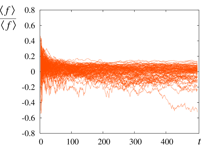
(b)  

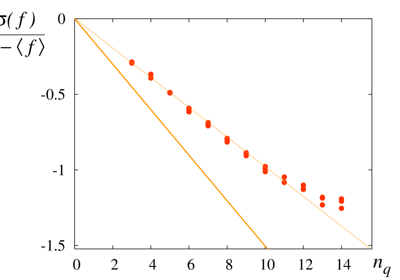
Figure 1: (Color online) 
(a) Ratio $\frac{f-\langle{f}\rangle}{1-\langle{f}\rangle}$, where $f$ is the unaveraged fidelity and $\langle{f}\rangle$ is its theoretical value given by formula 17, for $100$ numerical simulations on a sawtooth map with $n_{q}=12$ and $\epsilon=0.002$. As in the other numerical simulations in this article involving the sawtooth map, the number of cells is $L=2$, the classical parameter is $K=0.04$, the fidelity is observed in position representation and the initial state is $H\otimes\mathbb{I}\otimes H^{\otimes(n_{q}-2)}|\,0\,\rangle$; see appendix A for further details. The same behaviour (a spread depending only on the number of qubits for $N_{g}\gg 1$) was found for all the numerical simulations used in figure 1-b. The largest fluctuations tend to be located below the average.
(b) Values of $\frac{\sigma(f)}{1-\langle{f}\rangle}$, each point corresponding to $676$ numerical simulations at fixed error intensity $\epsilon$ and number of qubits $n_{q}$ ($\langle{f}\rangle$ is the numerical average of $f$). For each $n_{q}$ in $\{3,\dots,14\}$, the error intensities $\epsilon=0.002$, $0.005$ and $0.01$ were tried. Formula 20 predicts that these points depend only on $n_{q}$. The exact dependence $\sqrt{1/N}$, thick line, is however poorly followed. The thin line shows a fit with an exponential function $aN^{-b}$, giving $a\sim 1$ and $b\sim 1/3$.

The described fidelity decay model has been tested numerically on two algorithms simulating periodically driven quantum system: the sawtooth map Benenti et al. (2001) and the double-well map Chepelianskii and Shepelyansky (2002). These systems are usually studied in the quantum chaos field, because in spite of their relative simplicity they show a large variety of physical phenomena, from dynamical localisation to quantum ergodicity, first studied on the kicked rotator model maps_phenomena . If $\hat{\eta}$ and $\hat{\theta}$ are momentum and coordinate operators, then the evolution corresponding to one map step for a map with potential $V(\theta)$ is given by

$$\hat{U}_{F}=\exp\left(-i\frac{\hat{\eta}^{2}}{2\hbar}T\right)\exp\left(-i\frac{kV(\hat{\theta})}{\hbar}\right)$$

(see formula 24 and other physics and implementation details in appendix A). The behaviour of the classical counterparts of these chaotic maps is controlled by a single parameter $K=kT$, which in the following simulations is set to $0.04$. For this value, the double-well map presents a mixed phase space, with a large island of integrable motion in a chaotic sea; the sawtooth map is chaotic for every $K>0$, but the cantori regime extends up to $K\sim 1$, so that the presented numerical data best describe a perturbative regime. In both cases, it is not evident that the success of the uniform measure approximation depends on “chaos”.

The algorithms corresponding to the simulation of these maps contain the Fourier transform as a basic ingredient for changing the representation from coordinate to momentum and back. Since the simulated maps have periodic impulsive kicks, it is possible to write the overall evolution as a piecewise diagonal unitary transformation in the appropriate representation. The set of elementary gates which are used for the algorithms implementation contains single and double qubit phase shifts and Hadamard gates (see appendix C for more details). Since these algorithms are periodic, the results are usually expressed in terms of the number of gates $n_{g}$ per maps step. In the following the variable $t$ will be used when referring to the “map time” (the number of map steps). It is immediate to specialise the previous results for a map simply by replacing $N_{g}$ with $n_{g}t$. The effective decoherence parameter $\Gamma$ is defined by $f\sim 1-\Gamma t$.

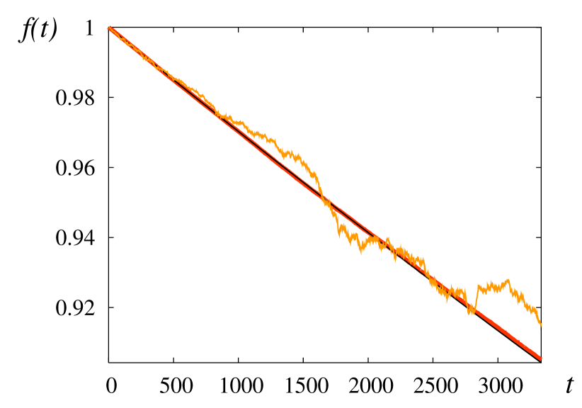
Figure 2: (Color online) Decay of the fidelity due to n.g. during the simulation of the sawtooth map, with $n_{q}=10$ and $\epsilon=0.003$. The simulation of one map step for such $n_{q}$ requires $n_{g}=200$ gates, with $n_{1}=45$ 1q gates and $n_{2}=155$ 2q gates. The value of $\Gamma$ from formula 17 is therefore $\simeq\epsilon^{2}n_{g}/59.6$, shown by the straight line. The red (dark) curve corresponds to an average over $500$ numerical simulations (it is hardly distinguishable from the straight line in this picture), while the orange (light) curve to a single try. See figure 1-a for the map parameters.

As a first check, the theoretical predictions were compared with the results of the simulation of a sawtooth map. This map is similar to the double-well map but it is free from the complications of using auxiliary qubits. Figure 1 is a check of formula 20; it shows that indeed the ratio $\sigma(f_{N_{g}})/(1-\langle{f_{N_{g}}}\rangle)$ depends only on $n_{q}$ and is exponentially small with it, but the theory predicts a decrease like $N^{-1/2}$ while $N^{-1/3}$ is observed. A possible explanation could be that the vectors $|\,\psi^{k}_{\perp}\,\rangle$ do not explore the complete $(N-1)$-dimensional space orthogonal to $|\,\psi^{k}\,\rangle$, but only $\sim N^{2/3}$ dimensions.

(a)  
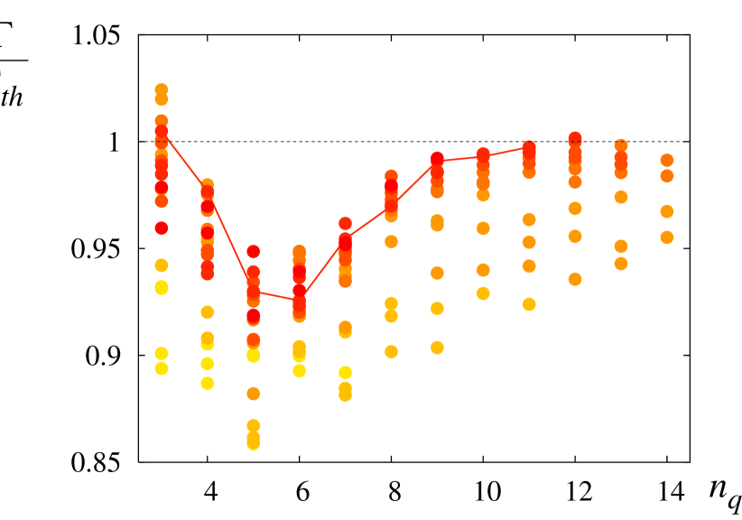
(b)  
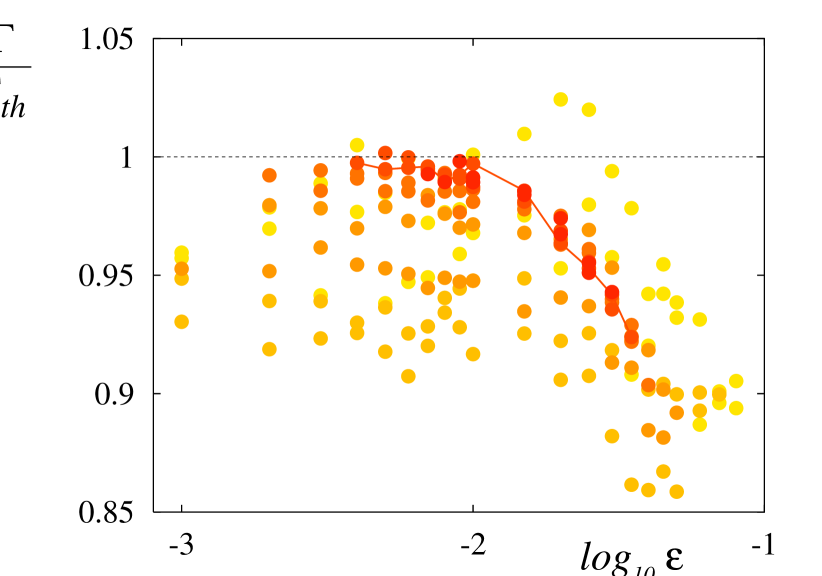
(c)  

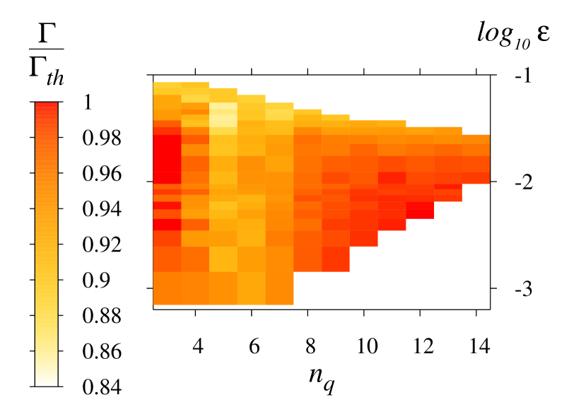
Figure 3: (Color online) 
(a) Ratio $\Gamma/\Gamma_{th}$ versus number of qubits $n_{q}$ for the sawtooth map. $\Gamma$ is the (numerical) fidelity decay constant and $\Gamma_{th}$ is its theoretical average, given by formula 17. Each point corresponds to an average at fixed $n_{q}$ and $\epsilon$ with $500$ numerical simulations. Yellow (light) points correspond to large errors ($\epsilon\sim 10^{-1}$) while red (dark) points to small errors ($\epsilon\sim 10^{-3}$). The solid line is an eye-guide for $\epsilon=0.004$. See figure 1-a for the map parameters.
(b) Same as picture 3-a, but the independent variable is the error intensity $\epsilon$, while the yellow to red (light to dark) transition corresponds to an increasing number of qubits. The solid line is an eye-guide for $n_{q}=11$. See figure 1-a for the map parameters.
(c) Same as picture 3-a/b, but the dependence on the error intensity $\epsilon$ and the number of qubits $n_{q}$ is shown at the same time. Each coloured box corresponds to an average at fixed $n_{q}$ and $\epsilon$ with $500$ numerical simulations. The yellow to red (light to dark) transition corresponds to an increasing value of the ratio, which remains however in general limited by $1$. Missing boxes are due either to combinations taking too long to simulate or to fidelities dropping too fast. See figure 1-a for the map parameters.

The previous ratio characterises the difficulty of fitting $\Gamma$ from a single numerical simulation, and can be used to estimate the number $n_{sim}$ of tries necessary to reduce the statistical uncertainty, for instance setting $\frac{1}{\sqrt{n_{sim}}}\frac{\sigma(f)}{1-\langle{f}\rangle}\sim 1\%$. This prescription implies a number of simulations $n_{sim}\sim 10^{4}2^{-n_{q}}$; however, it is better to use the numerical values from figure 1-b, because the theoretical formula gives an underestimate. In the remaining of the article $n_{sim}$ varies between $50$ to $500$.

An example of the degradation of the fidelity for the sawtooth map is given in figure 2, where it can be clearly seen that a single numerical simulation can give a fidelity which is not monotonic and correlated over many map steps. The prediction $\Gamma=An_{g}\sigma_{\ast}^{2}$, given by formula 17, is compared with numerical simulations, again for the sawtooth map, in figure 3. It turns out that the theoretical value is an upper bound for the the numerical fidelity decay constant, and that, not surprisingly, the agreement is better for a large number of qubits and small errors; for $n_{q}\gtrsim 10^{1}$ and $\epsilon<10^{-2}$, the discrepancy is within $5\%$.

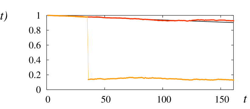
Figure 4: (Color online) Comparison of a typical and anomalous decay of the fidelity for the double-well map, with $n_{q}=5$ (plus one ancilla) and $\epsilon=0.01$. Both curves correspond to a single numerical simulation. The anomalous drop is due to a measurement of the ancilla giving the “wrong” result (note the change in the vertical scale). As in the other numerical simulations, unless otherwise stated, the number of cells is $L=2$, the classical parameter is $K=0.04$, the centre of the potential well is $a=1.6$, the fidelity is observed in position representation and the initial state is $H\otimes\mathbb{I}\otimes H^{\otimes(n_{q}-2)}|\,0\,\rangle$ (see appendix A).

The simulation of the fidelity decay on the double well map presents a new effect: beyond “standard” fidelity fluctuations, there are some rare “anomalous” fluctuations, like that in figure 4, with the fidelity dropping abruptly to almost zero. This is due to the fact that the algorithm implementation, for $n_{q}\geq 4$, uses an auxiliary qubit (an ancilla), which is reinitialised to $|\,0\,\rangle$ every time it is reused; the reinitialisation implies a measurement, which, when the evolution is affected by noise, can select the “wrong” result (i.e. $|\,1\,\rangle$), thus in practice completely destroying the computation. These catastrophic events become more and more frequent while $\epsilon$ increases.

However, when the measurement of the ancilla gives the “good” result, it turns out that the degradation of the fidelity is slowed down. This cancellation of the (unwanted) evolution is known as Zeno or watchdog effect zeno_origin ; recently it has been shown that this inhibition of decoherence can arise in more general contexts, where the essential ingredient is a strong coupling to the environment and not its trivial dynamics zeno_general . In the simulation of the double-well map it is indeed the ancilla which plays the role of the environment.

The repeated observation of the ancilla can be thought of as an error correction strategy in the Zeno regime Erez et al. (2003), because the q.c. memory state is partially rectified even when the measurement gives the expected result. The Zeno effect is known to be linked to error correction from the very early days of quantum computation zeno_and_qc ; it has been suggested as a stabilisation strategy by Shor Shor (1997) in his famous paper on prime factoring, in a context identical to the current one (i.e. syndrome measurement without a recovery circuit).

Of course, a direct observation of a fidelity jump, like that in figure 4, is not possible on a real q.c. It is true that the result of each ancilla measurement is accessible, so one could decide to purge a set of real experiments of those instances which showed a “faulty” reinitialisation; another option could be not to reinitialise the ancilla at all. In any case, the only meaningful quantity is the average fidelity.

(a)  
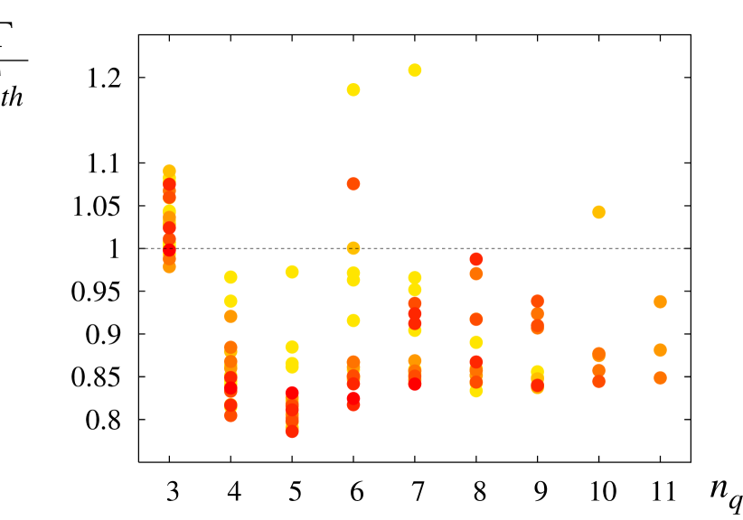
(b)  
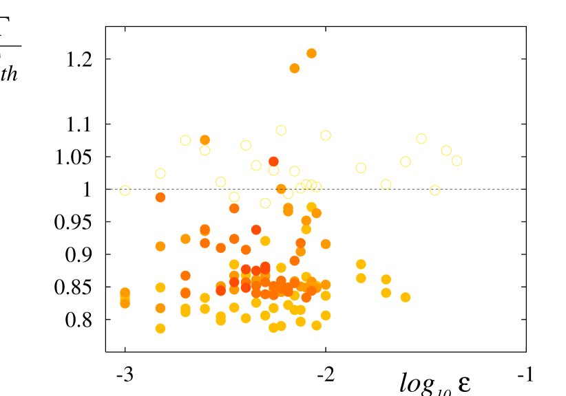
(c)  

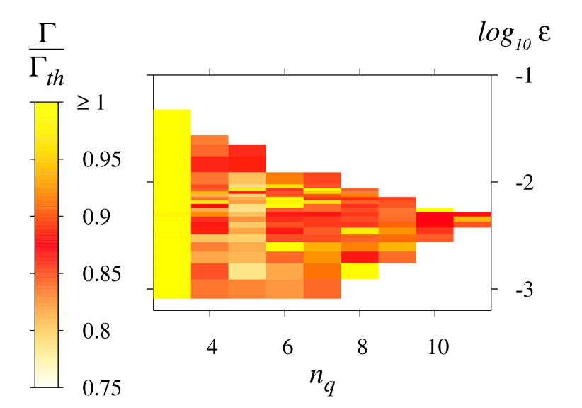
Figure 5: (Color online) 
(a) Ratio $\Gamma/\Gamma_{th}$ versus number of qubits $n_{q}$ for the double-well map. $\Gamma$ is the (numerical) fidelity decay constant and $\Gamma_{th}$ is its theoretical average, given by formula 17. Each point corresponds to an average at fixed $n_{q}$ and $\epsilon$ with $200$ numerical simulations; at least $20$ map iterations can be simulated before $f$ drops below $0.9$. Yellow (light) points correspond to large errors ($\epsilon\sim 10^{-1}$) while red (dark) points to small errors ($\epsilon\sim 10^{-3}$). For $n_{q}=3$ the algorithm does not use ancillae.
(b) Same as picture 5-a, but the independent variable is the error intensity $\epsilon$, while the yellow to red (light to dark) transition corresponds to an increasing number of qubits. Most of the points for $n_{q}\geq 4$ (filled circles) lie in the $80\%-90\%$ region, with a preference for $\sim 85\%$. Empty circles correspond to the case $n_{q}=3$ (no ancilla).
(c) Same as picture 5-a/b, but the dependence on the error intensity $\epsilon$ and the number of qubits $n_{q}$ is shown at the same time. Each coloured box corresponds to an average at fixed $n_{q}$ and $\epsilon$ with $200$ numerical simulations. The orange and red (dark) boxes correspond to a $\Gamma$ which is $\sim 15\%$ smaller than its theoretical value due to the reinitialisations of the ancilla (Zeno effect). For $n_{q}=3$ the algorithm implementation does not use ancillae. Missing boxes are due either to combinations taking too long to simulate or to fidelities dropping too fast.

The numerical simulations presented in this article are not purged of the unwanted reinitialisations. This slow-down is illustrated in figure 5, where the numerically found value of $\Gamma$ is approximately $10\%$ to $20\%$ smaller than the prediction of formula 17, with a preference for $\sim 15\%$. Note that for $n_{q}=3$ the algorithm implementation does not use ancillae, and the result is in agreement with what was found for the sawtooth map (figure 3). “Wrong measurement” events, like that shown in figure 4, become more and more frequent in the averaging ensemble for large error intensities.

V Conclusions

In this article the degradation of the performance of a q.c. affected by n.g. is investigated, both analytically and numerically, by studying the fidelity of the noisy states with respect to the ideal state (definition 1): the average value of the fidelity after a fixed number of elementary gates characterises the “precision” of the q.c. and can be efficiently extracted from a set of experiments via forward-backward evolution. The numerical tests are performed using two algorithms that simulate the sawtooth and the double-well maps. In the following $n_{q}$ is the number of qubits in the q.c. and $N=2^{n_{q}}$ is the number of states.

The degradation of the fidelity is shown to be determined basically by $\sigma_{\ast}^{2}$, the mean variance of the phases of the eigenvalues of the error operators (definition 11); stated in this way, this result is valid for every choice of elementary gates. In a realistic case, where the q.c. is endowed with a particular set of elementary operations, each characterised by a specific error operator distribution, this quantity is algorithm-dependent only through the relative frequencies of the elementary gates; so, $\sigma_{\ast}^{2}$ reflects the effective decoherence inherent to the q.c, and a careful analysis of the results of different algorithms would allow in principle to determine the proper $\sigma_{\ast}^{2}$ for each gate type.

The noise-averaged fidelity after $N_{g}$ elementary gates is found to be $\langle{f_{N_{g}}}\rangle=1-\frac{N}{1+N}N_{g}\sigma^{2}_{\ast}+O(\sigma^{3}_{\ast})$. The fluctuations of the value of the fidelity after a fixed number of gates are such that $\sigma(f)/(1-\langle{f}\rangle)$ depends only on $n_{q}$ and is exponentially small with it. It is also found that the reinitialisation of the auxiliary qubit during the computation for the double-well map reduces the fidelity decay rate of $\sim 15\%$ (this is known in literature as an error correction in the Zeno regime).

Note that a particular case of distribution of the error operators is the one which does not depend on the gate type (this case bears the additional bonus that there is no dependence at all on the algorithm). In this scenario, an ensemble of unitary errors is equivalent to the more commonly studied case of a non-unitary error channel, like for instance the depolarisation channel.

The rather good agreement between the quantitative predictions of the theory and the numerical results for the double-well and sawtooth maps suggests a general validity for the assumption on the distribution of the states visited by an algorithm. It is clear however that there exist trivial algorithms which do not follow the predicted behaviour for some choice of their initial state. The question is then to characterise the class of algorithms which satisfy well enough the predictions, and, in particular, to understand whether this is linked or not to the fact that the algorithms used as examples exploit the q.c. in order to simulate another quantum system, showing ergodic properties. Due to the robustness of the prediction for $\sigma_{\ast}^{2}$ for state distributions close to the uniform distribution, the conjecture is that the class is not limited to this type of algorithms.

It would be interesting to extend the ideas presented in this article in order to include measurements of auxiliary qubits; as shown by numerical simulations, measurements of qubits supposed to be, in absence of errors, in a known state can slow down the fidelity decrease. In perspective, this could allow to deal with error correction codes, a subject which has not been treated here.

The numerical simulations in this article were performed using a freely available implementation of the quantum programming language described in Bettelli et al. (2003). The author acknowledges useful discussions with A. Pomeransky, M. Terraneo, B. Georgeot and J. Emerson.

This work was supported in part by the European Union RTN contract HPRN-CT-2000-0156 (QTRANS) and IST-FET project EDIQIP, and by the French government ACI (Action Concertée Incitative) Nanosciences-Nanotechnologies LOGIQUANT.

Appendix A Hamiltonian maps as quantum algorithms

The goal of this appendix is to show the general approach to build a quantum algorithm for a quantum Hamiltonian map derived from a classical unidimensional kicked map. A classical kicked map is the stroboscopic observation of the phase space of a system which is affected by an impulsive conservative force given by a periodic potential at regular intervals in time and which evolves freely in the meanwhile. If the observation occurs just before the kick, the map connecting the points in the dimensionless $(\theta,\eta)$ phase space can be written, without loss of generality, as

$$\left\{\begin{array}[]{lll}\bar{\eta}&=&\eta-k\frac{dV}{d\theta}\\ \bar{\theta}&=&\theta+T\bar{\eta}\pmod{2\pi}\end{array}\right.$$ (22)

In this expression, $T$ represents the (dimensionless) time interval between two kicks, $2\pi$ is the period of the potential $V(\theta)$ and $k$ is a parameter which governs the intensity of the potential. It is easy to show that, if the rescaled variable $\eta^{\prime}=T\eta$ is used instead of $\eta$, the map depends on one parameter only, that is $K=kT$. In the map 22 the $\theta$ range is finite, while the momentum $\eta$ can vary arbitrarily. However, the transformation

$$(\theta,\eta)\rightarrow(\theta,\eta+2\pi L/T),\quad\quad L\in\mathbb{Z},$$ (23)

is a symmetry for the system; this invariance identifies a natural cell, with an extension of $2\pi$ in both directions of the phase space, and $L$ can therefore be associated to the number of cells. The time-dependent classical Hamiltonian driving the evolution described by the map 22 is

$$H(\theta,\eta,t)=\frac{\eta^{2}}{2}+kV(\theta)\sum_{j=-\infty}^{+\infty}\delta(t-jT).$$

The map quantisation can be accomplished by replacing the dynamical variables $\theta$ and $\eta$ with the corresponding operators $\hat{\theta}$ and $\hat{\eta}$. In the $\theta$ representation, the momentum operator becomes, as usual, $\hat{\eta}=-i\frac{\partial}{\partial\theta}$. The quantum equivalent of the map 22 is the evolution operator calculated for a time interval $T$ (which includes always one kick), known as the Floquet operator ($U_{F}$). Given that the action of the potential is impulsive, the integration of the quantum Hamiltonian is very easy:

$$\hat{U}_{F}=\exp\left(-i\frac{\hat{\eta}^{2}}{2\hbar}T\right)\exp\left(-i\frac{kV(\hat{\theta})}{\hbar}\right).$$ (24)

Therefore, in the quantum case the dynamics is determined not only by the product $K=kT$, but also by the “magnitude” of $\hbar$ (for instance, by the ratio $k/\hbar$).

The simulation of the quantum map on a finite q.c. implies some type of discretisation, which introduces an additional parameter, namely the number of available levels, $N=2^{n_{q}}$. The easiest choice is to associate the computational basis states $|\,i\,\rangle$ to some eigenvalue $\theta_{i}$. In this way the “position” operator $\theta$ becomes diagonal in the computational basis. In the algorithm described in this article the following choice holds:

$$|\,i\,\rangle\quad\longrightarrow\quad\theta_{i}=\frac{2\pi}{N}(i+\delta_{\theta}).$$ (25)

In this way the position eigenvalues are equidistant; $\delta_{\theta}$ is an offset which fixes the exact $2\pi$ interval where the eigenvalues are located. The choice $\delta_{\theta}=(1-N)/2$ corresponds to $-\pi<\theta_{i}<\pi$, with perfect symmetry around $\theta=0$. The periodicity condition $\theta\equiv\theta+2\pi$ implies that the eigenvalues of the momentum must be quantised in units of $\hbar$. The finiteness of the q.c. memory allows only for a finite number $N$ of eigenvalues of the momentum to be simulated. It is therefore natural to resort to a cyclic condition, that is assuming that the range of the eigenvalues corresponds to an integer number of cells (see the transformation 23):

$$\Delta\eta=N\hbar=2\pi L/T\quad\quad\Rightarrow\quad\quad T\hbar=\frac{2\pi L}{N}.$$ (26)

The last step in the construction of the algorithm is the fact that the quantum Fourier transform $\mathcal{F}$ “exchanges” the momentum representation with the position representation. This means that if, at some time during the simulation, the q.c. memory’s state is $|\,\psi\,\rangle=\sum_{j}a_{j}|\,j\,\rangle$ and it is associated to the simulated system’s state $\sum_{j}a_{j}|\,\theta_{j}\,\rangle$, where the $|\,\theta_{j}\,\rangle$’s are the eigenstates of $\hat{\theta}$ with eigenvalue $\theta_{j}$, then $\mathcal{F}^{\dagger}|\,\psi\,\rangle=\sum_{j}b_{j}|\,j\,\rangle$ must be associated to the simulated system’s state $\sum_{j}b_{j}|\,\eta_{j}\,\rangle$, where the $|\,\eta_{j}\,\rangle$’s are the eigenstates of $\hat{\eta}$ with eigenvalue $\eta_{j}=j\hbar$. In other words, the Floquet operator $\hat{U}_{F}$ (see 24) can be simulated by a quantum circuit $Q$ whose action is:

$$Q = \mathcal{F}\circ Q_{\eta}\circ\mathcal{F}^{\dagger}\circ Q_{\theta}$$ (27)

$$Q_{\eta}|\,j\,\rangle = \exp\left(-i\frac{\eta_{j}^{2}}{2\hbar}T\right)|\,j\,\rangle$$ (28)

$$Q_{\theta}|\,j\,\rangle = \exp\left(-i\frac{kV(\theta_{j})}{\hbar}\right)|\,j\,\rangle$$ (29)

$$\mathcal{F}|\,j\,\rangle = \frac{1}{\sqrt{N}}\sum_{m}e^{2\pi i\frac{jm}{N}}|\,m\,\rangle$$ (30)

It is now useful to define an operator $\mathcal{U}\left(\beta,p\right)$ as

$$\mathcal{U}\left(\beta,p\right)|\,j\,\rangle=\exp\left(2\pi i\beta j^{p}\right)|\,j\,\rangle.$$ (31)

The circuit $Q_{\eta}$ acting in the momentum representation (see equation 28) can then be simplified by using the definition 31, and replacing the eigenvalue $\eta_{j}$ with $j\hbar$ and the product $T\hbar$ with the help of expression 26:

$$Q_{\eta}|\,j\,\rangle=\exp\left(-2\pi i\frac{L}{2N}j^{2}\right)|\,j\,\rangle=\mathcal{U}\left(\frac{-L}{2N},2\right)|\,j\,\rangle.$$ (32)

In this expression the parameters $T$ and $\hbar$ have been replaced by the number of levels $N$ and the number of cells $L$: the free evolution is thus completely geometrical. The (dimensionless) quantum action $\hbar$ is proportional to $L/N$, therefore the semi-classical limit can be attained by taking $L/N\rightarrow 0$.

The circuit $Q_{\theta}$ (see equation 29) is easy to manage when the potential $V(\theta)$ of the map 22 is a polynomial in $\theta$ (let $p$ be its degree). One can in fact introduce the polynomial $\mathcal{P}(x+\delta_{\theta})=\sum_{m=0}^{p}f_{m}x^{m}$ and set

$$V(\theta_{j})=V\left(\frac{2\pi}{N}(j+\delta_{\theta})\right)=\left(\frac{2\pi}{N}\right)^{p}\mathcal{P}(j+\delta_{\theta}),$$

where $\theta_{j}$ has been replaced with expression 25. The circuit $Q_{\theta}$ (see equation 29) can then be broken down into circuits of type $\mathcal{U}\left(\beta,m\right)$ (see the definitions 31 and 26 and remember that $K=kT$):

$$Q_{\theta}|\,j\,\rangle = \exp\left(-i\frac{KV(\theta_{j})}{2\pi L/N}\right)|\,j\,\rangle$$ (33)

$$= \prod_{m=1}^{p}\mathcal{U}\left(\frac{-Kf_{m}(2\pi)^{p-2}}{LN^{p-1}},m\right)|\,j\,\rangle.\qquad$$

Note that the term $m=0$, which gives only a global phase, can be neglected. For the double-well Chepelianskii and Shepelyansky (2002) map ($p=4$) the polynomial is:

$$\mathcal{P}(y)=\left(y^{2}-a^{2}\right)^{2},$$

where $a$ is an additional parameter which locates the centres of the two wells. The coefficients $f_{m}$ are therefore

$$f_{4}=1,\quad f_{3}=4\delta_{\theta},\quad f_{2}=6\delta_{\theta}^{2}-2a^{2},\quad f_{1}=4\delta_{\theta}(\delta_{\theta}^{2}-a^{2}).$$

For the sawtooth Benenti et al. (2001) map ($p=2$) the polynomial and the coefficients are respectively

$$\mathcal{P}(y)=-\frac{1}{2}y^{2},\quad f_{2}=-\frac{1}{2},\quad f_{1}=-\delta_{\theta}.$$

Summarising, it has been shown that the circuit $Q$ (equation 27) can be written as a composition of circuits for the Fourier transform $F$ (equation 30) and for the operators $\mathcal{U}\left(\beta,m\right)$ (equation 31). The parameters which govern the simulation are the classical parameter $K$ (integrability $\rightarrow$ chaos), the number of simulated cells $L$ and the number of available levels $N$ ($L/N\rightarrow 0$ being the semi-classical limit) in addition, of course, to the functional form of the potential $V(\theta)$.

The state of the q.c. memory after each application of the circuit $Q$ corresponds to the coordinate representation for the simulated system, but trivial changes allow the simulation in the momentum representation. It is well known that the circuit for $\mathcal{F}$ can be implemented efficiently Coppersmith (1994). Appendix B shows that also $\mathcal{U}\left(\beta,m\right)$ can be implemented efficiently; the conclusion is therefore that the circuit for the simulation of a quantum kicked Hamiltonian with a polynomial potential can be implemented efficiently on a q.c.

There exist, of course, interesting potentials which are not polynomial; for instance, the kicked rotator map has $V(\theta)=\cos\theta$. For this case, two approaches are known. In Georgeot and Shepelyansky (2001a) an auxiliary register and a number of additional ancillae is used for calculating $|\,\theta\,\rangle|\,0\,\rangle\rightarrow|\,\theta\,\rangle|\,\cos\theta\,\rangle$ with a finite number of digits in the mantissa; the auxiliary register is subsequently used to implement $Q_{\theta}$. If the size of the mantissa for the calculation of the cosine is $O(n_{q})$, the circuit depth is $O(n_{q}^{3})$ and the number of ancillae is $O(n_{q})$. In Pomeransky and Shepelyansky (2003) another approximated method, with circuit depth $O(kn_{q})$, is introduced. This method is very interesting because no auxiliary qubit is required; however, the precision with which $Q_{\theta}$ is implemented is $O(k)$, so the approach is optimal only for small $k$ values.

Appendix B A quantum circuit for exponentiation

The goal of this appendix is to show a procedure for building an efficient quantum circuit implementing the unitary transformation

$$\mathcal{U}\left(\beta,p\right)|\,x\,\rangle=e^{2\pi i\beta x^{p}}|\,x\,\rangle.$$ (34)

In expression 34, the exponent $p$ is a positive integer while $\beta$ is a real coefficient. $|\,x\,\rangle$ is the $x$-th element of the computational basis, therefore $\mathcal{U}\left(\beta,p\right)$ is diagonal in this basis. The circuit is implicitly parametrised by the number $n_{q}$ of qubits in the register which $\mathcal{U}\left(\beta,p\right)$ operates on. The first step is to write the integer $x$ labelling $|\,x\,\rangle$ as a binary string, $x=\sum_{j=0}^{n_{q}-1}a_{j}2^{j}$. By replacing this expression into the phase of definition 34, it is possible to rewrite it as the product:

$$e^{2\pi i\beta x^{p}}=\prod_{j_{1}\dots j_{p}}e^{2\pi i\beta a_{j_{1}}\dots a_{j_{p}}2^{j_{1}+\dots+j_{p}}}.$$

Since the coefficients $a_{j}$ are binary digits, the product $a_{j_{1}}\dots a_{j_{p}}$ is zero (i.e. the phase is trivial) unless all the $a_{j}$’s are equal to $1$. Therefore each factor in the previous expression corresponds to a multi-controlled phase gate in the circuit for $\mathcal{U}\left(\beta,p\right)$ of definition 34. This gate acts on the qubits selected by the set $W(j_{1}\dots j_{p})$, which contains the values of the indexes $j_{1}$, …$j_{p}$ with neither repetitions nor order. Introducing the notation $\mathcal{C}_{W}(\varphi)$ for a multi-controlled phase gate applying the phase $\exp(2\pi i\varphi)$ to the qubits in the set $W$, one obtains

$$\mathcal{U}\left(\beta,p\right)=\prod_{j_{1}\dots j_{p}}\mathcal{C}_{W(j_{1}\dots j_{p})}(\beta 2^{j_{1}+\dots+j_{p}}).$$ (35)

Up to now, this method follows exactly the procedure described in Chepelianskii and Shepelyansky (2002). The set $W$ does not contain duplicated elements, so that its cardinality is smaller or equal to $p$ (but it is always positive). Since neither the sum $j_{1}+\dots+j_{p}$ nor the set $W(j_{1}\dots j_{p})$ depend on the order of the indexes, all the gates concerning the same indexes and differing only in their order can be collected into a single gate. Let

$$P=\left\{J\subset\{0,...,n_{q}-1\}|J\neq\emptyset\wedge\left|J\right|\leq p\right\},$$ (36)

where $0\dots n_{q}-1$ are the possible values for the qubit indexes. Then expression 35 can be rewritten as

$$\mathcal{U}\left(\beta,p\right) = \prod_{J\in P}\prod_{\begin{subarray}{c}j_{1}\dots j_{p}\\ W(j_{1}\dots j_{p})=J\end{subarray}}\mathcal{C}_{W(j_{1}\dots j_{p})}(\beta 2^{j_{1}+\dots+j_{p}})$$ (37)

$$= \prod_{J\in P}\mathcal{C}_{J}\Big{(}\beta\sum_{\begin{subarray}{c}j_{1}\dots j_{p}\\ W(j_{1}\dots j_{p})=J\end{subarray}}2^{j_{1}+\dots+j_{p}}\Big{)},$$

where in the last line the gates with the same $J$ have been compressed into a single gate. Note that two gates act on the same qubits if and only if their $W$ sets are equal. To proceed, one needs to define the set $G_{k}(n)$ of the partitions of $n$ objects in exactly $k$ non-empty subsets. A partition $g\in G_{k}(n)$ is then a sequence of $k$ positive integers $\{g_{1}\dots g_{k}\}$ such that their sum is equal to $n$. Given a set $J$ and a partition $g\in G_{\left|J\right|}(p)$, the pair $\langle J,g\rangle$ corresponds to a subdivision of the set of $p$-tuples whose $W$ set is $J$. It is then possible to apply the replacement

$$\sum_{\begin{subarray}{c}j_{1}\dots j_{p}\\ W(j_{1}\dots j_{p})=J\end{subarray}}\quad\longrightarrow\quad\quad\sum_{g\in G_{\left|J\right|}(p)}\sum_{\begin{subarray}{c}j_{1}\dots j_{p}\\ W(j_{1}\dots j_{p})=J\\ j_{1}+\dots+j_{p}=\sum g_{i}J_{i}\end{subarray}}$$ (38)

For each pair $\langle J,g\rangle$, the sum $j_{1}+\dots+j_{p}$ is fixed, therefore the last summation on the right of expression 38 can be replaced by its multinomial weight $\frac{p!}{g_{1}!\cdots g_{\left|J\right|}!}$. Putting all together, one finally obtains that the operator $\mathcal{U}\left(\beta,p\right)$ can be replaced by a product of multi-controlled gates $\mathcal{C}_{J}(\varphi)$, with a bijective correspondence between the gates and the sets $J\in P$, where

$$\varphi=\beta\sum_{g\in G_{\left|J\right|}(p)}\frac{p!}{g_{1}!\cdots g_{\left|J\right|}!}\,2^{\sum g_{i}J_{i}}.$$ (39)

This gate collection method presents the obvious advantage that the circuit depth decreases. In fact, if one gate is built for each possible index combination $j_{1}\dots j_{p}$, the total number of gates is trivially $(n_{q})^{p}$. If, on the other hand, the previously described compression is applied, one obtains as many gates as the cardinality of the set of partitions $P$ (definition 36), i.e.

$$\left|P\right|=\sum_{k=1}^{\min(n_{q},p)}\binom{n_{q}}{k}.$$ (40)

For $n_{q}\leq p$ this sums to $2^{n_{q}}-1$. However, it is more interesting to consider the limit $n_{q}\gg p$; approximating the sum with the help of Stirling’s formula one obtains

$$\left|P\right|\sim\frac{(n_{q})^{p}}{p!}.$$

It is easy to check that this approximation is already good for $n_{q}=5$ and $p=4$, where the savings $1/p!$ correspond to $\sim 95\%$ of the gates. It should be kept in mind that the calculation of $\varphi$ in expression 39 can be numerically critical, because for large $n_{q}$ the integer multiplying $\beta$ grows exponentially as $2^{pn_{q}}$. Since this phase term is to be taken modulo 1, the least significant bits of the representation of $\beta$ are to be handled carefully.

In practice however, when $\mathcal{U}\left(\beta,p\right)$ is used as a block of a larger circuit, like 32 or 33, $\beta$ is also exponentially small. For $p\geq 2$ the worst case comes from circuit 32, where $\beta=O(2^{-n_{q}})$, so that the phase $\varphi$ is $O(2^{n_{q}(p-1)})$. If $\beta$ is stored as a floating point number, one loses $p-1$ bit of the mantissa of $\varphi$ for every qubit added. For a double precision floating point this problems arises around $n_{\mathrm{crit}}=18$ for the double-well map and around $n_{\mathrm{crit}}=53$ for the sawtooth map. This is beyond or at the limit of the possibilities of current q.c. simulators. In any case, the study of the real degradation of a computation due to this loss of precision in the most critical gates for $n_{q}>n_{\mathrm{crit}}$ is not trivial and has not been performed yet.

Appendix C Error models and bounds to the fidelity degradation

In all the numerical simulations of this article, it is supposed that the q.c. is endowed with the following set of hardware operations:

$$H=\frac{1}{\sqrt{2}}\left(\begin{smallmatrix}1&\phantom{-}1\\ 1&-1\end{smallmatrix}\right)\quad R_{\phi}=\left(\begin{smallmatrix}1&\\ &\!e^{i\phi}\!\!\end{smallmatrix}\right)\quad CR_{\phi}=\left(\begin{smallmatrix}1&&&\\ &1&&\\ &&1&\\ &&&\!e^{i\phi}\!\!\end{smallmatrix}\right),$$

where $\phi\in\mathbb{R}$ is a phase (indeed, it can be only a multiple of some “atomic” phase, like $2\pi/2^{32}$, which mimics the limited precision of the classical control system). $H$ is the Hadamard transformation, while $R_{\phi}$ and $CR_{\phi}$ are phase shifts and controlled phase shifts respectively. In general, the controlled operation $CA$ corresponds to the matrix $\left(\begin{smallmatrix}\mathbb{I}&\\ &A\end{smallmatrix}\right)$. It is sometimes useful to express the elementary gates as rotations $R_{\hat{\eta}}(\alpha)$ of an angle $\alpha$ around an axis $\hat{\eta}$:

$$R_{\hat{\eta}}(\alpha)=e^{-i\frac{\alpha}{2}\hat{\eta}\cdot\vec{\sigma}}=\cos\left(\frac{\alpha}{2}\right)-i\sin\left(\frac{\alpha}{2}\right)\hat{\eta}\cdot\vec{\sigma}.$$

With this notation, setting $\widehat{xz}=(\hat{x}+\hat{z})/\sqrt{2}$, one finds $H\!=e^{i\frac{\pi}{2}}R_{\widehat{xz}}(\pi)\equiv R_{\widehat{xz}}(\pi)$ and $R_{\phi}=e^{i\frac{\phi}{2}}R_{\hat{z}}(\phi)\equiv R_{\hat{z}}(\phi)$, where ’$\equiv$’ means equivalence modulo a global phase (which can be neglected). Note, however, that $CR_{\phi}=e^{i\frac{\phi}{4}}[R_{\hat{z}}(\frac{\phi}{2})\otimes\mathbb{I}]\circ CR_{\hat{z}}(\phi)\not\equiv CR_{\hat{z}}(\phi)$, so that $CR_{\phi}$ and $CR_{\hat{z}}(\phi)$ are inequivalent even modulo a global phase.

In the n.g. error model (see for instance Song and Shepelyansky (2001)), each gate is replaced by a still unitary transformation, close in norm to the original gate, parametrised by a single error variate $\xi$ with flat probability in $[-\epsilon/2,\epsilon/2]$. The quantity $\epsilon$ is called the “error intensity”, and it summarises the amount of noise which affects the q.c. It is useful to express a perturbed elementary gate as a composition of the unperturbed gate followed by an error operator close to the identity. The imperfections for $z$-rotations and controlled $z$-rotations are implemented by shifting their phase angle by an amount $\xi$; it is easy to show that

$$\textrm{noisy\leavevmode\nobreak\ }R_{\phi} \longrightarrow R_{\xi}R_{\phi}\equiv R_{\hat{z}}(\xi)R_{\phi}\qquad\mathrm{and}$$

$$\textrm{noisy\leavevmode\nobreak\ }CR_{\phi} \longrightarrow CR_{\xi}CR_{\phi}\equiv\left[R_{\hat{z}}(\frac{\xi}{2})\otimes\mathbb{I}\right]CR_{\hat{z}}(\xi)\,CR_{\phi}.$$

Each Hadamard gate is transformed into a rotation of an angle $\pi$ around an axis $\hat{\eta}^{\prime}$ randomly tilted around the unperturbed direction $\hat{\eta}=\widehat{xz}$ of an angle $\xi/2$. The perturbed gates can be generated by taking a random direction $\hat{\mu}$ in the plane orthogonal to $\widehat{xz}$ and setting $\hat{\eta}^{\prime}=\hat{\eta}\cos\frac{\xi}{2}+\hat{\mu}\times\hat{\eta}\sin\frac{\xi}{2}$. Note that the signs of $\mu$ and $\xi$ are not independent. A little algebra shows that

$$\textrm{noisy\leavevmode\nobreak\ }H\longrightarrow R_{\hat{\mu}}(\xi)H.$$

Thus, the error operators $\mathcal{E}_{k}$ in the n.g. error model are $R_{\hat{z}}(\xi)$, $R_{\hat{\mu}}(\xi)$ and $CR_{\xi}$, the phases of the eigenvalues for 1q errors are $\{\pm\frac{\xi}{2}\}$, and those for 2q errors are $\{0_{3},\xi\}$. All these eigenvalues are of course specified modulo a global phase shift. It is easy to see that this model is unbiased. Another approach to n.g. Georgeot and Shepelyansky (2001b) consists in diagonalising the gates and perturbing the eigenvalues of an amount $\xi$; given that the average properties of the induced effective decoherence are determined only by the error operators’ spectrum, it is not surprising that this alternative approach yields in general very similar results. The calculation of the radius $r_{k}$ of the neighbourhood of the eigenvalue phases (see equation 9) is very simple; $r_{k}$ is always $|\xi|/2$, so that (see equation 6)

$$\varsigma_{\ast}\simeq\left\langle r_{k}\right\rangle=\frac{1}{\epsilon}\int_{\frac{\epsilon}{2}}^{\frac{\epsilon}{2}}\frac{|\xi|}{2}\,d\xi=\frac{\epsilon}{8}.$$ (41)

The incoherent replacement $(\sum_{k}\varsigma_{\ast k})^{2}\rightarrow(\sum_{k}\varsigma_{\ast k}^{2})$ in formula 7 gives the result necessary for formula 10:

$$1-f\leq N_{g}\left\langle\frac{\xi^{2}}{4}\right\rangle=\frac{N_{g}}{\epsilon}\int_{\frac{\epsilon}{2}}^{\frac{\epsilon}{2}}\frac{\xi^{2}}{4}\,d\xi=\frac{\epsilon^{2}N_{g}}{48}$$ (42)

Appendix D Uniform averages and concentration of measure

This appendix details the evaluation of an integral like

$$\mathcal{I}(\widehat{R}^{\,(1)},\dots,\widehat{R}^{\,(r)})=\int d\mu(\psi)\,\prod_{k=1}^{r}\langle\,\psi\,|\widehat{R}^{\,(k)}|\,\psi\,\rangle,$$ (43)

where the $\widehat{R}^{\,(k)}$ are operators over an $N$-dimensional Hilbert space, and $d\mu(\psi)$ is the uniform measure over its unity vectors (that is, the unique invariant measure under the action of all unitary matrices). If the integrand is expanded over some basis, then

$$\mathcal{I}(\widehat{R}^{\,(1)},\dots,\widehat{R}^{\,(r)})=\prod_{k}R^{\,(k)}_{i_{k}j_{k}}\cdot\underbrace{\int d\mu(\psi)\prod_{k}\psi^{*}_{i_{k}}\psi_{j_{k}}}_{T_{i_{1}j_{1}\dots i_{r}j_{r}}}\quad,$$

where the linearity of the expectation value and the fact that the average is over the $|\,\psi\,\rangle$’s and not over the $\widehat{R}^{\,(k)}$’s were used (summation over repeated indexes is understood). The measure $d\mu(\psi)$ over the Hilbert space can be turned into a measure $d\mu(U)$ over the set of unitary transformations of this space. Since $d\mu(\psi)$ is by definition invariant when $U|\,\psi\,\rangle$ is substituted for $|\,\psi\,\rangle$ in formula 43, with $U$ a generic unitary matrix, $d\mu(U)$ remain completely determined (Haar or uniform measure, corresponding to the unitary circular ensemble Mehta (1991)).

This invariance allows for the calculation of the averages 43 without a direct integration unitary_integrals . It can be shown Brouwer (1997) that the tensor $T_{i_{1}j_{1}\dots i_{r}j_{r}}$ must be proportional to a sum of products of Kronecker’s deltas symmetric with respect to the indexes of the same type (i.e. the $i$’s or the $j$’s); the normalisation coefficient can then be fixed by comparison with the case $\widehat{R}^{\,(k)}=\mathbb{I}\,\,\forall k$. For $r=1$

$$T_{ij}\propto\delta_{ij},\qquad\mathrm{therefore}\qquad\mathcal{I}(\widehat{R})=\frac{\mathrm{tr}(\widehat{R})}{N}.$$ (44)

For the case $r=2$ one similarly obtains

$$T_{ijkl}\propto(\delta_{ij}\delta_{kl}+\delta_{il}\delta_{jk}).$$

Thus, the integral 43 can be written using only traces:

$$R^{\,(1)}_{ij}R^{\,(2)}_{kl}T_{ijkl}=\frac{\mathrm{tr}(\widehat{R}^{\,(1)})\mathrm{tr}(\widehat{R}^{\,(2)})+\mathrm{tr}(\widehat{R}^{\,(1)}\widehat{R}^{\,(2)})}{N^{2}+N}.$$ (45)

If the operators are simultaneously diagonalisable, it is easy to see that the integral depends only on their spectrum. If $\widehat{R}$ is a generic unitary operator, setting $\mathcal{I}(\widehat{R},\widehat{R}^{\dagger})=\mathcal{I}_{2}(\widehat{R})$ and $A=\frac{N}{1+N}$ one obtains that

$$\mathcal{I}_{2}(\widehat{R})=1-A\Big{[}1-\frac{|\mathrm{tr}(\widehat{R})|^{2}}{N^{2}}\Big{]}.$$ (46)

When $\widehat{R}$ has only two eigenvalues, $e^{i\lambda_{1}}$ and $e^{i\lambda_{2}}$, with the same multiplicity $N/2$ (i.e., when it is a generic 1q operator), the previous formula reduces to

$$\mathcal{I}_{2}\left(\begin{smallmatrix}e^{i\lambda_{1}}&0\\ 0&e^{i\lambda_{2}}\end{smallmatrix}\right)=1-A\sin^{2}\left({\textstyle\frac{\lambda_{1}-\lambda_{2}}{2}}\right).$$ (47)

It is interesting to calculate the same integral in a different way. By introducing the probability $0\leq p\leq 1$ of being in the first eigenspace, the state can be written as

$$|\,\psi\,\rangle=\sqrt{p}\,|\,\psi_{1}\,\rangle+\sqrt{1-p}\,|\,\psi_{2}\,\rangle,$$

where the normalised state $|\,\psi_{j}\,\rangle$ is an eigenstate with eigenvalue $e^{i\lambda_{j}}$, and all the unnecessary phases have been reabsorbed. The integral in formula 47 becomes then

$$\mathcal{I}_{2}\left(\begin{smallmatrix}e^{i\lambda_{1}}&0\\ 0&e^{i\lambda_{2}}\end{smallmatrix}\right) = \int_{0}^{1}\left|pe^{i\lambda_{1}}+(1-p)e^{i\lambda_{2}}\right|^{2}\mathcal{P}(p)dp$$ (48)

$$=1-4\sin^{2}\left({\textstyle\frac{\lambda_{1}-\lambda_{2}}{2}}\right)\cdot\left[\langle{\,p\,}\rangle(1-\langle{\,p\,}\rangle)-\sigma^{2}_{p}\right].$$

A freedom in the choice of the probability density function $\mathcal{P}(p)$ corresponds to a freedom for the measure $d\mu(\psi)$. Due to the symmetry of $\lambda_{1}$ and $\lambda_{2}$ in the uniform distribution, $\langle{\,p\,}\rangle$ is necessarily $1/2$. Formulae 47 and 48 then coincide when

$$\sigma_{p}^{2}=\frac{1-A}{4}=\frac{1}{4(1+N)}.$$

In the framework of quantum computation, the dimension of the space is exponential in the q.c. size, $N=2^{n_{q}}$, so $\sigma_{p}^{2}$ is exponentially small. This behaviour, known in literature as the concentration of measure phenomenon conc_measure , is much more general than the case studied here: in a space with a large number of dimensions, the deviation of a Lipschitz function from its average value is extremely small. Without entering into the details, in general $\mathcal{P}(|\,\mathcal{I}-\langle{\mathcal{I}}\rangle\,|>t)\sim e^{-\alpha Nt^{2}}$ (with $\alpha$ a constant), so that the deviation is of order $O(1/\sqrt{N})$. In other words, almost all the vectors are “typical” with respect to Lipschitz functions with the uniform measure.

The generalisation of formula 47 for an operator with many different eigenvalues is quite complicated. The limit of small errors has however a simple interpretation in terms of the variance of the eigenvalue phases. For generic eigenvalues $\{e^{i\lambda_{1}},\dots,e^{i\lambda_{N}}\!\}$ of $\widehat{R}$, let

$$\langle{\lambda}\rangle=\frac{\sum_{j}\lambda_{j}}{N}\qquad\mathrm{and}\qquad\sigma^{2}_{\lambda}=\frac{\sum_{j}(\lambda_{j}-\langle{\lambda}\rangle)^{2}}{N}.$$ (49)

The small errors limit corresponds to eigenvalue phases with small spread ($\sigma_{\lambda}\ll 1$); in this limit the trace $|\mathrm{tr}(\widehat{R})|$ can be approximated by retaining only the terms up to the second order,

$$\Big{|}{\textstyle\sum_{j}}e^{i\lambda_{j}}\Big{|}^{2}\!=\Big{|}{\textstyle\sum_{j}}e^{i[\lambda_{j}-\langle{\lambda}\rangle]}\Big{|}^{2}\!\simeq N^{2}\Big{|}1-\frac{\sigma_{\lambda}^{2}}{2}\Big{|}^{2}\simeq N^{2}(1-\sigma^{2}_{\lambda}),$$

so that formula 46 gives a value of the integral which depends only on the variance of the eigenvalue phases:

$$\mathcal{I}_{2}(\widehat{R})=1-A\sigma^{2}_{\lambda}+O(\sigma_{\lambda}^{4}).$$ (50)

Problem 43 can be generalised to involve more vectors with correlated distributions, for instance a variable $|\,\psi\,\rangle$ with uniform distribution $d\mu(\psi)$ in a generic vector space, and another variable $|\,\phi\,\rangle$ with uniform distribution $d\mu(\phi|\psi)$ in the subspace orthogonal to $|\,\psi\,\rangle$, like in

$$\mathcal{J}\left(\!\!\begin{array}[]{r}\widehat{R}^{\,(1)}\\ {}^{\,(1)}\end{array},\ldots,\begin{array}[]{r}\widehat{R}^{\,(r)}\\ {}^{\,(r)}\end{array}\!\!\right)=\int d\mu(\psi)d\mu(\phi|\psi)\,\prod_{k=1}^{r}\langle\,\psi\,|\widehat{R}^{\,(k)}|\,\phi\,\rangle_{,}^{*^{\,(k)}}$$

where $r$ is a number of operators and the symbol $*^{\,(k)}$ means either a null or a conjugation sign (i.e. some hermitian products can be conjugated). In reference Brouwer (1997) it is shown that the number of conjugations must be equal to that of “non conjugations” in order to have a non-zero value for the integral. The $\mathcal{J}$ integrals can be written as functions of the $\mathcal{I}$ integrals; as an example, the case $r=2$ will be worked out here. The first step consists in inserting a unitary operator $\widehat{S}_{\psi}$ mapping a fixed vector $|\,0\,\rangle$ into $|\,\psi\,\rangle$. Changing the integration variable from $|\,\phi\,\rangle$ to $|\,\phi^{\prime}\,\rangle=\widehat{S}_{\psi}^{\dagger}|\,\phi\,\rangle$ allows to express the measure in a simple way, because $d\mu(\phi^{\prime})$ becomes simply the uniform measure in the $(N-1)$-dimensional subspace $\mathrm{Span}\left\{|\,i\,\rangle\,|\,i\neq 0\right\}$:

$$\mathcal{J}_{2}(\widehat{R})=\mathcal{J}\left(\!\!\begin{array}[]{r}\widehat{R}\\ {}\hfil\end{array},\begin{array}[]{r}\widehat{R}\\ \end{array}\!\!\right)=\int d\mu(\psi)d\mu(\phi|\psi)|\langle\,\psi\,|\widehat{R}|\,\phi\,\rangle|^{2}$$

$$= \int d\mu(\psi)\langle\,\psi\,|\widehat{R}\widehat{S}_{\psi}\Big{[}\int d\mu(\phi|\psi)\widehat{S}_{\psi}^{\dagger}|\,\phi\,\rangle\langle\,\phi\,|\widehat{S}_{\psi}\Big{]}\widehat{S}_{\psi}^{\dagger}\widehat{R}^{\dagger}|\,\psi\,\rangle$$

$$= \int d\mu(\psi)\langle\,\psi\,|\widehat{R}\widehat{S}_{\psi}\Big{[}\int d\mu(\phi^{\prime})|\,\phi^{\prime}\,\rangle\langle\,\phi^{\prime}\,|\Big{]}\widehat{S}_{\psi}^{\dagger}\widehat{R}^{\dagger}|\,\psi\,\rangle.$$

It follows from result 44 that $\int d\mu(\phi^{\prime})|\,\phi^{\prime}\,\rangle\langle\,\phi^{\prime}\,|$ can be replaced by $\frac{1}{N-1}\mathbb{I}_{N-1}$, where $\mathbb{I}_{N-1}$ is the identity in the appropriate subspace with $N-1$ dimensions. The action of $\widehat{S}_{\psi}$ maps this identity to the projector onto the subspace orthogonal to $|\,\psi\,\rangle$, that is $\widehat{S}_{\psi}\,\mathbb{I}_{N-1}\widehat{S}_{\psi}^{\dagger}=\mathbb{I}-|\,\psi\,\rangle\langle\,\psi\,|$, therefore

$$\mathcal{J}_{2}(\widehat{R}) = \frac{1}{N-1}\int d\mu(\psi)\langle\,\psi\,|\widehat{R}\widehat{S}_{\psi}\,\mathbb{I}_{N-1}\widehat{S}_{\psi}^{\dagger}\widehat{R}^{\dagger}|\,\psi\,\rangle$$

$$= \frac{1}{N-1}\int d\mu(\psi)\langle\,\psi\,|\widehat{R}\Big{[}\mathbb{I}-|\,\psi\,\rangle\langle\,\psi\,|\Big{]}\widehat{R}^{\dagger}|\,\psi\,\rangle.$$

Splitting the integral and inserting the result 50 for $\mathcal{I}_{2}(\widehat{R})$ shows once again that, in the limit of unitary $\widehat{R}$ close to the identity, the result depends only on the dimension of the space and the spread of the eigenvalue phases $\sigma_{\lambda}$ :

$$\mathcal{J}_{2}(\widehat{R})=\frac{\mathcal{I}(\widehat{R}\widehat{R}^{\dagger})-\mathcal{I}_{2}(\widehat{R})}{N-1}=\frac{N}{N^{2}-1}\,\sigma_{\lambda}^{2}+O(\sigma_{\lambda}^{4}).$$ (52)

References

- Nielsen and Chuang (2000) M. A. Nielsen and I. L. Chuang, Quantum Computation and Quantum Information (Cambridge University Press, 2000).
- Preskill (1998) J. Preskill, Lecture notes for physics 229: Quantum information and computation, California Institute of Technology (1998), section 1.7, URL http://www.theory.caltech.edu/people/preskill/ph229/.
- Zurek (2003) W. H. Zurek, Rev. Mod. Phys. 75, 715 (2003), eprint quant-ph/0105127.
- (4) W. G. Unruh, Phys. Rev. A 51, 992 (1995), eprint hep-th/9406058; G. M. Palma, K.-A. Suominen, and A. K. Ekert, Proc. Roy. Soc. Lond. A 452, 567 (1996), eprint quant-ph/9702001.
- Lidar and Whaley (2003) D. A. Lidar and K. B. Whaley (2003), review paper, to be published as a book chapter, eprint quant-ph/0301032.
- Pravia et al. (2003) M. A. Pravia, N. Boulant, J. Emerson, A. Farid, E. M. Fortunato, T. F. Havel, and D. G. Cory (2003), unpublished, eprint quant-ph/0307062.
- Miquel et al. (1997) C. Miquel, J. P. Paz, and W. H. Zurek, Phys. Rev. Lett. 78, 3971 (1997), eprint quant-ph/9704003.
- (8) B. Georgeot and D. L. Shepelyansky, Phys. Rev. E 62, 3504 (2000), eprint quant-ph/9909074; V. V. Flambaum, Austr. J. Phys. 53, 489 (2000), eprint quant-ph/9911061; G. P. Berman, F. Borgonovi, G. Celardo, F. M. Izrailev, and D. I. Kamenev, Phys. Rev. E 66, 056206 (2002), eprint quant-ph/0206158.
- Benenti et al. (2001) G. Benenti, G. Casati, S. Montangero, and D. L. Shepelyansky, Phys. Rev. Lett. 87, 227901 (2001), eprint quant-ph/0107036.
- Shor (1997) P. W. Shor, SIAM J. Comput. 26, 1484 (1997), eprint quant-ph/9508027.
- Cirac and Zoller (1995) J. I. Cirac and P. Zoller, Phys. Rev. Lett. 74, 4091 (1995).
- Grover (1997) L. K. Grover, Phys. Rev. Lett. 79, 325 (1997), eprint quant-ph/9706033.
- Song and Kim (2003) P. H. Song and I. Kim, Eur. Phys. J. D 23, 299 (2003), eprint quant-ph/0010075.
- Shapira et al. (2003) D. Shapira, S. Mozes, and O. Biham (2003), phys. Rev. A, in press, eprint quant-ph/0307142.
- Song and Shepelyansky (2001) P. H. Song and D. L. Shepelyansky, Phys. Rev. Lett. 86, 2162 (2001), eprint quant-ph/0009005.
- Chepelianskii and Shepelyansky (2002) A. D. Chepelianskii and D. L. Shepelyansky, Phys. Rev. A 66, 054301 (2002), eprint quant-ph/0202113.
- Terraneo and Shepelyansky (2003) M. Terraneo and D. L. Shepelyansky, Phys. Rev. Lett. 90, 257902 (2003), eprint quant-ph/0303043.
- Levi et al. (2002) B. Levi, B. Georgeot, and D. L. Shepelyansky, Phys. Rev. E 67, 046220 (2002), eprint quant-ph/0210154.
- Bettelli and Shepelyansky (2003) S. Bettelli and D. L. Shepelyansky, Phys. Rev. A 67, 054303 (2003), eprint quant-ph/0301086.
- Mehta (1991) M. L. Mehta, Random Matrices (Academic Press, New York, 1991), ed.
- (21) M. Talagrand, Inst. Hautes Études Sci. Publ. Math. 81, 73 (1995), eprint math.PR/9406212; M. Ledoux, The Concentration of Measure Phenomenon (American Mathematical Society, 2001).
- Emerson et al. (2003) J. Emerson, Y. S. Weinstein, M. Saraceno, S. Lloyd, and D. G. Cory (2003), to appear in Science.
- (23) F. M. Izrailev, Phys. Rep. 196, 299 (1990); B. V. Chirikov, in Chaos et Physique Quantique, edited by M.-J. Giannoni, A. Voros, and J. Zinn-Justin (Elsevier Science, North-Holland, Amsterdam, 1991), vol. LII of Les Houches - École d’été de Physique Thórique, pp. 443–545.
- (24) L. A. Khalfin, Sov. Phys.–JETP Lett. 8, 65 (1968), [transl. of L. A. Khalfin, Zh. Eksp. Teor. Fiz., Pis.’ma Red. 8, 106 (1968b)]; L. Fonda, G. C. Ghirardi, A. Rimini, and T. Weber, Nuovo Cimento A 15, 689 (1973); B. Misra and E. C. G. Sudarshan, J. Math. Phys. 18, 756 (1977).
- (25) P. Facchi, D. A. Lidar, and S. Pascazio (2003), submitted to Phys. Rev. Lett., eprint quant-ph/0303132; P. Facchi and S. Pascazio (2003), unpublished, eprint quant-ph/0303161.
- Erez et al. (2003) N. Erez, Y. Aharonov, B. Reznik, and L. Vaidman (2003), unpublished, eprint quant-ph/0309162.
- (27) W. H. Zurek, Phys. Rev. Lett. 53, 391 (1984); L. Vaidman, L. Goldenberg, and S. Wiesner, Phys. Rev. A 54, R1745 (1996); A. Barenco, A. Berthiaume, D. Deutsch, A. Ekert, R. Jozsa, and C. Macchiavello, SIAM J. Comput. 26, 1541 (1997), eprint quant-ph/9604028.
- Bettelli et al. (2003) S. Bettelli, L. Serafini, and T. Calarco, Eur. Phys. J. D 25, 181 (2003), eprint cs.PL/0103009.
- Coppersmith (1994) D. Coppersmith, internal report RC 19642, IBM (1994), eprint quant-ph/0201067.
- Georgeot and Shepelyansky (2001a) B. Georgeot and D. L. Shepelyansky, Phys. Rev. Lett. 86, 2890 (2001a), eprint quant-ph/0010005.
- Pomeransky and Shepelyansky (2003) A. A. Pomeransky and D. L. Shepelyansky (2003), unpublished, eprint quant-ph/0306203.
- Georgeot and Shepelyansky (2001b) B. Georgeot and D. L. Shepelyansky, Phys. Rev. Lett. 86, 5393 (2001b), eprint quant-ph/0101004.
- (33) M. Creutz, J. Math. Phys. 19, 2043 (1978); S. Samuel, J. Math. Phys. 21, 2695 (1980); P. A. Mello, J. Phys. A: Math. Gen. 23, 4061 (1990).
- Brouwer (1997) P. W. Brouwer, Ph.D. thesis, Universiteit Leiden (1997), chapter 6, URL http://www.lorentz.leidenuniv.nl/beenakker/theses/brouwer/brouwer.html.