Transmission Spectrum of an Optical Cavity Containing $N$ Atoms

Abstract

The transmission spectrum of a high-finesse optical cavity containing an arbitrary number of trapped atoms is presented. We take spatial and motional effects into account and show that in the limit of strong coupling, the important spectral features can be determined for an arbitrary number of atoms, $N$. We also show that these results have important ramifications in limiting our ability to determine the number of atoms in the cavity.

I Introduction

Cavity quantum electrodynamics (CQED) in the strong coupling regime holds great interest for experimentalists and theorists for many reasons berm94book ; kimb98 ; raim01 . From an applied perspective, CQED provides precise tools for the fabrication of devices which generate useful output states of light, as exemplified by the single-photon source law97single ; kuhn97single ; kuhn02single , the $N$-photon source brown03fock , and the optical phase gate turc95phase . Conversely, CQED effects transform the high-finesse cavity into a sensitive optical detector of objects which are in the cavity field. Viewed simply, standard optical microscopy is made more sensitive by having a probe beam pass through the sample multiple times, and by efficiently collecting scattered light. In the weak-coupling regime, this has allowed for nanometer- resolution measurements of the positions of a trapped ion guth02ion ; mundt02 . In the strong-coupling regime, the presence and position of single atoms can be detected with high sensitivity by monitoring the transmission hood00micro ; munst99dyn , phase shift mabuchi99single , or spatial mode horak02kaleid of probe light sent through the cavity.

In this paper, we consider using strong-coupling CQED effects to precisely count the number of atoms trapped inside a high-finesse optical microcavity. The principle for such detection is straightforward: the presence of atoms in the cavity field splits and shifts the cavity transmission resonance. A precise $N$-atom counter could be used to prepare the atoms-cavity system for generation of optical Fock states of large photon number brown03fock , or to study ultra-cold gaseous atomic systems gases in which atom number fluctuations are important, such as number-squeezed orze01squeeze and spin-squeezed wine92squeeze ; hald99 ; kuzm00qnd systems.

A crucial issue to address in considering such a CQED device is the role of the spatial distribution of atoms and their motion in the cavity field. An N-atom counter (or any CQED device) would be understood trivially if the N atoms to be counted were held at known, fixed positions in the cavity field. This is a central motivation for the integration of CQED with extremely strong traps for neutral atoms ye99trap ; mckeever03 or ions guth02ion ; mundt02 . The Tavis-Cummings model tavis68 , which applies to this case, predicts that the transmission spectrum of a cavity containing $N$ identically-coupled (with strength $g$), resonant atoms will be shifted from the empty cavity resonance by a frequency $g\sqrt{N}$ at low light levels. Atoms in a cavity can then be counted by measuring the frequency shift of the maximum cavity transmission, and distinguishing the transmission spectrum of $N$ atoms from that of $N+1$ atoms in the cavity. However, to assess the potential for precise CQED-aided probing of a many-body atomic system, we consider here the possibility that atoms are confined at length scales comparable to or indeed larger than the optical wavelength.

In this paper, we characterize the influence of cavity mode spatial dependence and atomic motion on the transmission spectrum for an arbitrary number of atoms. The impact of atomic motion on CQED has been addressed theoretically in previous work ren95 ; vern97 ; dohe97motion , although attention has focused primarily on the simpler problem of a single atom in the cavity field. We show that when spatial dependence is included, the intrinsic limits on atom counting change significantly. The organization of this paper as follows. In Sec. II we introduce the system Hamiltonian, define our notation, and derive an explicit expression for the intrinsic transmission function. In Sec. III, we introduce the method of moments, and use this method to calculate the shape of the intrinsic transmission function. Conclusions and implications for atom counting are presented in Sec. IV.

II Transmission

Let us consider the Hamiltonian for $N$ identical two-level atoms in a harmonic potential inside an optical cavity which admits a single standing wave mode of light. We consider atomic motion and the spatial variation of the cavity mode only along the cavity axis, assuming that the atoms are confined tightly with respect to the cavity mode waist in the other two dimensions. The Hamiltonian for this system is

$$H=\hbar\omega_{c}a^{\dagger}a+\sum_{i=1}^{N}{\hbar\omega_{a}\left|e_{i}\right\rangle\left\langle e_{i}\right|}+H_{0}+V$$ (1)

where $\omega_{c}$ is the frequency of the cavity mode and $a(a^{\dagger})$ is the annihilation (creation) operator for the cavity field. The motional Hamiltonian $H_{0}=\sum_{i}H_{0,i}$ is a sum over single-atom Hamiltonians $H_{0,i}=p_{i}^{2}/2m+m\omega_{0}^{2}x_{i}^{2}/2$ where $m$ is the atomic mass and $\omega_{0}$ the harmonic trap frequency. The atomic ground and excited internal states, $\left|g\right\rangle$ and $\left|e\right\rangle$, respectively, are separated by energy $\hbar\omega_{a}$. The dipole interaction with the light field $V=\sum_{i}V_{i}$ is a sum over interactions with the dipole moment of each atom $V_{i}=\hbar g\cos(kx_{i})\left(\left|e_{i}\right\rangle\left\langle g_{i}\right|a+\left|g_{i}\right\rangle\left\langle e_{i}\right|a^{\dagger}\right)$ where $g$ is the vacuum-Rabi splitting, which depends on the atomic dipole moment and the volume of the cavity mode. In this paper we assume the cavity mode frequency to be in exact resonance with the atomic transition frequency, $\omega_{c}=\omega_{a}$.

Since the Hamiltonian (Eq. 1) commutes with the total excitation operator, $n_{T}=a^{\dagger}a+\sum_{i}{\left|e_{i}\right\rangle\left\langle e_{i}\right|}$, the eigenspectrum of $H$ breaks up into manifolds labelled by their total excitation number. In this work, we are concerned with excitation spectra of the atoms-cavity system at the limit of low light intensity, and we therefore restrict our treatment to the lowest two manifolds, with $n_{T}=\{0,1\}$.

In particular, we consider the excitation spectra from the ground state (motional and internal) of the atoms-cavity system. This state $\left|\Psi_{0}\right\rangle$ is given simply as a product of motional and internal states, $\left|\Psi_{0}\right\rangle=\left|\Phi_{I}\right\rangle\otimes|0_{c};g_{1},g_{2},\ldots g_{N}\rangle$. In the uncoupled internal state notation, the $0_{c}$ symbol indicates there are zero photons in the cavity, and the $g_{i}$ symbol indicates that atom $i$ is in the ground state.The motional state $\left|\Phi_{I}\right\rangle=\prod_{i=1}^{N}{\left|\phi_{0}(x_{i})\right\rangle}$ is a product of single-atom ground states of the harmonic trap.

Let us calculate the low-light intensity transmission spectrum of the cavity. We assume that the system is pumped by a near-resonant linearly coupled driving field such that the cavity excitation Hamiltonian is $H_{I}=E\left(a^{\dagger}e^{-i\omega t}+ae^{i\omega t}\right)$ where $E$ is the product of the external driving electric field strength and the transmissivity of the input cavity mirror, and $\omega$ is the driving frequency. To determine the cavity transmission spectrum, we determine the excitation rate to atoms-cavity states in the $n_{T}=1$ manifold from the initial ground state. The atoms-cavity eigenstates decay either by cavity emission, with the transmitted optical power proportional to $\kappa\left\langle N_{c}\right\rangle$ where $\kappa$ is the cavity decay rate and $N_{c}=a^{\dagger}a$ is the intracavity photon number operator, or by other processes (spontaneous emission, losses at the mirrors, etc.) at the phenomenological rate constant $\gamma$. Neglecting the width of the transmission spectrum caused by cavity and atomic decay ($\kappa,\gamma\to 0$), we use Fermi’s Golden Rule to obtain the transmission spectrum $I(\omega)$:

$$I(\omega)\propto\sum_{j,n_{T}=1}{\left|\left\langle\Psi_{j}\right|a^{\dagger}\left|\Psi_{0}\right\rangle\right|^{2}\delta(\omega_{j}-\omega_{0}-\omega)}=\sum_{j,n_{T}=1}{\left|\left\langle\Psi_{j}|\Psi_{I}\right\rangle\right|^{2}\delta(\omega_{j}-\omega_{0}-\omega)},$$ (2)

where $\left|\Psi_{I}\right\rangle=a^{\dagger}\left|\Psi_{0}\right\rangle$. In the summation over all atoms-cavity eigenstates, we make the simplification that only states with $n_{T}=1$ need be included since only these states are coupled to the ground state by a single excitation. To simplify notation, we make this implicit assumption throughout the remainder of this paper. We denote $I(\omega)$ as the “intrinsic transmission spectrum”. In the limit of $\kappa,\gamma\to 0$ this is composed of delta functions in frequency, while an experimentally observed transmission spectrum would be convolved by non-zero linewidths.

To proceed further, we introduce the basis states $\{\left|0\right\rangle;\left|i\right\rangle\}$ which span the space of internal states in the $n_{T}=1$ manifold. The state $\left|0\right\rangle=\left|1_{c};g_{0},g_{1},\ldots g_{N}\right\rangle$ has one cavity photon and all atoms in their ground state. The state $\left|i\right\rangle=\left|0_{c};g_{0},g_{1},\ldots e_{i}\ldots g_{N}\right\rangle$ is the state in which the cavity field is empty, while a single atom (atom $i$) is in the excited state. Restricted to the $n_{T}=1$ manifold, the Hamiltonian (Eq. (1)) is written as $H=H_{0}+V_{n_{T}=1}$, where

$$V_{n_{T}=1}=\sum_{i}\hbar g\cos{\left(kx_{i}\right)}\otimes\left(\left|i\right\rangle\left\langle 0\right|+\left|0\right\rangle\left\langle i\right|\right).$$ (3)

To gain intuition regarding the behavior of the system, let us define the operator $V(\mathbf{x})$ as the optical potential operator $V_{n_{T}=1}$ for which the position operators are replaced by definite positions $\mathbf{x}$. In the $N+1$ dimensional space of internal states for the $n_{T}=1$ manifold, the operator $V(\mathbf{x})$ has two non-zero eigenvalues, $\pm\hbar g\chi(\mathbf{x})=\pm\hbar g\sqrt{\sum_{i}{\cos^{2}{kx_{i}}}}$ with corresponding eigenstates

$$\left|D_{\pm}(\mathbf{x})\right\rangle=\frac{1}{\sqrt{2}}\left(\left|0\right\rangle\pm\frac{1}{\chi(\mathbf{x})}\sum_{i}\cos{kx_{i}}\left|i\right\rangle\right).$$ (4)

We will refer to the $\left|D_{-}(\mathbf{x})\right\rangle$ and $\left|D_{+}(\mathbf{x})\right\rangle$ eigenstates of the potential matrix as the red and blue internal states, respectively, in reference to their energies being red- or blue-detuned from the empty cavity resonance. The remaining $N-1$ eigenvalues of the optical potential matrix are null-valued. These correspond to dark states having no overlap with the excited cavity internal state, $\left|0\right\rangle$, and which, therefore, cannot be excited by the cavity excitation interaction $H_{I}$. Note that $\left\langle N_{c}\right\rangle=1/2(0)$ for all bright (dark) states, hence the cavity transmission spectrum is equivalent to the excitation spectrum in this treatment. We can now write the optical potential operator $V_{n_{T}=1}$ as

$$V_{n_{T}=1}=g\int{d\mathbf{x}\,\chi(\mathbf{x})\,\left|\mathbf{x}\right\rangle\left\langle\mathbf{x}\right|\otimes\left(\left|D_{+}(\mathbf{x})\right\rangle\left\langle D_{+}(\mathbf{x})\right|-\left|D_{-}(\mathbf{x})\right\rangle\left\langle D_{-}(\mathbf{x})\right|\right)}.$$ (5)

We also note that the initial state $\left|\Psi_{I}\right\rangle$ can be written as a superposition of bright states,

$$\left|\Psi_{I}\right\rangle=\frac{1}{\sqrt{2}}\left(\left|\phi_{I}(\mathbf{x})\otimes D_{-}(\mathbf{x})\right\rangle+\left|\phi_{I}(\mathbf{x})\otimes D_{+}(\mathbf{x})\right\rangle\right).$$ (6)

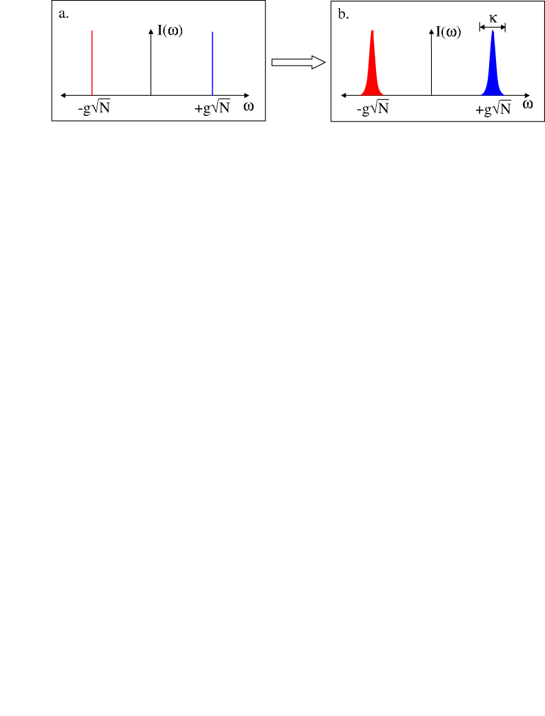
Figure 1: a. Intrinsic transmission spectrum of atoms-cavity system neglecting spatial dependence of potential and atomic motion. b. Transmission spectrum of spatially independent case including cavity decay.

Our treatment allows us to recover easily results of the Tavis-Cummings model tavis68 in which a collection of fixed two-level atoms are coupled to a single-mode cavity with fixed, identical dipole coupling. Considering $V(\mathbf{x_{0}})$ with all atoms at the origin ($\mathbf{x_{0}}=\left(0,0,\ldots 0\right)$), we find a spectrum composed of delta-functions at $\pm g\sqrt{N}$ (see Figure 1a) corresponding to the two bright states $\left|D_{\pm}(\mathbf{x_{0}})\right\rangle$. The clear dependence of the frequency of peak transmission on the integer number of atoms in the cavity provides the background for a basic, transmission-based atom-counting scheme. “Extrinsic” line-broadening, due to cavity decay and other losses, will smear out these sharp transmission peaks (see Figure 1b), and will determine the maximum number of atoms that can be counted at the single-atom level by discriminating between the transmission spectra for $N$ and $N+1$ atoms. For the remainder of the paper, we focus on intrinsic limitations to atom counting, i.e. those due to atomic localization and motion.

III Method of Moments

To analyze the transmission characteristics of the atoms-cavity system in the presence of spatial dependence and atomic motion, we shall assume that the key features of the spatially-independent limit discussed above are maintained (Figure 2). Specifically, the transmission spectrum will still be described by two sidebands, one red-shifted and one blue-shifted from the empty cavity resonance by some frequency on the order of $g$. In determining the cavity transmission $I(\omega)$, we may thus divide the bright excited states $\{\left|\Psi_{j}\right\rangle\}$ of the $n_{T}=1$ manifold into “red” $\{\left|\Psi_{j,-}\right\rangle\}$ and “blue” $\{\left|\Psi_{j,+}\right\rangle\}$ states. From these “red” and “blue” states, we determine the transmission lineshapes $I_{-}(\omega)$ and $I_{+}(\omega)$ of the red and blue sidebands, respectively.

The validity of this approach is made more exact by the following considerations. We have already obtained the locally-defined internal-state eigenbasis for the $n_{T}=1$ manifold as eigenstates of the operator $V(\mathbf{x})$, namely the states $\left|D_{\pm}(\mathbf{x})\right\rangle$ and the remaining $N-1$ dark states. Let $\hat{\mathcal{U}}(\mathbf{x})$ be the rotation operator which connects the uncoupled internal states $\{\left|0\right\rangle,\left|1\right\rangle,\dots\left|N\right\rangle\}$ to the eigenstates of $V(\mathbf{x})$ at a particular set of coordinates $\mathbf{x}$ (the “coupled internal state basis”). Now, consider applying this local choice of “gauge” everywhere in the system. Since the dipole interaction operator $V$ is diagonalized in the coupled internal state basis, it is convenient to examine the full Hamiltonian $H$ in this basis. Defining the spatially-dependent rotation operator $\hat{\mathcal{U}}=\int{d\mathbf{x}\,\left|\mathbf{x}\right\rangle\left\langle\mathbf{x}\right|\,\hat{\mathcal{U}}(\mathbf{x})}$, we therefore consider the transformed Hamiltonian $H^{\prime}=\hat{\mathcal{U}}H\hat{\mathcal{U}}^{\dagger}$.

Returning to Eq. (1), the only portion of the Hamiltonian $H$ which does not commute with the operator $\hat{\mathcal{U}}$ is the kinetic energy. Considering the transformation of the momentum operator for atom $i$,

$$\hat{\mathcal{U}}p_{i}\hat{\mathcal{U}}^{\dagger}=p_{i}+\frac{\hbar}{i}\hat{\mathcal{U}}\frac{d}{dx_{i}}\hat{\mathcal{U}}^{\dagger}=p_{i}+A_{i}$$ (7)

the transformed Hamiltonian $H^{\prime}$ can be expressed as $H^{\prime}=H_{ad}+\Delta H$, where

$$H_{ad} = \sum_{i}{\left(\frac{p_{i}^{2}}{2m}\otimes\mathcal{I}+\frac{1}{2}m\omega_{0}^{2}x_{i}^{2}\otimes\mathcal{I}\right)}+\hbar g\chi(\mathbf{x})\left(\left|D_{+}\right\rangle\left\langle D_{+}\right|-\left|D_{-}\right\rangle\left\langle D_{-}\right|\right),$$ (8)

$$\Delta H = \frac{1}{2m}\sum_{i}{\left(p_{i}A_{i}+A_{i}p_{i}+A_{i}A_{i}\right)}.$$ (9)

The operator $H_{ad}$ describes the behavior of atoms which adiabatically follow the coupled internal state basis while moving through the spatially-varying cavity field, and $\Delta H$ represents the kinetic energy associated with this local gauge definition.

Let us treat $\Delta H$ as a perturbation and expand the eigenvalues and eigenstates of $H^{\prime}$ as

$$E_{j,\pm} = E_{j,\pm}^{(0)}+E_{j,\pm}^{(1)}+\ldots,$$ (10)

$$\left|\Psi_{j,\pm}\right\rangle = \left|\Psi_{j,\pm}^{(0)}\right\rangle+\left|\Psi_{j,\pm}^{(1)}\right\rangle+\ldots$$ (11)

We define projection operators onto the red and blue and dark internal states, $\Pi_{-},\Pi_{+},\Pi_{d}$, respectively, with the explicit forms

$$\Pi_{\pm}=\int{d\mathbf{x}\left|\mathbf{x}\right\rangle\left\langle\mathbf{x}\right|\otimes\left|D_{\pm}(\mathbf{x})\right\rangle\left\langle D_{\pm}(\mathbf{x})\right|}.$$ (12)

These projection operators commute with $H_{ad}$. Hence the bright eigenstates of $H_{ad}$, which are simultaneous eigenstates of $\Pi_{\pm}$ and $\Pi_{d}$, can be written as

$$\left|\Psi_{j,\pm}^{(0)}\right\rangle=\left|\phi_{j,\pm}^{(0)}\otimes D_{\pm}\right\rangle\equiv\int{d\mathbf{x}\,\phi_{j,\pm}^{(0)}(\mathbf{x})\,\left|\mathbf{x}\right\rangle\otimes\left|D_{\pm}(\mathbf{x})\right\rangle}.$$ (13)

We now assign an eigenstate, $\left|\Psi_{j}\right\rangle$, of $H^{\prime}$ to the red or blue sideband if its zeroth order component $\left|\Psi_{j}^{(0)}\right\rangle$ belongs respectively to the $\left|D_{-}\right\rangle$ or $\left|D_{+}\right\rangle$ manifold. We can therefore define the sideband transmission spectra $I_{\pm}(\omega)$ as the separate contributions of red/blue sideband states to the total transmission spectra (see Eq. (2)):

$$I_{\pm}(\omega)\propto\sum_{j}{\left|\left\langle\Psi_{j,\pm}|\Psi_{I}\right\rangle\right|^{2}\delta(\omega_{j,\pm}-\omega_{0}-\omega)}.$$ (14)

Determining the exact form of $I_{\pm}(\omega)$ is equivalent to solving for all the eigenvalues $\hbar\omega_{j,\pm}$ of the full Hamiltonian. This is a difficult problem, particularly as the number of atoms in the cavity increases. In practice, given the potential extrinsic line-broadening effects which may preclude the resolution of individual spectral lines, it may suffice to simply characterize main features of the transmission spectra. As we show below, general expressions for the various moments of the spectral line can be obtained readily as a perturbation expansion in $\Delta H$. These moments allow one to assess the feasibility of precisely counting the number of atoms contained in the high-finesse cavity based on the transmission spectrum.

In general, we evaluate averages $\left\langle\omega_{\pm}^{n}\right\rangle$ weighted by the transmission spectral distributions $I_{\pm}(\omega)$. We make use of the straightforward identification (for notational clarity, shown here explicitly for the case of the blue sideband)

$$\hbar\left\langle\omega_{+}\right\rangle = \frac{\hbar\int{d\omega\,I_{+}(\omega)\,\omega}}{\int{d\omega\,I_{+}(\omega)}}$$ (15)

$$= \frac{\sum_{j}{E_{j,+}\left\langle\Psi_{I}|\Psi_{j,+}\right\rangle\left\langle\Psi_{j,+}|\Psi_{I}\right\rangle}}{\sum_{j}{\left\langle\Psi_{I}|\Psi_{j,+}\right\rangle\left\langle\Psi_{j,+}|\Psi_{I}\right\rangle}}$$ (16)

$$= \frac{\sum_{j}{E_{j,+}\left\langle\Psi_{I}\right|\left(\Pi_{+}+\Pi_{-}\right)\left|\Psi_{j,+}\right\rangle\left\langle\Psi_{j,+}\right|\left(\Pi_{+}+\Pi_{-}\right)\left|\Psi_{I}\right\rangle}}{\sum_{j}{\left\langle\Psi_{I}\right|\left(\Pi_{+}+\Pi_{-}\right)\left|\Psi_{j,+}\right\rangle\left\langle\Psi_{j,+}\right|\left(\Pi_{+}+\Pi_{-}\right)\left|\Psi_{I}\right\rangle}},$$ (17)

where we have made use of the facts that $\Pi_{+}+\Pi_{-}+\Pi_{d}=I$ and $\Pi_{d}\left|\Psi_{I}\right\rangle=0$. To zeroth order, Eq. (15) becomes,

$$\hbar\left\langle\omega_{+}\right\rangle^{(0)} = \frac{\sum_{j}{E_{j,+}^{(0)}\left\langle\Psi_{I}|\Psi_{j,+}^{(0)}\right\rangle\left\langle\Psi_{j,+}^{(0)}|\Psi_{I}\right\rangle}}{\sum_{j}{\left\langle\Psi_{I}|\Psi_{j,+}^{(0)}\right\rangle\left\langle\Psi_{j,+}^{(0)}|\Psi_{I}\right\rangle}}=2\left\langle\Psi_{I}\right|{\Pi_{+}}H_{ad}{\Pi_{+}}\left|\Psi_{I}\right\rangle.$$ (18)

The first-order correction to this result is given by,

$$\begin{array}[]{rcl}\hbar\left\langle\omega_{+}\right\rangle^{(1)}&=&2\left(\left\langle\Psi_{I}\right|\Pi_{+}\Delta H\Pi_{+}\left|\Psi_{I}\right\rangle+\left\langle\Psi_{I}\right|\Pi_{-}\sum_{j}{E_{j,+}^{(0)}\left|\Psi_{j,+}^{(1)}\right\rangle\left\langle\Psi_{j,+}^{(0)}\right|}\Pi_{+}\left|\Psi_{I}\right\rangle+\left\langle\Psi_{I}\right|\Pi_{+}\sum_{j}{E_{j,+}^{(0)}\left|\Psi_{j,+}^{(0)}\right\rangle\left\langle\Psi_{j,+}^{(1)}\right|}\Pi_{-}\left|\Psi_{I}\right\rangle\right)\\ &&-4\left\langle\Psi_{I}\right|\Pi_{+}H_{ad}\Pi_{+}\left|\Psi_{I}\right\rangle\left(\left\langle\Psi_{I}\right|\Pi_{-}\sum_{j}{\left|\Psi_{j,+}^{(1)}\right\rangle\left\langle\Psi_{j,+}^{(0)}\right|}\Pi_{+}\left|\Psi_{I}\right\rangle+\left\langle\Psi_{I}\right|\Pi_{+}\sum_{j}{\left|\Psi_{j,+}^{(0)}\right\rangle\left\langle\Psi_{j,+}^{(1)}\right|}\Pi_{-}\left|\Psi_{I}\right\rangle\right).\end{array}$$ (19)

To evaluate the sums over the first-order corrections to the eigenstates, $\left|\Psi_{j,\pm}^{(1)}\right\rangle$, we approximate the energy denominator in the first-order perturbation correction as the difference between the average energies of the red and blue sidebands,

$$\left\langle\Psi_{I}\right|\Pi_{-}\sum_{j}{\left|\Psi_{j,+}^{(1)}\right\rangle\left\langle\Psi_{j,+}^{(0)}\right|}\Pi_{+}\left|\Psi_{I}\right\rangle = \left\langle\Psi_{I}\right|\sum_{j}{\sum_{k}{\frac{\left|\Psi_{k,-}^{(0)}\right\rangle\left\langle\Psi_{k,-}^{(0)}\right|\Delta H\left|\Psi_{j,+}^{(0)}\right\rangle}{\hbar\omega_{j,+}^{(0)}-\hbar\omega_{k,-}^{(0)}}\left\langle\Psi_{j,+}^{(0)}\right|}}\Pi_{+}\left|\Psi_{I}\right\rangle,$$ (20)

$$\approx \frac{1}{\left\langle\hbar\omega_{+}^{(0)}\right\rangle-\left\langle\hbar\omega_{-}^{(0)}\right\rangle}\left\langle\Psi_{I}\right|\Pi_{-}\Delta H\Pi_{+}\left|\Psi_{I}\right\rangle.$$ (21)

Using this approximation, we can evaluate Eq. (15) to the first order in perturbation, yielding

$$\begin{array}[]{ll}\hbar\left\langle\omega_{+}\right\rangle=&2\left\langle\Pi_{+}H\Pi_{+}\right\rangle+\frac{1}{\left\langle\hbar\omega_{+}^{(0)}\right\rangle-\left\langle\hbar\omega_{-}^{(0)}\right\rangle}\bigl{(}4\left\langle\Pi_{+}H_{ad}\Delta H\Pi_{-}\right\rangle-8\left\langle\Pi_{+}H_{ad}\Pi_{+}\right\rangle\left\langle\Pi_{-}\Delta H\Pi_{+}\right\rangle\bigr{)},\end{array}$$ (22)

where all expectation values are calculated over the initial state $\left|\Psi_{I}\right\rangle$. We can also calculate the second moment of the distribution using the same technique. To first-order, we obtain,

$$\begin{array}[]{ll}\hbar^{2}\left\langle\omega_{+}^{2}\right\rangle=&2\left\langle\Pi_{+}\left(H_{ad}^{2}+\Delta HH_{ad}+H_{ad}\Delta H\right)\Pi_{+}\right\rangle+\frac{1}{\left\langle\hbar\omega_{+}^{(0)}\right\rangle-\left\langle\hbar\omega_{-}^{(0)}\right\rangle}\bigl{(}4\left\langle\Pi_{+}H_{ad}^{2}\Delta H\Pi_{-}\right\rangle\\ &-8\left\langle\Pi_{+}H_{ad}^{2}\Pi_{+}\right\rangle\left\langle\Pi_{-}\Delta H\Pi_{+}\right\rangle\bigr{)}.\end{array}$$ (23)

In order to evaluate these expressions, we must calculate expectation values of the form $\Pi^{\pm}H_{ad}^{j}\Delta H^{k}\Pi^{\pm}$ over the initial state $\left|\Psi_{I}\right\rangle$. To simplify matters, we note that we can act with the projection operators on the initial state $\left|\Psi_{I}\right\rangle$, which is equivalent to operating in the $\left|D_{\pm}\right\rangle$ internal state basis. Since $H_{ad}$ is diagonal in the $\left|D_{\pm}\right\rangle$ basis, and $\phi_{I}(\mathbf{x})$ is the $N$-dimensional harmonic oscillator ground state, it is straightforward to obtain

$$H_{ad}\left|\phi_{I}(\mathbf{x})D_{\pm}\right\rangle=\left(E_{0}+\hbar g\chi(\mathbf{x})\right)\left|\phi_{I}(\mathbf{x})D_{\pm}\right\rangle.$$ (24)

Using the definition in Eq. (9), we find that the $\left|D_{\pm}\right\rangle$ matrix elements of $\Delta H$ are given by the matrix

$$\Delta H=\frac{\hbar^{2}k^{2}\zeta(\mathbf{x})}{4m}\otimes\left(\begin{array}[]{cc}1&-1\\ -1&1\end{array}\right),$$ (25)

where we have defined,

$$\zeta(\mathbf{x})=-\frac{N-1}{\chi^{2}}+1-\sum_{i=1}^{N}{\frac{\cos^{4}{(kx_{i})}}{\chi^{4}}}.$$ (26)

Combining Eqs. (22) and (23) with Eqs. (24) and (25), we obtain to first-order in $\Delta H$,

$$\hbar\left\langle\omega_{+}\right\rangle-E_{0} = \hbar g\left\langle\chi\right\rangle+\frac{1}{2}\frac{\hbar^{2}k^{2}}{2m}\left\langle\zeta\right\rangle+\frac{1}{2}\frac{\hbar^{2}k^{2}}{2m}\frac{1}{\left\langle\chi\right\rangle}\left(-\left\langle\zeta\chi\right\rangle+\left\langle\zeta\right\rangle\left\langle\chi\right\rangle\right),$$ (27)

$$\hbar^{2}\left(\left\langle\omega_{+}^{2}\right\rangle-\left\langle\omega_{+}\right\rangle^{2}\right) = \hbar^{2}g^{2}\left(\left\langle\chi^{2}\right\rangle-\left\langle\chi\right\rangle^{2}\right)+\hbar g\frac{\hbar^{2}k^{2}}{2m}\left(\frac{1}{\left\langle\chi\right\rangle}\left(\left\langle\zeta\chi^{2}\right\rangle+\left\langle\zeta\right\rangle\left\langle\chi^{2}\right\rangle\right)-2\left\langle\zeta\right\rangle\left\langle\chi\right\rangle\right).$$ (28)

Here all expectation values are taken over the spatial state $\phi_{I}(\mathbf{x})$. Although the function $\phi_{I}(\mathbf{x})$ is simply the product of $N$ harmonic oscillator ground states, the presence of various powers of $\chi(\mathbf{x})$ and $\zeta(\mathbf{x})$ in the above expectation values makes their analytic evaluation very difficult for arbitrary $N$.To determine the dependence of these integrals on atom number $N$, one may expand the integrand as a Taylor series in $\chi^{2}$, leading to approximate analytic solutions for the integral as a series in $1/N$. After some tedious algebra, we find the average positions of the red- and blue-transmission sidebands to be

$$\begin{array}[]{rcl}\hbar\left\langle\omega_{\pm}\right\rangle-E_{0}&=&\pm\hbar g\sqrt{N}\sqrt{\frac{1+\epsilon}{2}}\left(1-\frac{1}{N}\frac{(1-\epsilon)^{2}}{16}\right)-\frac{\hbar^{2}k^{2}}{2m}\left(\frac{1-\epsilon}{2(1+\epsilon)}\right)+O\left(\frac{1}{N}\right).\end{array}$$ (29)

Here we quantify the relative length scales of the initial harmonic trap as compared to the optical interaction potential through the parameter $\epsilon=\exp{\left(-k^{2}\sigma^{2}\right)}$, which is related to the Lamb-Dicke parameter $\eta$ by $\sqrt{2}\eta=k\sigma$ and $\sigma=\sqrt{\hbar/m\omega_{0}}$.

Next, we obtain an expression for the width of the red and blue sidebands by evaluating the second moment of the sidebands. Expanding Eq. (28) as a series in $1/N$, we obtain

$$\begin{array}[]{rcl}\hbar^{2}\left(\left\langle\omega^{2}_{\pm}\right\rangle-\left\langle\omega_{\pm}\right\rangle^{2}\right)&=&\frac{1}{16}\hbar^{2}g^{2}\left(1-\epsilon\right)^{2}\left(1+\epsilon\right)\pm\hbar g\frac{\hbar^{2}k^{2}}{2m}\frac{1}{4\sqrt{N}\sqrt{2\left(1+\epsilon\right)}}\left(1-\epsilon\right)^{2}\left(3+\epsilon\right)+O\left(\frac{1}{N}\right).\end{array}$$ (30)

To gain some physical insight into these results, we consider two important regimes: the tight and loose trap regimes. These different regimes are reflected in the corresponding values of the parameter $\epsilon$, which tends towards $1$ in the extreme tight-trap limit and to $0$ in the extreme loose-trap limit. In the tight regime, the length scale of the trapping potential is much smaller than the wavelength of the light, i.e. $k\sigma\ll 1$. This is equivalent to the Lamb-Dicke regime and is applicable to current experiments for trapped ions in cavities guth02ion ; mundt02 , or for neutral atoms held in deep optical potentials ye99trap . In the loose-trap regime, $k\sigma\geq 1$ and atoms in the ground state of the harmonic oscillator potential are spread out over a distance comparable to the optical wavelength. As atoms in this regime sample broadly the cavity field, one expects, and indeed finds, a significant inhomogeneous broadening of the atoms-cavity resonance.

In the extreme loose-trap limit ($\epsilon\to 0$), we find

$$\left\langle\omega_{\pm}\right\rangle-E_{0}/\hbar = \pm g\sqrt{\frac{N}{2}}\left(1-\frac{1}{16N}\right)+\frac{1}{2}\frac{\hbar k^{2}}{2m}+O\left(\frac{1}{N}\right),$$ (31)

$$\left\langle(\Delta\omega_{\pm})^{2}\right\rangle = \frac{1}{8}g^{2}\pm g\frac{\hbar k^{2}}{2m}\frac{3}{4\sqrt{2N}}+O\left(\frac{1}{N}\right).$$ (32)

In the loose-trap limit, the center of the red sideband is now located at $g\sqrt{N/2}$ instead of at $g\sqrt{N}$ as we obtained for the spatially independent case. This difference is due to the spatial dependence of the standing mode; the atoms no longer always feel the full strength of the potential, but are sometimes located at nodes of the potential. We also see that the sidebands have an intrinsic width of $\approx g/\sqrt{8}$. This width will play an important part in limiting our ability to count the number of atoms in the cavity in the limit of a loose trap.

Considering the tight-trap limit, we expand in the small parameter $k\sigma$ and obtain

$$\left\langle\omega_{\pm}\right\rangle-E_{0}/\hbar = \pm g\sqrt{N}\left(1-\frac{1}{4}k^{2}\sigma^{2}\right)-\frac{1}{4}\frac{\hbar k^{2}}{2m}k^{2}\sigma^{2}+O\left(k^{4}\sigma^{4}\right),$$ (33)

$$\left\langle(\Delta\omega_{\pm})^{2}\right\rangle = \frac{1}{8}g^{2}k^{4}\sigma^{4}\pm g\frac{\hbar k^{2}}{2m}\frac{1}{2\sqrt{N}}k^{4}\sigma^{4}+O\left(k^{6}\sigma^{6}\right).$$ (34)

In the limit $k\sigma\to 0$, the atoms are confined to the origin and we recover the Tavis-Cummings result discussed earlier, wherein the transmission sidebands are delta functions at $\pm g\sqrt{N}$ away from the empty cavity resonance. As the tightness of the trap decreases, the atoms begin to expericence the weaker regions of the optical potential and the centers of the sidebands move towards the origin. In addition, the sidebands develop an intrinsic variance which scales as $k^{4}\sigma^{4}$.

An important feature of both regimes is the intrinsic linewidth of both the red and blue sidebands (see Figure 2a). This linewidth has a magnitude of approximately $g\sqrt{(1-\epsilon)/8}$ when the vacuum Rabi splitting is much larger than the atomic recoil energy, i.e., $g\gg\hbar k^{2}/2m$. It is unrelated to linewidth due to cavity decay or spontaneous emission which we have not addressed here and results purely from the spatial dependence of the atom-cavity coupling. Thus, it will provide an intrinsic limit to our ability to count $N$ atoms, regardless of the quality of the cavity that is used. Our expression for the intrinsic linewidth also highlights an asymmetry between the red and blue sidebands. To first-order, increasing the atomic recoil energy reduces the linewidth of the red sideband but increases the linewidth of the blue sideband. Consequently probing the red sideband of the atoms-cavity system rather than the blue sideband would facilitate counting atoms. In addition, these results suggest that the ability to tune both the atomic recoil energy $\hbar k^{2}/2m$ and the coupling strength $g$ (this can be done, for instance, using CQED on Raman transitions) would be beneficial. We attribute the asymmetry between the sidebands to the different effective potentials seen by states within the red and blue sidebands. A detailed analysis of this aspect will be provided in a future publication.

IV Conclusions

We have found that the transmission spectrum of the cavity containing $N$ atoms trapped initially in the ground state of an harmonic potential will consist of distinct transmission sidebands which are red- and blue-detuned from the bare-cavity resonance, when the vacuum Rabi splitting dominates the atomic recoil energy. Analytic expressions for the first and second moments of the transmission sidebands were derived, and evaluated in the limits of tight and loose initial confinement. These expressions include terms containing the vacuum Rabi splitting $\hbar g$ and the recoil energy $\hbar^{2}k^{2}/2m$. The former can be regarded as line shifts and broadenings obtained by quantifying inhomogeneous broadening under a local-density approximation, i.e. treating the initial atomic state as a statistical distribution of infinitely massive atoms. The latter quantifies residual effects of atomic motion, in essence quantifying effects of Doppler shifts and line broadenings.

These results can be applied to assess the potential for precisely counting the number of atoms trapped in a high-finesse optical cavity through measuring the transmission of probe light, analogous to the work of Hood et al. hood00micro and Münstermann et al. hood00micro ; munst99dyn for single atom detection. To set the limits of our counting capability, we assume that atoms are detected through measuring the position of the mean of the red sideband. In order to reliably distinguish between $N$ and $N+1$ atoms in the cavity, the difference between the means for $N$ and $N+1$ atoms must be greater than the width of our peaks, i.e., $\left|\left\langle\omega_{\pm}(N)\right\rangle-\left\langle\omega_{\pm}(N+1)\right\rangle\right|>\Delta\omega_{\pm}$ (see Figure 3). Let us consider that, in addition to the intrinsic broadening derived in this paper, there exists an extrinsic width $\kappa^{\prime}$ due to the finite cavity finesse and other broadening mechanisms. Evaluated in the limit $g\gg\hbar k^{2}/2m$ and assuming large $N$,

$$\left\langle\omega_{-}(N)\right\rangle-\left\langle\omega_{-}(N+1)\right\rangle\simeq g\sqrt{\frac{1+\epsilon}{8N}}.$$ (35)

We thus obtain an atom counting limit of

$$N_{max}\simeq\frac{1+\epsilon}{8\frac{\kappa^{\prime\,2}}{g^{2}}+\frac{1}{2}(1-\epsilon)^{2}(1+\epsilon)}.$$ (36)

where we have assumed that the intrinsic and extrinsic widths add in quadrature. This atom counting limit ranges from $N_{max}=g^{2}/4\kappa^{\prime\,2}$ in the tight-trap limit, to $N_{max}=1/(1/2+8\kappa^{\prime\,2}/g^{2})$ in the loose trap limit. Figure 4 shows $N_{max}$ as a function of $\epsilon$ for various values of $\kappa$. In general, atom counting will be limited by extrinsic linewidth when $16\kappa^{\prime 2}>g^{2}(1-\epsilon)^{2}$ and by intrinsic linewidth when $16\kappa^{\prime 2}<g^{2}(1-\epsilon)^{2}$.

These results demonstrate that atom counting using the transmission spectrum is best accomplished within the tight-trap limit. Certainly, in the loose-trap limit, atom counting will be rendered difficult as the intrinsic linewidth of the sidebands is increased. However, several questions regarding the feasibility of atom counting experiments remain. First, although atom counting by a straightforward measurement of the intensity of the transmitted light may be difficult, it is possible that the phase of the transmitted light may be less affected by motional effects mabuchi99single . Dynamical measurements (possibly using quantum feedback techniques) might also yield higher counting limits. Second, atomic cooling techniques could be used in the loose-trap limit to cool the atoms into the wells of the optical potential, thereby decreasing the observed linewidth vul ; hech ; van . Finally, the state-dependence of spontaneous emission has not yet been taken into account. Although the loose-trap regime leads to an intrinsic linewidth which limits atom counting, it may also suppress the extrinsic linewidth as a result of contributions from superluminescence. On the other hand, in the Lamb-Dicke limit, the atoms are all highly localized, which could lead to enhanced spontaneous emission due to cooperative effects. Future work will investigate alternative methods of atom counting and will explore complementary techniques of reducing the intrinsic linewidth in atom-cavity transmission spectra.

Figure 2: a. Intrinsic transmission spectrum of atoms-cavity system including spatial dependence of potential and atomic motion. b. Corresponding transmission spectrum including cavity decay.

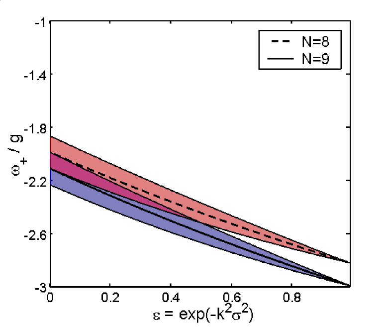
Figure 3: Plot of $\left\langle\omega_{-}\right\rangle$ as a function of the trap tightness $\epsilon=\exp{(-k^{2}\sigma^{2})}$ for $N=8$ and $N=9$ and small ratio of atomic recoil energy to vacuum Rabi splitting, $\hbar k^{2}/2mg=0.01$. The shaded regions indicate the instrinsic width of the red sideband, $\pm\sqrt{\left\langle(\Delta\omega_{-})^{2}\right\rangle}/2$. In the tight-trap limit, $N=8$ and $N=9$ can be distinguished. In the loose-trap limit, the intrinsic width of the spectra render determination of atom number difficult.

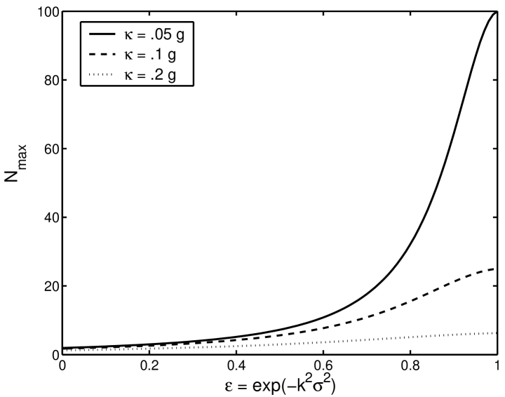
Figure 4: Maximum limit $N_{max}$ on atom counting as a function of trap tightness $\epsilon=\exp{(-k^{2}\sigma^{2})}$ for several values of the decay parameter $\kappa$. $\epsilon\to 0$ corresponds to the loose-trap limit while $\epsilon\to 1$ corresponds to the tight-trap limit. Notice that for the infinitely tight trap, atom counting is limited only by $\kappa$.

References

- (1) Cavity quantum electrodynamics, edited by P. Berman (Academic Press, Boston, 1994).
- (2) H. Kimble, Physica Scripta T76, 127 (1998).
- (3) J. Raimond, M. Brune, and S. Haroche, Reviews of Modern Physics 73, 565 (2001).
- (4) C. Law and H. Kimble, Journal of Modern Optics 44, 2067 (1997).
- (5) A. Kuhn et al., App. Phys. B B69, 373 (1997).
- (6) A. Kuhn, M. Hennrich, and G. Rempe, Phys. Rev. Lett. 89, 067901 (2002).
- (7) K.R. Brown et al., Phys. Rev. A 67, (2003).
- (8) Q. Turchette et al., Phys. Rev. Lett. 75, 4710 (1995).
- (9) G. Guthohrlein et al., Nature 414, 49 (2002).
- (10) A. Mundt et al., Phys. Rev. Lett. 89, 103001 (2002).
- (11) C. Hood et al., Science 287, 1447 (2000).
- (12) P. Münstermann et al., Phys. Rev. Lett. 82, 3791 (1999).
- (13) H. Mabuchi, J. Ye, and H. Kimble, App. Phys. B 68, 1095 (1999).
- (14) P. Horak et al., Phys. Rev. Lett. 88, 043601 (2002).
- (15) C. Orzel et al., Science 291, 2386 (2001).
- (16) D. Wineland et al., Phys. Rev. A 46, R6797 (1992).
- (17) J. Hald et al., Phys. Rev. Lett. 83, 1319 (2000).
- (18) A. Kuzmich, L. Mandel, and N.P. Bigelow, Phys. Rev. Lett. 85, 1594 (2000).
- (19) J. Ye, D.W. Vernooy, and H.J. Kimble, Phys. Rev. Lett. 83, 4987 (1999).
- (20) J. McKeever et al., Phys. Rev. Lett. 90, 133602 (2003).
- (21) M. Tavis and F. Cummings, Phys. Rev. 170, 379 (1968).
- (22) W. Ren and H.J. Carmichael, Phys. Rev. A 51, 752 (1995).
- (23) D.W. Vernooy and H.J. Kimble, Phys. Rev. A 56, 4287 (1997).
- (24) A. Doherty et al., Phys. Rev. A 56, 833 (1997).
- (25) V. Vuletic and S.Chu, Phys. Rev. Lett. 84, 3787 (2000).
- (26) G. Hechenblaikner, M. Gangl, P. Horak, H. Ritsch, Phys. Rev. A 58, 3030 (1998).
- (27) S.J. van Enk, J. McKeever, H.J. Kimble, J. Ye, Phys. Rev. A 64, 013407 (2001).