Quantum adiabatic algorithm for Hilbert’s tenth problem:
I. The algorithm

Abstract

We review the proposal of a quantum algorithm for Hilbert’s tenth problem and provide further arguments towards the proof that: (i) the algorithm terminates after a finite time for any input of Diophantine equation; (ii) the final ground state which contains the answer for the Diophantine equation can be identified as the component state having better-than-even probability to be found by measurement at the end time–even though probability for the final ground state in a quantum adiabatic process need not monotonically increase towards one in general. Presented finally are the reasons why our algorithm is outside the jurisdiction of no-go arguments previously employed to show that Hilbert’s tenth problem is recursively non-computable.

I Introduction

We have claimed Kieu (2003a, b, d, c) to have a quantum algorithm for Hilbert’s tenth problem Matiyasevich (1993) despite the fact that the problem has been proved to be recursively noncomputable. The algorithm makes essential use of the Quantum Adiabatic Theorem (QAT) Messiah (1999) and other results (to be further substantiated in this paper) in the framework of Quantum Adiabatic Computation Farhi et al. (2000) in order to provide a single, universal procedure, physical or otherwise, which consumes finite amount of resources and terminates in a finite time and which can tell, in principle, whether any given Diophantine equation  has any non-negative integer solution or not–thus solving Hilbert’s tenth.

We refer the readers to the above references and elsewhere for the history of Hilbert’s tenth problem and its paramount importance in Mathematics and Theoretical Computer Science, as well as in Philosophy. In the next Section, we summarise the algorithm which employs Quantum Adiabatic Processes (QAP). Following that, we provide some arguments asserting why there is no level crossing, as required by the QAT, in the spectral flow associated with the QAP, except possibly at the end points. This will ensure that our algorithm can terminate in a finite time duration which is dictated by the smallest, non-vanishing energy gap separating the instantaneous ground state and relevant excited state in the spectral flow. We next provide the proof for the criterion identifying the final ground state of two-state systems, and then argue that this criterion is also generalisable to systems of infinitely many states of our algorithm. We also consider the algorithm in the context of existing no-go arguments for Hilbert’s tenth problem in order to point out that the algorithm is outside the jurisdiction of those arguments. The paper is concluded with some remarks.

II The Quantum Adiabatic Algorithm

II.1 Statement of the algorithm

We first introduce the occupation-number state $|n\rangle$, $n=0,1,2,\ldots$, and the creation and annihilation operators $a^{\dagger}$ and $a$ respectively

$$a|0\rangle = 0,$$

$$a|n\rangle = \sqrt{n}|n-1\rangle,$$

$$a^{\dagger}|n\rangle = \sqrt{n+1}|n+1\rangle,$$

$$(a^{\dagger}a)|n\rangle = n|n\rangle,$$ (1)

and the coherent state, with complex number $\alpha$,

$$|\alpha\rangle = e^{-\frac{|\alpha|^{2}}{2}}\sum_{n=0}^{\infty}\frac{\alpha^{n}}{\sqrt{n!}}|n\rangle.$$ (2)

Now, given a Diophantine equation with $K$ unknowns,

$$D(x_{1},\ldots,x_{K})=0,$$ (3)

we provide the following quantum algorithm to decide whether this equation has any non-negative integer solution or not:

1. Construct/simulate a physical process in which a system initially starts with a direct product of $K$ coherent states

   $$|\psi(0)\rangle = |\{\alpha\}_{I}\rangle\equiv\bigotimes_{i=1}^{K}|\alpha_{i}\rangle,$$ (4)

   and in which the system is subject to a time-dependent Hamiltonian over the time interval $[0,T]$, for some time $T$,

   $${\cal H}(t) \equiv \left(1-\frac{t}{T}\right)H_{I}+\frac{t}{T}H_{P},$$ (5)

   with the initial Hamiltonian

   $$H_{I} = \sum_{i=1}^{K}\left(a_{i}^{\dagger}-\alpha^{*}_{i}\right)\left(a_{i}-\alpha_{i}\right),$$ (6)

   and the final Hamiltonian

   $$H_{P} = \left(D(a^{\dagger}_{1}a_{1},\ldots,a^{\dagger}_{K}a_{K})\right)^{2}.$$ (7)

2. Measure/calculate (through the Schrödinger equation with the time-dependent Hamiltonian above) the maximum probability to find the system in a particular occupation-number state at the chosen time $T$,

   $$P(T) = \max_{|\{n\}\rangle}|\langle\psi(T)|\{n\}\rangle|^{2},$$ (8)

   $$= \left|\langle\psi(T)|\{n\}_{0}\rangle\right|^{2},$$

   where $|\{n\}_{0}\rangle$ (which is a direct product of $K$ particular occupation-number states, $\bigotimes_{i=1}^{K}|n_{i}^{0}\rangle$) provides that maximal probability among all other direct products of $K$ occupation-number states.

3. If $P(T)\leq 1/2$, increase $T$ and repeat all the steps above.

4. If $P(T)>1/2$, then $|\{n\}_{0}\rangle$ is the ground state of $H_{P}$ (assuming no degeneracy–we discuss the case of degeneracy below) and we can terminate the algorithm and deduce a conclusion from the fact that:

   $$H_{P}|\{n\}_{0}\rangle=0{\mbox{ {\bf iff} the equation~{}(\ref{equation}) has a non-negative integer solution.}}$$ (9)

We refer to Kieu (2003a, b, d) for the motivations and discussions leading to the algorithm above. Note that it is crucial that $H_{I}$ does not commute with $H_{P}$,

$$[H_{I},H_{P}] \not= 0,$$ (10)

and of course both Hamiltonians are of infinite dimensions. (This condition can be relaxed to that of unbounded dimensions, see later.)

To remove any possible degeneracy of the ground state for any $H_{P}$, we can always introduce to $H_{P}$ a symmetry-breaking term of the form $(\gamma a^{\dagger}_{i}+\gamma^{*}a_{i})$ for some $i$ in the limit ${|\gamma|}\to 0$ Kieu (2003d). This term destroys the symmetry generated from the commutation between $H_{P}$ and the occupation-number operators. However, we can always recover the symmetry in the limit and modify the algorithm above slightly to reach an answer for the Diophantine equation in question. Note also that the arguments of the Section III below can be easily modified to accommodate this symmetry-breaking term to ensure there is no ground-state degeneracy in $0\leq t/T<1$.

II.2 Its probabilistic nature

We will prove in the next Section that there exists a finite $T$ whence the algorithm can be terminated. But it is important to recognise hereby that our algorithm is probabilistic in nature. As the halting criterion, the probability $P(T)$ of (8) for certain state need to be more than one-half. If the algorithm is implemented by certain physical process then we can approximate this probability by the relative frequency that a particular state is obtained in repeating the measurements many times over. The Weak Law of Large Numbers, however, can only assert that this frequency is within a distance $\epsilon$ of $P(T)$ with certain probability of at least $1-\delta$. It is this probability $1-\delta$ that gives the quantum algorithm its probabilistic nature. Both $\epsilon$ and $\delta$ are dependent on the number of measurement repetitions from which the frequency is obtained–see, for example, Rozanov (1977) for a statement and proof of the theorem. In general, we can always reduce $\epsilon$ and $\delta$ to arbitrarily close to zero by increasing the number of repetitions $L$ appropriately,

$$L>1/(4\epsilon^{2}\delta).$$ (11)

As an anticipation of the numerical simulations of the algorithm on recursive computers Kieu (2003c, e), we mention now that the probabilistic nature of the algorithm is manifest differently there through the extrapolation to zero step size in solving the Schrödinger equation. Such extrapolation is necessary for a correct truncation, for a given Diophantine equation, of the dimensions of the Hilbert space involved.

We will later come back to this probabilistic nature in Section V in the discussion of no-go arguments for Hilbert’s tenth problem. In ending this Section, we wish to point out here that, contrary to common misunderstanding, probabilistic computation in general is not equivalent in terms of computability to Turing computation Ord and Kieu (2003a).

III No level crossing for the ground state

One of the sufficient conditions for the Quantum Adiabatic Theorem Messiah (1999) is that the relevant level, which in our case is the instantaneous ground state, doesnot cross with any other level as time progresses. In Kieu (2003d) we have given some arguments for no level crossing for the time-dependent Hamiltonian

$${\cal H}(sT) = (1-s)H_{I}+sH_{P},$$ (12)

with the reduced time $s$ in the interval $s\in(0,1)$. Now we present below some other arguments adapted from those of Ruskai Ruskai (2002), which in turn are based on Perron-Frobenius’s theorem Horn and Johnson (1985) for finite but unbounded number of dimensions, and on Reed-Simon’s theorems Reed and Simon (1978) for infinite number of dimensions.

Let us consider the exponential operator $\exp(-{\cal H}(sT))$, it can be expressed by the Lie-Trotter product formula as

$${e}^{-{\cal H}(sT)} = \lim_{M\to\infty}\left({e}^{-\frac{s}{M}H_{P}-\frac{1-s}{M}\sum_{i}(a^{\dagger}_{i}a_{i}+\alpha^{*}_{i}\alpha_{i})}\left[{e}^{\frac{1-s}{M}\sum_{i}\alpha_{i}a^{\dagger}_{i}}{e}^{\frac{1-s}{M}\sum_{i}\alpha^{*}_{i}a_{i}}\right]\right)^{M}.$$ (13)

For general operators in dimensionally infinite Hilbert spaces, the convergence in the above is understood to be the strong convergence of the rhs to the lhs .

III.1 Finite but unbounded number of dimensions

Our algorithm of the last Section actually requires only sufficiently large but finite Hilbert space with a truncated basis consisting of occupation-number vectors, $\{|n\rangle:n=0,1,\ldots,N\}$, for some $N$ beyond which higher occupation-number states contribute negligibly to the dynamics of low-lying states relevant to our problem. This follows from the facts that the normalised wavefunction at any given time has a support which spreads significantly only over a finite range of occupation-number states, and that the explicit coupling, and thus the influence, between one particular instantaneous eigenstate and other diminishes significantly outside some finite range of occupation-number states (as can be seen through a set of differential equations in Kieu (2003d) connecting instantaneous eigenstates of ${\cal H}(t)$ at different time $t$). We will exploit these facts fully in the numerical simulations of the quantum algorithm Kieu (2003c, e). How large is sufficient, and thus how much the truncation $N$ should be, depend very much on the particular Diophantine equation being investigated. Such truncation will be discussed and implemented in the numerical ssimulations of the quantum algorithm Kieu (2003c, e). In the last Section, we need not worry about the size of $N$ as we have employed dimensionally infinite Hilbert space. However, for any arbitrary and unbounded $N$, the Hamiltonian (12) above has a representation which is a finite square matrix and in which all the off-diagonal elements are contained in $H_{I}$.

The elements of the matrix product in the square brackets on the rhs of (13), can be expressed in the truncation to an arbitrary $N$ (where $a^{\dagger}|N\rangle=0$) as

$$\langle m|{e}^{\beta_{i}a^{\dagger}_{i}}{e}^{\beta^{*}_{i}a_{i}}|n\rangle = \sum_{q=0}^{N}\langle m|{e}^{\beta_{i}a^{\dagger}_{i}}|q\rangle\langle q|{e}^{\beta^{*}_{i}a_{i}}|n\rangle,$$ (14)

$$= \sum_{q=0}^{N}\langle m|\sum_{k=0}^{\infty}\frac{(\beta_{i}a^{\dagger}_{i})^{k}}{k!}|q\rangle\langle q|\sum_{l=0}^{\infty}\frac{(\beta_{i}^{*}a_{i})^{l}}{l!}|n\rangle,$$

where

$$\beta_{i}=\frac{1-s}{M}\alpha_{i}.$$ (15)

It then follows that for $\{\alpha_{i}\}$ real and positive, and for $0\leq s<1$, the lhs above is always non-zero and positive. For example, when $N>m>n$, at least the term with $k=m-n$ and $l=0$ will contribute nonvanishingly and positively to the sum of non-negative terms on the rhs to ensure the matrix element on the lhs is always positive.

In the basis of occupation-number states, the first factor in the bracket of the rhs of (13) is a diagonal matrix, whose net effect is to multiply each row of the matrix product in square brackets in (13) by non-zero, positive numbers (being exponentials). As a result, for $\alpha_{i}=\alpha_{i}^{*}>0,{\mbox{ for }}i=1,2,\ldots,K$, the product in the bracket on the rhs of (13) has only positive elements, and so has its $m$-th power. Thus, Perron-Frobenius’s theorem Horn and Johnson (1985) for (finite) matrices with strictly positive elements can be applied to the lhs of (13) to confirm that the largest eigenvector of ${\rm e}^{-{\cal H}(sT)}$ is unique for these values of $\{\alpha_{i}\}$. That is, ${\cal H}(sT)$ itself has a unique ground state for $0\leq s<1$ (since, by construction, ${\cal H}(0)=H_{I}$ has a nondegenerate ground state).

At $s=1$, the matrix ${\rm e}^{-\frac{1-s}{M}H_{I}}$ becomes the identity matrix which has zero non-diagonal elements and becomes reducible, violating the conditions of Perron-Frobenius’s theorem and thus allowing the possibility that ${\cal H}(T)=H_{P}$ has a degenerate ground state.

III.2 Infinite number of dimensions

To handle the infinite dimensions of the operator product in the square brackets of (13) directly, that is, without any truncation, we can employ the so-called holomorphic representation Faddeev and Slavnov (1980); Itzykson and Zuber (1980) to arrive at

$$\langle m|{e}^{\beta_{i}a^{\dagger}_{i}}{e}^{\beta^{*}_{i}a_{i}}|n\rangle = \int\frac{d\bar{\eta}d\eta}{2\pi i}\frac{d\bar{\omega}d\omega}{2\pi i}\frac{d\bar{\xi}d\xi}{2\pi i}\frac{\eta^{m}}{\sqrt{m!}}e^{-\bar{\eta}\eta}e^{\bar{\eta}\omega+\bar{\eta}\beta_{i}}e^{-\bar{\omega}\omega}e^{\bar{\omega}\xi+\beta_{i}^{*}\xi}e^{-\bar{\xi}\xi}\frac{\bar{\xi}^{n}}{\sqrt{n!}},$$ (16)

$$= \frac{1}{\sqrt{m!n!}}\left(\frac{\partial}{\partial\bar{s}}\right)^{m}\left(\frac{\partial}{\partial s}\right)^{n}\int\frac{d\bar{\eta}d\eta}{2\pi i}\frac{d\bar{\xi}d\xi}{2\pi i}\left.e^{-\bar{\eta}\eta+\bar{\eta}\xi+\bar{\eta}\beta_{i}+\beta_{i}^{*}\xi-\bar{\xi}\xi+\bar{s}\eta+\bar{\xi}s}\right|_{s=\bar{s}=0},$$

$$= \frac{1}{\sqrt{m!n!}}\left.\left(\frac{\partial}{\partial\bar{s}}\right)^{m}\left(\frac{\partial}{\partial s}\right)^{n}\exp\{\bar{s}\beta_{i}+\bar{s}s+\beta_{i}^{*}s\}\right|_{s=\bar{s}=0},$$

where we have integrated over $\{\bar{\omega},\omega\}$ and introduced the source terms $\bar{s}$ and $s$ in the second line, and done a Gaussian intergration to get the last line. It can be seen from (16), that the matrix element always is strictly positive for any positive integers $m$ and $n$ provided that $0\leq s<1$ and $\alpha_{i}$ is real and positive. From this we are led to the conclusion that

$$\langle n|{e}^{-\frac{s}{M}H_{P}-\frac{1-s}{M}\sum_{i}(a^{\dagger}_{i}a_{i}+\alpha^{*}_{i}\alpha_{i})}\left[{e}^{\frac{1-s}{M}\sum_{i}\alpha_{i}a^{\dagger}_{i}}{e}^{\frac{1-s}{M}\sum_{i}\alpha^{*}_{i}a_{i}}\right]|m\rangle=$$

$${e}^{-\frac{s}{M}D^{2}-\frac{1-s}{M}\sum_{i}(n_{i}+|\alpha_{i}|^{2})}\langle n|{e}^{\frac{1-s}{M}\sum_{i}\alpha_{i}a^{\dagger}_{i}}{e}^{\frac{1-s}{M}\sum_{i}\alpha^{*}_{i}a_{i}}|m\rangle>0,$$ (17)

and consequently that the lhs of (13) has positive matrix elements for real and positive $\alpha_{i}$.

For the case of bounded operator on the lhs of (13), we can adopt a theorem of Reed and Simon , a cut-down version of which can be rephrased for our purpose as

$${\cal H} e^{-a{\cal H}} a>0$$ has a nondegenerate ground state iff is positive improving for all .

In our occupation-number basis, having $e^{-a{\cal H}}$ positive improving for all $a>0$ is equivalent to having matrix element $\langle m|e^{-a{\cal H}}|n\rangle$ strictly positive for all $a>0$ and for all positive integers $m$, $n$. But the nonvanishing of such matrix elements follows simply and directly from the result in (17) and the strong convergence in (13). Thus, finally, the non-degeneracy of the ground state of the dimensionally infinite operator ${\cal H}(sT)$ also follows.

We can in fact prove a stronger result, by invoking another theorem of Reed and Simon , that all the eigenvectors of ${\cal H}(sT)$, not just the ground state, are non-degenerate for real and positive $\alpha_{i}$’s and for $0\leq s<1$.

III.3 Extension to $\alpha_{i}\in\mathbb{C}$

Having established the above results for real and positive $\alpha_{i}$’s, we now extend them to all complex-valued but nonvanishing $\alpha_{i}$’s. Indeed, having all $\alpha_{i}$ vanishing would make $H_{I}$ commute with $H_{P}$, leading in general to an unwanted crossing of the ground state of ${\cal H}(t)$ at some $t\in(0,T)$.

The crucial point is to note that the Hamiltonian (5) is invariant under the following phase transformations, for real and arbitrary $\theta_{i}$,

$$\left\{\begin{array}[]{lll}\alpha_{i}&\to&e^{i\theta_{i}}\alpha_{i},\\ a_{i}&\to&e^{i\theta_{i}}a_{i}.\end{array}\right.$$ (20)

Denoting

$$\bar{a}_{i} \equiv e^{i\theta_{i}}a_{i}=\left(e^{-i\theta_{i}a^{\dagger}_{i}a_{i}}\right)a_{i}\left(e^{i\theta_{i}a^{\dagger}_{i}a_{i}}\right),$$ (21)

we see that these operators also satisfy the canonical commutation relation, $[\bar{a}_{i},{\bar{a}}^{\dagger}_{j}]=\delta_{ij}$, and we can thus construct a unitarily related Fock space, with the basis consisting of $|\{\bar{n}_{i}\}\rangle=\bigotimes_{i=1}^{K}|\bar{n}_{i}\rangle$, such that

$$|\bar{n}_{i}\rangle = e^{-in_{i}\theta_{i}}|n_{i}\rangle,$$ (22)

$$({\bar{a}}^{\dagger}_{i}\bar{a}_{i})|\bar{n}_{i}\rangle = n_{i}|\bar{n}_{i}\rangle.$$

Now, with nonvanishing complex-valued $\alpha_{i}=e^{-i\theta_{i}}|\alpha_{i}|$, we can perform the phase transformation (20) to obtain an equivalent Hamiltonian containing only real and positive $|\alpha_{i}|$, and $\bar{a}_{i}$. The arguments of the two subsections above, for both finite and infinite number of dimensions, will carry through but this time with the unitarily transformed occupation-number states $|\{\bar{n}_{i}\}\rangle$. Once again, the nondegeneracy of the ground state of ${\cal H}(t)$ is assured, but this time extended for nonvanishing complex-valued $\alpha_{i}$’s.

All of the above agrees with our alternative arguments in Kieu (2003d) which lead to the nondegeneracy of the ground state of ${\cal H}(sT)$ for $0\leq s<1$. The possible degeneracy of $H_{P}$ can then be handled as discussed in the last Section. It follows next from the Quantum Adiabatic Theorem that if the instantaneous ground state never crosses with any other state for the whole of the spectral flow then it takes a non-vanishing rate of change $1/T$, and thus only a finite time $T$, for the probability of the final ground state to evolve arbitrarily closed to one. This implies that our quantum algorithm can always be terminated in a finite time. The next Section gives the criterion for finding that terminating time.

IV Identifying the groundstates

IV.1 The overall picture

The crucial step of any quantum adiabatic algorithm is the identification of the ground state of the final Hamiltonian, $H_{P}$. Normally it is identified as the probabilistically dominant state obtained for an adiabatic evolution time $T$ sufficiently long as asserted by the Quantum Adiabatic Theorem Messiah (1999). In our case we do not in advance know in general how long is sufficiently long (the Theorem offers no direct help here); all we can confidently know is that for each Diophantine equation and each suitable $\{\alpha_{i}\}$ there is a finite evolution time (the finiteness is due to the non-degeneracy of the instantaneous ground state–see last Section) after which the adiabatic condition is satisfied. We thus have to find another criterion to identify the ground state.

We will make full use of the fact that the eigenstates of $H_{P}$ are by construction just the occupation-number states, $\{|\{n\}\rangle=\bigotimes_{i=1}^{K}|n_{i}\rangle:(a^{\dagger}_{i}a_{i}|n_{i}\rangle=n_{i}|n_{i}\rangle)\&(n_{i}=0,1,\ldots)\}$, among which is the final ground state to be identified.

The identification criterion we have found can be stated as:

The ground state of $H_{P}$ is the component state $|\{n\}_{0}\rangle$ whose measurement probability is more than $\frac{1}{2}$ after the evolution for some time $T$ of the initial ground state $|\{\alpha\}_{I}\rangle$ according to the Hamiltonian (12),

$$|\langle\psi(T)|\{n\}_{0}\rangle|^{2}>\frac{1}{2},{\mbox{ for some }}T,{\mbox{ \bf if and only if }}|\{n\}_{0}\rangle{\mbox{ is the ground state of }}H_{P}.$$ (23)

We can recognise the Quantum Adiabatic Theorem in the ‘if’ part of the statement above; and we need only prove the ‘only if’ part. In general, it suffices that the initial ground state $|g_{I}\rangle$ of some $H_{I}$ should not have any dominant component in the occupation-number eigenstates $|\{n\}\rangle$ of $H_{P}$,

$$|\langle g_{I}|\{n\}\rangle|^{2}\leq\frac{1}{2},\forall\{n\}.$$ (24)

Our choice of initial coherent state $|\{\alpha\}_{I}\rangle$ (4) clearly satisfies this condition.

Consequently, we only need to increase the evolution time $T$ until one of the occupation-number states is obtained at time $T$ with a probability of more than $\frac{1}{2}$ then this will be our much desired ground state.

We will prove this criterion for two-state systems in the next Subsection and then argue that it is also applicable for systems of finitely many and of infinite number of states because among those states only two states, which may or may not be the instantaneous ground state and first excited state, become dominantly relevant at any instant of time– provided we start out with the ground state of the initial Hamiltonian $H_{I}$.

IV.2 Two-state systems

We divide the proof for two-state systems in turn into three parts:

• In the first one, we show (Eq. (41) below) that the maximum probability for the state which is not the final ground state cannot be more than $\frac{1}{2}$ for any evolution time $T$–subject to certain condition stated below (and which is also satisfied by our choice of $H_{I}$ in the generalisation to dimensionally infinite Hilbert spaces).

  Note that the probability need not be monotonic function of $T$.

• In the second part, we appeal to the Quantum Adiabatic Theorem Messiah (1999) which asserts that eventually for sufficiently large $T$ (i.e. for sufficiently slow evolution rate $1/T$) the probability for the final ground state approaches one.

• Then by combining the two parts above, we can, without the need of knowing a priori how slow is sufficiently slow for the evolution rate $1/T$, conclude that eventually the probability of one state will rise above $\frac{1}{2}$ as $T$ increases and that state must be the ground state.

It suffices to establish the first part of the arguments above. Let $|g(t)\rangle$ and $|e(t)\rangle$ be the instantaneous eigenstates of ${\cal H}^{(2)}(t)$, the two-dimensional counterpart of (5). They are related to the eigenstates of ${\cal H}^{(2)}(t+\delta t)$ by

$$|g(t)\rangle = \cos\left(\beta(t)/2\right)|g(t+\delta t)\rangle+\sin\left(\beta(t)/2\right)|e(t+\delta t)\rangle,$$

$$|e(t)\rangle = -\sin\left(\beta(t)/2\right)|g(t+\delta t)\rangle+\cos\left(\beta(t)/2\right)|e(t+\delta t)\rangle,$$ (25)

where

$$\tan(\beta(t)) = \frac{2\langle e(t)|\partial_{t}{\cal H}^{(2)}(t)|g(t)\rangle}{\langle e(t)|{\cal H}^{(2)}(t)|e(t)\rangle-\langle g(t)|{\cal H}^{(2)}(t)|g(t)\rangle}\delta t+O(\delta t^{2})$$ (26)

by recalling that ${\cal H}^{(2)}(t+\delta t)={\cal H}^{(2)}(t)+\delta t\partial_{t}{\cal H}^{(2)}+O(\delta t^{2})$, where

$${\cal H}^{(2)}(t) = \left(1-\frac{t}{T}\right)H_{I}^{(2)}+\frac{t}{T}H_{P}^{(2)},$$

$$H_{I}^{(2)} = \epsilon_{g}|g(0)\rangle\langle g(0)|+\epsilon_{e}|e(0)\rangle\langle e(0)|,$$ (27)

$$H_{P}^{(2)} = \Upsilon_{g}|g(T)\rangle\langle g(T)|+\Upsilon_{e}|e(T)\rangle\langle e(T)|,$$

for some $\epsilon$’s and $\Upsilon$’s and such that (10) is observed,

$$[H_{I}^{(2)},H_{P}^{(2)}] \not= 0.$$ (28)

Note that by redefining the phases of $|e(t)\rangle$ and $|g(t)\rangle$ in (25) we can always choose

$$0\leq\beta(t)/2<\pi/2.$$ (29)

Assuming that at time $(t+\delta t)$,

$$|\psi(t+\delta t)\rangle \sim \cos(\phi(t))|g(t)\rangle+{\rm e}^{-i\theta(t)}\sin(\phi(t))|e(t)\rangle,$$ (30)

for some $\theta(t)$ and $\phi(t)$ such that

$$\tan(\phi(t))\geq 0,$$ (31)

then

$$|\psi(t+2\delta t)\rangle = e^{-i{\cal H}(t+\delta t)\delta t}|\psi(t+\delta t)\rangle,$$

$$\sim \left(\cos(\phi(t))\cos(\beta(t)/2)-{\rm e}^{-i\theta(t)}\sin(\phi(t))\sin(\beta(t)/2)\right)|g(t+\delta t)\rangle$$

$$+{\rm e}^{-i\theta(t+\delta t)}\left(\cos(\phi(t))\sin(\beta(t)/2)+{\rm e}^{-i\theta(t)}\sin(\phi(t))\cos(\beta(t)/2)\right)|e(t+\delta t)\rangle,$$

by the use of (30) and (25). According to (IV.2), the probability to be found in the ground state at time $(t+2\delta t)$ is

$$\cos^{2}(\phi(t+\delta t)) \equiv \left|\cos(\phi(t))\cos(\beta(t)/2)-{\rm e}^{-i\theta(t)}\sin(\phi(t))\sin(\beta(t)/2)\right|^{2},$$ (33)

$$\geq \cos^{2}(\phi(t)+\beta(t)/2);$$

where we have made use of (31) to derive the last inequality. Similarly, the probability to be found in the excited state is

$$\sin^{2}(\phi(t+\delta t)) \equiv \left|\cos(\phi(t))\sin(\beta(t)/2)+{\rm e}^{-i\theta(t)}\sin(\phi(t))\cos(\beta(t)/2)\right|^{2},$$ (34)

$$\leq \sin^{2}(\phi(t)+\beta(t)/2),$$

$$\leq \sin^{2}\left(\sum_{n=0}^{t/\delta t}\beta(n\delta t)/2\right),$$

where we have used the arguments of induction and the infinitesimality in $\delta t$ of $\beta(n\delta t)$ to arrive at the last line above .

Denoting

$$\omega(\tau)\equiv\lim_{\delta t\to 0}\sum_{n=0}^{\tau/\delta t}\beta(n\delta t),$$ (35)

we now sum up the infinitesimals $O(\delta t)$ of (26) to have

$$\tan\left(\omega(\tau)\right) = \int_{0}^{\tau}\frac{2\langle e(t)|\partial_{t}{\cal H}^{(2)}(t)|g(t)\rangle}{\langle e(t)|{\cal H}^{(2)}(t)|e(t)\rangle-\langle g(t)|{\cal H}^{(2)}(t)|g(t)\rangle}dt.$$ (36)

Our next step is to prove that the integrand in (36) is never zero for $t\in(0,T)$. It is a proof by contradiction if the opposite is assumed. That is, assuming that there exists a time $t_{0}$ at which the numerator of the integrand vanishes

$$0=\langle e(t_{0})|\partial_{t}{\cal H}^{(2)}(t_{0})|g(t_{0})\rangle=\langle e(t_{0})|H_{P}^{(2)}-H_{I}^{(2)}|g(t_{0})\rangle/T,$$ (37)

by the use of (27). This means that the combined operator $H_{P}^{(2)}-H_{I}^{(2)}$ is diagonal in the basis $\{|g(t_{0})\rangle,|e(t_{0})\rangle\}$. On the other hand, the operator ${\cal H}^{(2)}(t_{0})=H_{I}^{(2)}+(t_{0}/T)(H_{P}^{(2)}-H_{I}^{(2)})$ is automatically diagonal in the same basis by virtue of its very definition. Thus, these two operators must commute

$$0 = [{\cal H}^{(2)}(t_{0}),H_{P}^{(2)}-H_{I}^{(2)}],$$ (38)

$$= [H_{I}^{(2)},H_{P}^{(2)}],$$

which contradicts our assumption concerning $H_{I}$ and $H_{P}$ in (28). Thus there cannot exist any such $t_{0}$ that satisfies (37).

Having established that the integrand is never zero, we can find out its sign by evaluating it at $t=0$, say. The integral (36) likewise never vanishes for any $\tau$ and assumes the same sign as its integrand.

The case of interest is when the sign is positive

$$\tan\left(\omega(\tau)\right)\geq 0,\,{\mbox{\rm for all }}\tau\in(0,T),$$ (39)

which implies that

$$0\leq\omega(\tau)\leq\pi/2.$$ (40)

This last line follows from the continuity in $\tau$ which smoothly connects $\omega(\tau)$ at $\tau\not=0$ to $\omega(0)$:

• from (29) we know that $\beta(0)$ is in the range $[0,\pi)$;

• thus, $\omega(0)$, which equals $\beta(0)$, has to be less than $\pi/2$ for (39) to hold at $\tau=0$;

• consequently, as $\tan(\omega(\tau))$ never for any $\tau$ is negative, $\omega(\tau)$ has to be less than $\pi/2$, by the continuity of $\omega(\tau)$ as a function of $\tau$, for (39) to hold at all $\tau$. (This last statement can also be proved by employing the method of proof by contradiction.)

Thus, we are led from (40) and (34) to an upper bound on the probability of the excited state at all time

$$\sin^{2}(\phi(\tau))\leq\sin^{2}\left(\omega(\tau)/2\right)\leq\sin^{2}(\pi/4)=\frac{1}{2}.$$ (41)

This completes our main arguments for this Section.

Note that the condition (39) is crucial here. It is satisfied for

$$|\langle g(0)|e(T)\rangle|^{2}\leq\frac{1}{2},$$ (42)

and the system is initially in the ground state $|\psi(0)\rangle=|g(0)\rangle$. If the opposite of the above is true then we can show that there exists some range of $T$ such that (41) does not hold. In fact, this can easily be seen in the sudden approximation when the rate of change $1/T$ is large

$$\lim_{T\to 0}|\psi(T)\rangle \approx |\psi(0)\rangle=|g(0)\rangle,$$

from which, assuming the opposite of (42),

$$|\langle\psi(T)|e(T)\rangle|^{2} \approx |\langle g(0)|e(T)\rangle|^{2}>\frac{1}{2},$$ (43)

which is the opposite of the result (41). (The existence of a range of values of such $T$ immediately follows from the continuity of $|\psi(T)\rangle$ as a function of $T$.) By solving the Schrödinger equations with time-dependent Hamiltonians, we illustrate in Figure 1 both the cases when (41) is and is not held depending on whether the condition (42) is satisfied or not.

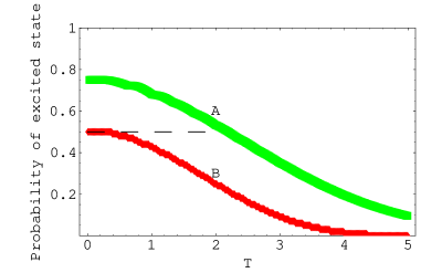
Figure 1: Probability distributions as functions of $T$ for two-state systems, illustrating the cases of (A) $|\langle g(0)|e(T)\rangle|^{2}=3/4>1/2$ and (B) $|\langle g(0)|e(T)\rangle|^{2}=1/2$. For the first case, there is a range of $T$ which violates (41), while in the latter we always have (41). The excited-state probability always approaches zero for sufficiently large $T$ according to the Quantum Adiabatic Theorem.

When the above is generalised to dimensionally infinite systems of the quantum algorithm for Hilbert’s tenth problem, the counterpart of (25) is the set of differential equations connecting the sets of instantaneous eigenstates of ${\cal H}(t)$ at different time $t$ Kieu (2003d). There, our choice of the coherent state (4), as the ground state in which the system initially has to be, entails that the condition (42) is always satisfied, since for any $n$ and $\alpha$

$$|\langle\alpha|n\rangle|^{2} = e^{-|\alpha|^{2}}\frac{|\alpha|^{2n}}{n!}<\frac{1}{2}.$$ (44)

And we expect that, in these infinite systems too, the probability to be subsequently found in any particular excited state cannot be greater than $\frac{1}{2}$ at anytime. Such arguments have also been numerically confirmed in several simulations of our algorithm Kieu (2003c, e) and also of a modified version Sicard et al. (2003).

V How can we compute the non-computable?

When proposed the tenth problem in 1900, Hilbert himself never anticipated the link it would have with what is the Turing halting problem of the yet-to-be-born field of Theoretical Computer Science. The Turing halting problem was only introduced and solved in 1937 by Turing, and the link of equivalence between the two problems was only established in 1972 Matiyasevich (1993).

V.1 The Turing halting problem

The question of the Turing halting problem can be phrased as whether there exists a universal process according to which it can be determined by a finite number of operations if any given Turing machine would eventually halt (in finite time) starting with some specific input. Turing raised this problem in parallel similarity to the Gödel’s Incompleteness Theorem and settled it with the result that there exists no such recursive universal procedure. The proof is based on Cantor’s diagonal arguments, also employed in the proof of the Incompleteness Theorem.

The proof is by contradiction starting with the assumption that there exists a recursive (and hence Turing computable) single-valued halting function $h(p,i)$ which accepts two integer inputs: $p$, the Gödel encoded integer for the Turing machine in consideration, and $i$, the Gödel encoded integer for the input for $p$,

$$h(p,i) = \left\{\begin{tabular}[]{l}0 \mbox{ if $p$ halts on input $i$};\\ 1 \mbox{ otherwise}.\end{tabular}\right.$$ (47)

One can then construct a program $Turing(n)$ having one integer argument $n$ in such a way that it calls the function $h(n,n)$ as a subroutine and then halts if and only if $h(n,n)=1$. In some made-up language:

(54)

Let $t$ be the Gödel encoded integer for $Turing$; we now apply the assumed halting function $h$ to $t$ and $n$, then clearly:

$$h(t,n)=0 \mbox{\bf if and only if }Turing\mbox{ halts on }n$$ (55)

$$\mbox{\bf if and only if }h(n,n)=1,$$

from which a contradiction is clearly manifest once we choose $n=t$.

The elegant proof above was only intended by Turing for the non-existence of a recursive halting function. Unfortunately, some has used this kind of arguments to argue that there cannot exist any halting function in general! We have pointed out elsewhere Ord and Kieu (2003b) the fallacies in such use, and considered carefully the implicit assumptions of Cantor’s diagonal arguments. See also the Subsection V.3 below.

V.2 The equivalence between Hilbert’s tenth and the Turing halting problem

It is easy to see that if one can solve the Turing halting problem one can then solve Hilbert’s tenth problem. This is accomplished by constructing a simple program that systematically searches for the zeros of a given Diophantine equation by going through the non-negative integers one by one and stops as soon as a solution is found. The Turing halting function (existed by assumption) can then be applied to that program to see if it ever halts or not. It halts if and only if the Diophantine equation has a non-negative integer solution.

Proving the relationship in the opposite direction, namely that if Hilbert’s tenth problem can be solved then will be Turing halting problem, is much harder and requires the so-called Davis-Putnam-Robinson-Matiyasevich (DPRM) Theorem Matiyasevich (1993):

Every recursively enumerable (r.e.) set  of n-tuple of non-negative integers has a Diophantine representation. That is, for every such r.e. set there is a unique family of Diophantine equations $D(a_{1},\ldots,a_{n};x_{1},\ldots,x_{m})=0$, each of which has $n$ non-negative integral parameters $(a_{1},\ldots,a_{n})$ and some $m$ variables $(x_{1},\ldots,x_{m})$, in such a way that a particular $n$-tuple $(a_{1},\ldots,a_{n})$ belongs to the set if and only if the Diophantine equation corresponding to the same $n$ parameters has some integer solutions .

Let us number all Turing machines (that is, programs in some fixed programming language) uniquely in some lexicographical order, say. The set of all non-negative integer numbers corresponding to all Turing machines that will halt when started from the blank tape is clearly a r.e. set. Let us call this set the halting set, and thanks to the DPRM Theorem above we know that corresponding to this set there is a family of one-parameter Diophantine equations. If Hilbert’s tenth problem were recursively soluble, that is, were there a recursive method to decide if any given Diophantine equation has any solution then we could have recursively decided if any Turing machine would halt when started from the blank tape. We just need to find the number representing that Turing machine and then decide if the relevant Diophantine equation having the parameter corresponding to this number has any solution or not. It has a solution if and only if the Turing machine halts.

But that would have contradicted the Cantor’s diagonal arguments for the Turing halting problem! Thus, one comes to the conclusion that there is no single recursive method for deciding Hilbert’s tenth problem. For the existence or lack of solutions of different Diophantine equations one may need different (recursive) methods anew each time.

Now, having reached this conclusion, we wish to point out that logically there is nothing wrong if there exist non-recursive or non-deterministic or probabilistic methods for deciding Hilbert’s tenth.

V.3 The quantum algorithm in context

In claiming that our quantum algorithm can somehow compute the noncomputable, we also need to consider it in the context of the no-go arguments above. Those arguments, indeed, cannot be applicable here because of several reasons. First of all, the proof for the working of our algorithm is not quite constructive, implying its non-recursiveness in some sense. The mathematical proof for the criterion for ground-state identification, as can be seen from the Section IV, is highly non-constructive as we have had to employ at several places the methods of proof by contradiction and also of (non-constructive) analysis for continuous functions.

Secondly, and more explicitly, our algorithm is outside the jurisdiction of those no-go arguments because of its probabilistic in nature. We have argued elsewhere Ord and Kieu (2003a) against the common misunderstanding that probabilistic computation is equivalent in terms of computability to Turing recursive computation. They are not! We have pointed out that if a non-recursively biased coin is used as an oracle for a computation, the computation carries more computability than Turing computation in general. Here, we shall show explicitly in the below how the probabilistic nature of our algorithm can avoid the Cantor’s diagonal no-go arguments presented in Subsection V.1 .

Because our algorithm is probabilistic (see Subsection II.2), we can only obtain an answer with certain probability to be the correct answer. This probability can be, with more and more work done, made arbitrarily closed, but never equal, to one as shown in (11). Thus, instead of the halting function (47) our algorithm can only yield a probabilistic halting function $ph$, similar but not quite the same as it must have three arguments instead of two,

$$ph(p,i,\delta) = \left\{\begin{tabular}[]{l}0 \mbox{ if $p$ halts on input $i$, with maximun error-probability $\delta$};\\ 1 \mbox{ if does not halt, with maximun error-probability $\delta$}.\end{tabular}\right.$$ (58)

In order to follow the Cantor’s arguments as closely as possible, we need to restrict to

$$\delta=2^{-J},$$ (59)

for some integer $J$. Following the flow of Cantor’s arguments, one can then construct a program $pTuring(n,\delta)$ having arguments $n$ and $\delta$ in such a way that it calls the function $ph(n,n,\delta)$ as a subroutine and then halts if and only if $ph(n,n,\delta)=1$. In some made-up language:

(66)

Similarly, let $t_{p}$ be the Gödel encoded integer for $pTuring$ (barring the case $pTuring$ does not have an integer encoding, which is quite possible for a quantum algorithm Kieu (2003b)). We next apply the probabilistic halting function $ph$ to $t_{p}$ and $(n,\delta)$, which is the total input for $pTuring$, and with some $\delta^{\prime}$, to obtain:

$$ph(t_{p},\tilde{n},\delta^{\prime})=0 \mbox{\bf iff }pTuring\mbox{ halts on $\tilde{n}$, with maximum error-probability $\delta^{\prime}$},$$ (67)

where $\tilde{n}$ encodes $(n,\delta)$ uniquely, that is, $\tilde{n}=p_{1}^{n}p_{2}^{J}$, where $p_{1}$ and $p_{2}$ are two different prime numbers. No matter what we choose for $n$ and $\delta^{\prime}$ and $J$, we cannot diagonalise the above, because $\tilde{n}\not=n$, unlike previously (55). Thus we never run into mathematical contradiction here.

The above arguments apparently have nothing to do with being quantum mechanical, but everything to do with being probabilistic. Quantum mechanics, however, has given us an inspiration to realise a probabilistic algorithm capable of deciding Hilbert’s tenth problem with a single, universal procedure for any input of Diophantine equations.

VI Concluding remarks

In this paper we have provided the analytical results and arguments for the working of our quantum algorithm for Hilbert’s tenth problem. Numerical simulations for some simple Diophantine equations have been preliminarily reported in Kieu (2003c) and will be available fully elsewhere Kieu (2003e), where we shall explain how to cope with the required dimensionally-unbounded Hilbert space and also argue that while the algorithm has been inspired by (quantum mechanical) physical processes it may be simulated on Turing computers, despite the proof that Hilbert’s tenth problem is recursively noncomputable.