Two and Three Qubits Geometry and Hopf Fibrations

Abstract.

This paper reviews recent attempts to describe the two- and three-qubit Hilbert space geometries with the help of Hopf fibrations. In both cases, it is shown that the associated Hopf map is strongly sensitive to states entanglement content. In the two-qubit case, a generalization of the one-qubit celebrated Bloch sphere representation is described.

1. Introduction

Two-level quantum systems, denoted qubits, have gained a renewed interest in the past ten years, owing to the fascinating perspectives of quantum information[1]. Having in mind the different qubit manipulation protocols that are proposed in this growing field, it is therefore of high interest to represent their quantum evolution in a suitable representation space, in order to get some insight into the subtleties of this complicated problem. For single two-level systems, a well known tool in quantum optics is the Bloch sphere representation, where the simple qubit state is faithfully represented, up to a global phase, by a point on a standard sphere $S^{2}$, whose coordinates are expectation values of physically interesting operators for the given quantum state. Guided by the relation between the Bloch sphere and a geometric object called the Hopf fibration of the $S^{3\text{ }}$hypersphere[4], a generalization for a two-qubit system was recently proposed[5], in the framework of the (high dimensional) $S^{7}$ sphere Hopf fibration, and will be recalled below. An interesting result is that the $S^{7}$ Hopf fibration is entanglement sensitive and therefore provides a kind of ”stratification”  for the 2 qubits states space with respect to their entanglement content. An extension of this description to a three qubits system, using the $S^{15}$ Hopf fibration, will also be presented here.

We first briefly remind known facts about the Bloch sphere representation, and its close relation to the $S^{3}$ Hopf fibration. We then recall in some details what was recently done for the two-qubit case in terms of the $S^{7}$ Hopf fibration. The $S^{15}$ Hopf fibration is then introduced, which helps describing the three-qubits Hilbert space geometry. As far as computation is concerned, going from the $S^{3}$ to the $S^{7}$ and then the $S^{15}$ fibrations merely amounts to replacing complex numbers by quaternions and then octonions. This is why a brief introduction to quaternions and octonions is given in appendix. Note that using these two kinds of generalized numbers is not strictly necessary here, but they provide an elegant way to put the calculations into a compact form, and have (by nature) a natural geometrical interpretation

2. From the S³ hypersphere to the Bloch sphere representation

A (single) qubit state reads

(1) $$\left|\Psi\right\rangle=\alpha\left|0\right\rangle+\beta\left|1\right\rangle,\qquad\alpha,\beta\in\mathbb{C}\mathbf{,\qquad}\left|\alpha\right|^{2}+\left|\beta\right|^{2}=1$$

In the spin ${\frac{1}{2}}$ context, the orthonormal basis $\left\{\left|0\right\rangle,\left|1\right\rangle\right\}$ are the two eigenvectors of the (say) $\sigma_{z}$ (Pauli spin) operator. Viewed as pairs of real numbers, the two normalized components $\alpha,\beta$ generate a unit radius sphere S³ embedded in R⁴. To take into account the global phase freedom, one expects to find a way to fill S³ with circles (the orbit of a global phase $\exp i\omega$ multiplying the pair ($\alpha,\beta$)), such that each state belongs to exactly one such circle. This task is nicely fulfilled by the so-called S³ Hopf fibration [2].

A fibred space $E$ is defined by a (many-to-one) map from $E$ to the so-called ”base space”, all points of a given fibre $F$ being mapped onto a single base point. A fibration is said ”trivial” if the base $B$ can be embedded in the fibred space $E$, the latter being faithfully described as the direct product of the base and the fibre (think for instance of fibrations of $R^{3}$ by parallel lines $R$ and base $R^{2}$ or by parallel planes $R^{2}$ and base $R$).

The simplest, and most famous, example of a non trivial fibration is the Hopf fibration of $S^{3}$ by great circles $S^{1}$ and base space $S^{2}$. For the qubit Hilbert space purpose, the fibre represents the global phase degree of freedom, and the base $S^{2}$ is identified to the Bloch sphere. One standard notation for a fibred space is that of a map $E\overset{F}{\rightarrow}B$, which reads here $S^{3}\overset{S^{1}}{\rightarrow}S^{2}$. Its non trivial character implies $S^{3}\neq S^{2}\times S^{1}$. This translates into the known failure in ascribing consistantly a definite phase to each representing point on the Bloch sphere.

To describe this fibration in an analytical form, we go back to the definition of $S^{3}$ as pairs of complex numbers $\left(\alpha,\beta\right)$ which satisfy $\left|\alpha\right|^{2}+\left|\beta\right|^{2}=1$. The Hopf map is defined as the composition of a map $h_{1}$ from $S^{3}$ to $R^{2}$ $(+\infty)$, followed by an inverse stereographic map $h_{2\text{ }}$from $R^{2}$ to $S^{2}:$

(4) $$h_{1} :\begin{array}[c]{ccc}S^{3}&\longrightarrow&R^{2}+\left\{\infty\right\}\\ \left(\alpha,\beta\right)&\longrightarrow&C=\overline{\alpha\beta^{-1}}\end{array}\qquad\alpha,\beta\in\mathbb{C}$$

(7) $$h_{2} :\begin{array}[c]{ccc}R^{2}+\left\{\infty\right\}&\longrightarrow&S^{2}\\ C&\longrightarrow&M(X,Y,Z)\end{array}\qquad X^{2}+Y^{2}+Z^{2}=1$$

where $\overline{z}$ is the complex conjugate of $z$). The first map $h_{1}$ clearly shows that the full $S^{3}$ great circle, parametrized by ($\alpha\exp i\omega,\beta\exp i\omega$), is mapped onto the same single point with complex coordinate $C$. It is easy to show that, with $R^{2}$ cutting the unit radius $S^{2}$ along the equator, and the north pole (along the $Z$ axis) as the stereographic projection pole, the $S^{2}$ Hopf fibration base coordinates coincide with the well known $S^{2}$ Bloch sphere coordinates :

(8) $$X =\left\langle\sigma_{x}\right\rangle_{\Psi}=2\operatorname{Re}(\overline{\alpha}\beta)$$

$$Y =\left\langle\sigma_{y}\right\rangle_{\Psi}=2\operatorname{Im}(\overline{\alpha}\beta)$$

$$Z =\left\langle\sigma_{z}\right\rangle_{\Psi}=\left|\alpha\right|^{2}-\left|\beta\right|^{2})$$

This correspondance between Hopf map and Bloch sphere is not new [4], but is poorly known in both communities (quantum optics and geometry). It is striking that the simplest non trivial object of quantum physics, the two-level system, bears such an intimate relation with the simplest non trivial fibred space.

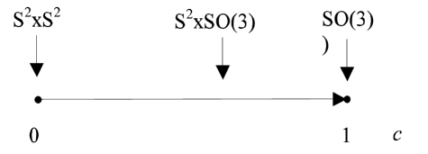
Figure 1. Foliation of the two-qubits Hilbert space with respect to state entanglement

It is tempting to try to visualize the full ($S^{3}$) Hilbert space with its fibre structure. This can be achieved by doing a (direct) stereographic map from $S^{3}$ to $R^{3}$ (figure 1). Each $S^{3}$ circular fibre is mapped onto a circle in $R^{3}$, with an exceptional straight line, image of the unique $S^{3}$ great circle passing through the projection pole.

Figure 1 : $S^{3}$ Hopf fibration after a stereographic map onto $R^{3}$. Circular $S^{1}$ fibres are mapped onto circles in $R^{3}$, except the exceptional fibre through the projection pole, which is mapped onto a vertical straight line. Fibres can be grouped into a continuous family of nested tori, three of which are shown here

3. Two qubits, entanglement and the $S^{7}$ Hopf fibration

3.1. The two-qubits Hilbert space

We now proceed one step further, and investigate pure states for two qubits. The Hilbert space $\mathcal{E}$ for the compound system is the tensor product of the individual Hilbert spaces $\mathcal{E}_{1}\otimes$ $\mathcal{E}_{2}$, with a direct product basis $\left\{\left|00\right\rangle,\left|01\right\rangle,\left|10\right\rangle,\left|11\right\rangle\right\}$. A two-qubit state reads

(9) $$\left|\Psi\right\rangle =\alpha\left|00\right\rangle+\beta\left|01\right\rangle+\gamma\left|10\right\rangle+\delta\left|11\right\rangle\qquad$$

$$\text{with \ }\alpha,\beta,\gamma,\delta \in\mathbb{C},\;\text{and }\left|\alpha\right|^{2}+\left|\beta\right|^{2}+\left|\gamma\right|^{2}+\left|\delta\right|^{2}=1$$

$\left|\Psi\right\rangle$ is said ”separable” if it can be written as a simple product of individual kets belonging to $\mathcal{E}_{1}$ and $\mathcal{E}_{2}$ separately, a definition which translates into the well known following condition : $\alpha\delta=\beta\gamma$. A generic state is not separable, and is said to be ”entangled”. The $\left|\Psi\right\rangle$ normalization condition $\left|\alpha\right|^{2}+\left|\beta\right|^{2}+\left|\gamma\right|^{2}+\left|\delta\right|^{2}=1$ identifies $\mathcal{E}$ to the 7-dimensional sphere $S^{7}$, embedded in $R^{8}$. It was therefore tempting to see whether the known $S^{7}$ Hopf fibration (with fibres $S^{3}$ and base $S^{4})$ can play any role in the Hilbert space description. This is the case indeed, as we have shown recently [5]. Let us summarize the main results, keeping in mind that some notations has been changed as compared to this latter reference.

3.2. The $S^{7}$ Hopf fibration

One follows the same line as in the $S^{3}$ case, but using quaternions instead of complex numbers (see appendix). We write

(10) $$q_{1}=\alpha+\beta\mathbf{j},\;q_{2}=\gamma+\delta\mathbf{j},\qquad q_{1,}q_{2}\in\mathbb{Q}\mathbf{,}$$

and a point (representing the state $\left|\Psi\right\rangle$) on the unit radius $S^{7}$ as a pair of quaternions $\left(q_{1,}q_{2}\right)$ satisfying $\left|q_{1}\right|^{2}+\left|q_{2}\right|^{2}=1$. The Hopf map from $S^{7}$ to the base $S^{4}$ is the composition of a map $h_{1}$ from $S^{7}$ to $R^{4}$ $(+\infty)$, followed by an inverse stereographic map $h_{2}$ from $R^{4}$ to $S^{4}$.

(13) $$h_{1} :\begin{array}[c]{ccc}S^{7}&\longrightarrow&R^{4}+\left\{\infty\right\}\\ \left(q_{1},q_{2}\right)&\longrightarrow&Q=\overline{q_{1}q_{2}^{-1}}\end{array}\qquad q_{1,}q_{2}\in\mathbb{Q}$$

(16) $$h_{2} :\begin{array}[c]{ccc}R^{4}+\left\{\infty\right\}&\longrightarrow&S^{4}\\ Q&\longrightarrow&M(x_{l})\end{array}\qquad\sum\limits_{l=0}^{l=4}x_{l}^{2}=1$$

The base space $S^{4}$ is not embedded  in $S^{7}$ : the fibration is again not trivial. The fibre is a unit $S^{3}$ sphere as can seen easily by remarking that the $S^{7}$ points $\left(q_{1,}q_{2}\right)$ and $\left(q_{1}q,\,q_{2}q\right)$, with $q$ a unit quaternion (geometrically a $S^{3}$ sphere) are mapped onto the same $Q$ value.

The $h_{1}$ map leads to

(17) $$Q =\overline{q_{1}q_{2}^{-1}}=\frac{1}{\sin^{2}\left(\theta/2\right)}\left[\overline{\left(\alpha+\beta\mathbf{j}\right)\left(\overline{\gamma}-\delta\mathbf{j}\right)}\right]=\frac{1}{\sin^{2}\left(\theta/2\right)}\left(C_{1}+C_{2}\mathbf{j}\right)$$

$$\text{with }\sin\left(\theta/2\right) =\left|q_{2}\right|\text{, }C_{1}=\left(\overline{\alpha}\gamma+\overline{\beta}\delta\right),\text{ }C_{2}=\left(\alpha\delta-\beta\gamma\right)\text{ and }C_{1},C_{2}\in\mathbb{C}$$

We face here a first striking result: the Hopf map is entanglement sensitive! Indeed, non entangled states satisfy $\alpha\delta=\beta\gamma$ and therefore map onto the subset of pure complex numbers in the quaternion field (both being completed by $\infty$ when the $Q$ denominator vanishes3). Geometrically, this means that non-entangled states map from $S^{7}$ onto a 2-dimensional planar subspace of the target space $R^{4}$.

The second map $h_{2\text{ }}$sends states onto points on $S^{4}$, with coordinates $x_{l}$, with $l$ running from to $0$ to $4$. With the inverse stereographic pole located on the $S^{4}$ ”north pole ” ($x_{0}=+1$), and the target space $R^{4\text{ }}$ cutting $S^{4}$ along the equator, we get the following coordinate expressions

(18) $$x_{0} =\cos\theta=\left|q_{1}\right|^{2}-\left|q_{2}\right|^{2}$$

$$x_{1} =\sin\theta\;S(Q^{\prime})=2\operatorname{Re}\left(\overline{\alpha}\gamma+\overline{\beta}\delta\right)$$

$$x_{2} =\sin\theta\;V_{\mathbf{i}}(Q^{\prime})=2\operatorname{Im}\left(\overline{\alpha}\gamma+\overline{\beta}\delta\right)$$

$$x_{3} =\sin\theta\;V_{\mathbf{j}}(Q^{\prime})=2\operatorname{Re}\left(\alpha\delta-\beta\gamma\right)$$

$$x_{4} =\sin\theta\;V_{\mathbf{k}}(Q^{\prime})=2\operatorname{Im}\left(\alpha\delta-\beta\gamma\right)$$

$Q^{\prime}$ is the normalized image of the $h_{1}$ map ($Q^{\prime}=\tan\left(\theta/2\right)Q$), $S(Q^{\prime})$ and $V_{\mathbf{i},\mathbf{j},\mathbf{k}}(Q^{\prime})$ being respectively the scalar and vectorial parts of the quaternion $Q^{\prime}$ (see appendix). As for the standard Bloch sphere case, the $x_{l}$ coordinates are also expectation values of simple operators in the two-qubits state. An obvious one is $x_{0}$ which corresponds to $\left\langle\sigma_{z}\otimes Id\right\rangle_{\Psi}$. The two next coordinates are also easily recovered as

(19) $$x_{1} =2\operatorname{Re}\left(\overline{\alpha}\gamma+\overline{\beta}\delta\right)=\left\langle\sigma_{x}\otimes Id\right\rangle_{\Psi}$$

$$x_{2} =2\operatorname{Im}\left(\overline{\alpha}\gamma+\overline{\beta}\delta\right)=\left\langle\sigma_{y}\otimes Id\right\rangle_{\Psi}$$

The remaining two coordinates, $x_{3}$ and $x_{4}$, are also expectation values of an operator acting on $\mathcal{E}$, but in a more subtle way. Define $\mathbf{J}$ as the (antilinear) ”conjugator”, an operator which takes the complex conjugate of all complex numbers involved in an expression (here acting on the left in the scalar product below). Form then the antilinear operator $\mathbf{E}$ (for ”entanglor”): $\mathbf{E}=-\mathbf{J}\left(\sigma_{y}\otimes\sigma_{y}\right)$. One finds

$$x_{3} =\operatorname{Re}\left\langle\mathbf{E}\right\rangle_{\Psi}$$

$$x_{4} =\operatorname{Im}\left\langle\mathbf{E}\right\rangle_{\Psi}.$$

Note that $\left\langle\mathbf{E}\right\rangle_{\Psi}$ vanishes for non entangled states, and takes its maximal norm (equals to 1) for maximally entangled states.  Such an operator, which is nothing but the time reversal operator for two spins ${\frac{1}{2}}$, is already widely used in quantifying entanglement[7], through a quantity called the ”concurrence” $c$, which corresponds here to $c=2\left|C_{2}\right|$.

3.3. Generalized Bloch sphere for the two-qubit case

Let us first inverse the Hopf map, and get the general expression for the set of states ( a $S^{3}$ sphere in $S^{7}$) which is sent to $Q$ by the $h_{1}$ map. A generic such state, noted $\Psi_{Q}$, reads (given as a pair of quaternions)

(20) $$\Psi_{Q}=(\cos\left(\theta/2\right)\,q\,,\sin\left(\theta/2\right)Q^{\prime}\,q),$$

with $q$ a unit quaternion spanning the $S^{3}$ fibre. Notice that we could also write $\Psi_{Q}$ in a way that recall the standard spinor notation (but here with quaternionic instead of complex components):

(21) $$\Psi_{Q}=(\cos\left(\theta/2\right)\exp\left(-\varphi\mathbf{t}/2\right)\,q\,,\sin\left(\theta/2\right)\exp\left(\varphi\mathbf{t}/2\right)\,q),$$

where $\cos\varphi=x_{1}/\sin\theta=S(Q^{\prime})$, and $\mathbf{t}$ is the following unit pure imaginary quaternion :

(22) $$\mathbf{t=}\left(\mathbf{V}_{\mathbf{i}}(Q^{\prime})\mathbf{i}+\mathbf{V}_{\mathbf{j}}(Q^{\prime})\mathbf{j}+\mathbf{V}_{\mathbf{k}}(Q^{\prime})\mathbf{k}\right)/\sin\varphi.$$

In order to compare with the generic expression (9), we aim to write $\Psi_{Q}$ as a quadruplet of complex numbers. For that purpose, we express the two unit quaternions $q$ and $Q^{\prime}$ in terms of pairs of complex numbers, $q=a+b\mathbf{j}$ (with $\left|a\right|^{2}+\left|b\right|^{2}=1$), and $Q^{\prime}=u+v\mathbf{j}$ (with $\left|u\right|^{2}+\left|v\right|^{2}=1$), and eventually get:

(23) $$\Psi_{Q}=(\cos\left(\theta/2\right)a\,,\cos\left(\theta/2\right)b,\sin\left(\theta/2\right)(ua-v\overline{b}),\sin\left(\theta/2\right)(ub+v\overline{a}))$$

In the above expression, $\theta,$ $u$ and $v$ correspond to the base space part of the fibration. Furthermore, we can relate $u$ and $v$ to already known quantities. Indeed

$$u=(x_{1}+\mathbf{i}x_{2})/\sin\theta=\left\langle\left(\sigma_{x}+\mathbf{i}\sigma_{y}\right)\otimes Id\right\rangle_{\Psi}/\sin\theta.$$

In addition, the state global phase indeterminacy allows to take $v$ a real. More precisely

$$v=c/\sin\theta\text{\ , where }c\text{ is the above mentionned concurrence}$$

Let us now describe the two extreme cases of separable and maximally entangled states.

3.3.1. Separable states

In the non entangled case, we have seen above that $Q$ is a complex number, $\mathbf{t}=\mathbf{i,}$ and therefore $u=\exp\mathbf{i}\varphi$ and $v=0$. The above expression simplifies to

(24) $$\Psi_{Q}=(\cos\left(\theta/2\right)\,a,\cos\left(\theta/2\right)b,\sin\left(\theta/2\right)\,a\exp\mathbf{i}\varphi,\sin\left(\theta/2\right)b\exp\mathbf{i}\varphi).$$

Up to a global rescaling by $\exp\left(-\mathbf{i}\varphi/2\right)$, one gets the following ket $\left|\Psi_{Q}\right\rangle$:

(25) $$\left|\Psi_{Q}\right\rangle=\left(\cos\left(\theta/2\right)\exp\left(-\mathbf{i}\varphi/2\right)\left|0\right\rangle_{1}+\sin\left(\theta/2\right)\exp\left(\mathbf{i}\varphi/2\right)\left|1\right\rangle_{1}\right)\otimes\left(\,a\left|0\right\rangle_{2}+b\left|1\right\rangle_{2}\right)$$

The projective Hilbert space for two non-entangled qubits is known to be the product of two 2-dimensional spheres $S_{1}^{2}\times S_{2}^{2}$, each sphere being the Bloch sphere associated with the given qubit. This property is clearly displayed here. The unit $S^{4}$ base space reduces to a unit $S^{2}$ sphere (since $x_{3}=x_{4}=0)$ which is nothing but the Bloch sphere for the first qubit. The second qubit Bloch sphere is then recovered from the fibre, spanned by $q=a+b\mathbf{j}$.  Indeed, we can iterate the fibration process on the $S^{3}$ fibre itself and get the (Hopf fibration base)-(Bloch sphere) coordinates for this two-level system. It is now easy to recover that this new $S^{2}$ base is the second qubit Bloch sphere.

In summary, for non entangled qubits, the $S^{7}$ Hopf fibration, with base $S^{4}$ and fibre $S^{3}$, simplifies to the simple product of a $S^{2}$ sub-sphere of the base (the first qubit Bloch sphere) by a second $S^{2}$ (the second qubit Bloch sphere) obtained as the base of a $S^{3}$ Hopf fibration applied to the fibre itself. Let us stress that this last iterated fibration is necessary to take into account the global phase of the two qubit system.

The fact that these two $S^{2}$ spheres play a symmetrical role (although one is related to the base and the other to the fibre) can be understood in the following way. We grouped together $\alpha$ and $\beta$ on one hand, and $\gamma$ and $\delta$ on the other hand, to form the quaternions $q_{1}$ and $q_{2}$, and then define the Hopf map $h_{1}$ as the ratio of these two quaternions (plus a complex conjugation). Had we grouped $\alpha$ and $\gamma$, and $\beta$ and $\delta$, to form two new quaternions, and use the same definition for the Hopf map, we would also get a $S^{7}$ Hopf fibration, but differently oriented. We let as an exercise to compute the base and fibre coordinates in that case. The net effect is to interchange the role of the two qubits: the second qubit Bloch sphere is now part of the $S^{4}$ base, while the first qubit Bloch sphere is obtained from the $S^{3}$ fibre.

3.3.2. Maximally entangled states

Let us now focus on maximally entangled states (M.E.S.). They correspond to the complex number $C_{2}$ having maximal norm $1/2$ (unit concurrence). This in turn implies that the Hopf map base reduces to a unit circle in the plane $\left(x_{3},x_{4}\right)$, parametrized by the unit complex number $2C_{2}$. The projective Hilbert space for these M.E.S. is known to be $S^{3}/Z_{2},$ a $S^{3}$  sphere with identified opposite points [3] (this is linked to the fact that all M.E.S. can be related by a local operation on one sub-system, since $S^{3}/Z_{2}=SO(3)$). In order to recover this result in the present framework, one can follow the trajectory of a representative point on the base and on the fibre while the state is multiplied by an overall phase $\exp\left(i\omega\right)$. The expression for $C_{2}\left(=\alpha\delta-\beta\gamma\right)$ shows that the point on the base turns by twice the angle $\omega$. Only when $\omega=\pi$ does the corresponding state belongs to the same fiber (e.g. maps onto the same value on the base). The fact that the fibre is a $S^{3}$ sphere, and this two-to-one correspondance between the fibre and the base under a global phase change, explains the $S^{3}/Z_{2}$ topology for the M.E.S. projective Hilbert space. Let us give now a more explicit proof of that result.

M.E.S.correspond to $\theta=\pi/2$ and maximal concurrence ($c=1$), which leads to $u=0$ and $v=1$. $\Psi_{MES}$ therefore read , from expression (23):

(26) $$\Psi_{MES}=\frac{1}{\sqrt{2}}(a,b\,,-\overline{b},\overline{a}).$$

The latter expression (26) for maximally entangled states is rather interesting in that it directly shows the $S^{3}/Z_{2}$ topology for the M.E.S. projective Hilbert space. Indeed, the M.E.S. set corresponds to pairs $\left(a,b\right)$, which as a whole cover a unit radius $S^{3}$ sphere. Now, looking to the quadruplet expression ($\ref{Psi_MES1}),$ opposite points $(a,b)$ and $(-a,-b)$ on $S^{3}$ clearly correspond to the same state $\Psi_{MES}$ (up to a global phase). Opposite points on $S^{3}$ have therefore tobe identified, leading to the $S^{3}/Z_{2}$ ($\equiv SO(3)$) structure.

This one-to-one correspondance between M.E.S. and 3 dimensional rotation matrices has recently led to propose using the former in an ”applied topology” experiment [8]: to verify experimentally the well known subtle topology of the (two-fold connected) $SO(3)$ group. The latter property is evidenced by constructing the two inequivalent family of closed paths in the geometrical manifold representing this group. This is done by choosing sequences of unitary operations on the MES two-qubits states. The non equivalence between the two paths is manifested by a $\pi$ topological phase shift which should result from an adequate interference experiment (a twin photons experiment have been proposed, but other two-qubit states could be used).

3.3.3. A generalization of the Bloch sphere representation

We are now led to consider a generalization of the Bloch sphere for the two-qubit projective Hilbert space. Clearly, the present Hopf fibration description suggests a splitting of the representation space in a product of base and fibres sub-spaces. Of the base space $S^{4}$, we propose to only keep the first three coordinates

(27) $$\left(x_{0},x_{1},x_{2}\right)=\left(\left\langle\sigma_{z}\otimes Id\right\rangle_{\Psi},\left\langle\sigma_{x}\otimes Id\right\rangle_{\Psi},\left\langle\sigma_{y}\otimes Id\right\rangle_{\Psi}\right)$$

All states map inside a standard ball $B^{3}$ of radius 1, where the set of separable states forms the $S^{2}$ boundary (the usual first qubit Bloch sphere), and the centre corresponds to maximally entangled states. Concentric spherical shells around the centre correspond to states of equal concurrence $c$ (maximal at the centre, zero on the surface), the radius of the spherical shell being equal to $\sqrt{1-c^{2}}$. The idea of slicing the 2-qubit Hilbert space into manifolds of equal concurrence is not new [3],[9]. What is nice here is that, under the Hopf map (and a projection onto the 3d subspace of the base spanned by the first three coordinates), these manifolds transforms into concentric $S^{2}$ shells which fill the unit ball.

To each point ($x_{0},x_{1},x_{2}$), it corresponds a $S^{3}/Z_{2}$ manifold, spanned by the couple ($a,b$), as seen clearly from relation (23), with an added identification of ($a,b$) and ($-a,-b$). The natural generalization of the Bloch sphere for two qubits is therefore a product of two $B^{3}$ balls. The first one, spanned by the triple ($x_{0},x_{1},x_{2}$), has just been described as containing the partial Bloch sphere for one the two qubits, with its set of concentric iso-concurrence spheres. The second one corresponds to the standard representation of $SO(3)$ by a $\overleftrightarrow{B^{3}}$ ball of radius $\pi$, the double arrow sign recalling that opposite points on the boundary $S^{2}$ sphere have to be identified. This picture is valid for all states except the separable ones, for which the fiber derived $\overleftrightarrow{B^{3}}$ space reduces to a $S^{2}$ sphere (the second qubit partial Bloch sphere).

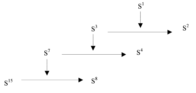
Figure 2. Figure 3: Nesting of the three Hopf fibrations

Instead of mapping the continuous set of $S^{2}$ spheres onto the filled ball $B^{3}$ in the space spanned by ($x_{0},x_{1},x_{2}$), this nice(but singular) foliation of the two-qubit projective Hilbert space (here the complex projective space $CP^{3})$ can be also pictured as a concurrence segment (between 0 and 1) with the corresponding sub-manifolds. The sub-space of vanishing concurrence has a $S^{2}\times S^{2}$ structure, while that of maximal ($c=1$) concurrence corresponds to $SO(3)$. Sub-manifolds of intermediate concurrence have the structure of a direct product $S^{2}\times SO(3)$, the sphere $S^{2}$ having radius $\sqrt{1-c^{2}}$. This illustrated in the figure 2 below

Examples

Back to to the $B^{3}$ picture, let us for instance go through the states along a simple $B^{3}$ ray, from the point $\left(0,1,0\right),$ image of the states $\Psi_{S}$ such that $\left\langle\sigma_{x}\otimes Id\right\rangle_{\Psi}=1$, to the $B^{3}$ center $\left(0,0,0\right)$, image the maximally entangled states $\Psi_{MES}$ . $Q^{\prime}$ reduces to a unit circle in the plane spanned by ($x_{1},x_{3}$), and these states are therefore parametrized by a single angle $\epsilon$ in the interval $\left[0,\pi/2\right]$,

(28) $$\Psi_{\epsilon}=\frac{1}{\sqrt{2}}(\,q\,,\exp\left(\epsilon\mathbf{j}\right)\,\,q).\text{,}$$

or, written as a quadruplet of complex numbers,

(29) $$\Psi_{\epsilon}=\frac{1}{\sqrt{2}}(a\,,b,a\cos\epsilon-\overline{b}\sin\epsilon,b\cos\epsilon+\overline{a}\sin\epsilon).$$

For $\epsilon=0$, one gets

(30) $$\Psi_{\epsilon=0} =\Psi_{S}=\frac{1}{\sqrt{2}}\left(a,b,a,b\right).\text{ and therefore}$$

$$\left|\Psi_{S}\right\rangle =\frac{1}{\sqrt{2}}\left(\left|0\right\rangle_{1}+\left|1\right\rangle_{1}\right)\otimes\left(a\left|0\right\rangle_{2}+b\left|1\right\rangle_{2}\right),$$

as expected for the set of separable states which are eigenstates of $\sigma_{x}\otimes Id$ (with eigenvalue $+1$).

For $\epsilon=\pi/2$, the above set of maximally entangled states, as given by relation (26), is recovered. Intermediate values of $\epsilon$ correspond to less entangled states, whose concurrence read $c=\sin\epsilon$, as can be easily found from equation (29). Expression (29) also proves that the set of such states describes a $S^{3}/Z_{2}$ manifold.

Similar analyses can be done for any path inside the $B^{3}$ ball. A second very simple example is provided by the path from $\left(1,0,0\right)$ to $\left(0,0,0\right)$. In that case the states, again parametrized by an angle $\epsilon$, read

$$\Psi_{\epsilon}=(\cos\frac{\epsilon}{2}a\,,\cos\frac{\epsilon}{2}b,-\sin\frac{\epsilon}{2}\overline{b},\sin\frac{\epsilon}{2}\overline{a}).$$

3.3.4. Relation with the Bloch ball representation for mixed states

The Bloch ball single qubit mixed state representation was recalled above. In that case, the centre of the Bloch ball corresponds to maximally mixed states. The reader should not be surprised to find here (in the two-qubits case) a second unit radius ball, with maximally entangled states now at the centre. It corresponds to a known relation between partially traced two-qubit pure states and one-qubit mixed state. Indeed the partially traced density matrix $\rho_{1}$ is simply written in terms of $C_{1}$ and $C_{2}$ derived from the $S^{7}$ Hopf map:

(31) $$\rho_{1}=\frac{1}{2}\left(\begin{array}[c]{cc}1+x_{0}&x_{1}-\mathbf{i\,}x_{2}\\ x_{1}+\mathbf{i\,}x_{2}&1-x_{0}\end{array}\right)=\left(\begin{array}[c]{cc}\left|q_{1}\right|^{2}&\overline{C_{1}}\\ C_{1}&\left|q_{2}\right|^{2}\end{array}\right)\text{ \ }$$

with unit trace and $\det\rho_{1}=\left|C_{2}\right|^{2}.$ The partial $\rho_{1}$ represents a pure state density matrix whenever $C_{2}$ vanishes (the separable case), and allows for a unit Bloch sphere (that associated to the first qubit). It corresponds to a mixed state density matrix as soon as $\left|C_{2}\right|>0$ (and an entangled state for the two qubit state). The other partially traced density matrix $\rho_{2}$ is related to the other $S^{7}$ Hopf fibration which was discussed above.

4. Three qubits, and the $S^{15}$ Hopf fibration

4.1. Three qubits

The Hilbert space $\mathcal{E}$ for the compound system is the tensor product of the individual Hilbert spaces $\mathcal{E}_{1}\otimes$ $\mathcal{E}_{2}\otimes$ $\mathcal{E}_{3}$, with a direct product basis

$$\left\{\left|000\right\rangle,\left|001\right\rangle,\left|010\right\rangle,\left|011\right\rangle,\left|100\right\rangle,\left|101\right\rangle,\left|110\right\rangle,\left|111\right\rangle\right\},$$

which can be written $\left\{\left|l\right\rangle,l=0..7\right\}$. A three-qubit state reads

$$\left|\Psi\right\rangle=\sum_{l=0}^{7}t_{l}\left|l\right\rangle\text{\ \ \ with \ }t_{l}\in\mathbb{C},\;\text{and }\sum\text{ }\left|t_{l}\right|^{2}=1$$

The $\left|\Psi\right\rangle$ normalization condition identifies $\mathcal{E}$ to the 15-dimensional sphere $S^{15}$, embedded in $R^{16}$. This suggests looking to how far the third Hopf fibration (that of $S^{15}$, with base $S^{8}$ and fibres $S^{7})$ can be helpful for describing the 3 qubits Hilbert space geometry.

4.2. The $S^{15}$ Hopf fibration

One proceeds along the same line as for the previous $S^{3}$ and $S^{7}$ cases, but using now octonions (see appendix). We write

(32) $$a=a^{\prime}+a"\mathbf{e},\;b=b^{\prime}+b"\mathbf{e},\qquad a,b\in\mathbb{O}_{,}\text{ and }a^{\prime},a",b^{\prime},b"\in\mathbb{Q}\mathbf{,}$$

and a point (representing the state $\left|\Psi\right\rangle$) on the unit radius $S^{15}$ as a pair of octonions $\left(a,b\right)$ satisfying $\left|a\right|^{2}+\left|b\right|^{2}=1$. But, to get a Hopf map of physical interest, with coordinates simply related to interesting observable expectation values, one needs to define a slightly tricky relation between $\left|\Psi\right\rangle$ and the octonions pair $\left(a,b\right)$, as follows:

(33) $$a =(t_{0}+t_{1}\mathbf{j,}t_{2}+\mathbf{j}t_{3})=(t_{0}+t_{1}\mathbf{j,}t_{2}+\overline{t_{3}}\mathbf{j})=\left(a^{\prime},a^{\prime\prime}\right)$$

$$b =(t_{4}+t_{5}\mathbf{j,}t_{6}+\mathbf{j}t_{7})=(t_{4}+t_{5}\mathbf{j,}t_{6}+\overline{t_{7}}\mathbf{j})=\left(b^{\prime},b^{\prime\prime}\right)$$

The Hopf map from $S^{15}$ to the base $S^{8}$ is the composition of a map $h_{1}$ from $S^{15}$ to $R^{8}$ $(+\infty)$, followed by an inverse stereographic map $h_{2}$ from $R^{8}$ to $S^{8}$.

(36) $$h_{1} :\begin{array}[c]{ccc}S^{15}&\longrightarrow&R^{8}+\left\{\infty\right\}\\ \left(a,b\right)&\longrightarrow&P=\overline{ab^{-1}}\end{array}\qquad a,b\in\mathbb{O}$$

(39) $$h_{2} :\begin{array}[c]{ccc}R^{8}+\left\{\infty\right\}&\longrightarrow&S^{8}\\ P&\longrightarrow&M(x_{l})\end{array}\qquad\sum\limits_{l=0}^{l=8}x_{l}^{2}=1$$

The base space $S^{8}$ is not embedded  in $S^{15}$ : the fibration is again not trivial.

The fibre is a unit $S^{7}$ sphere, the proof of which is more tricky (and not given here) than in the lower dimension case. The $h_{1}$ map leads to

(40) $$P =\overline{ab^{-1}}=\frac{1}{\sin^{2}\theta/2}\left(Q_{1}+Q_{2}\mathbf{e}\right)$$

$$\text{with }\sin\theta/2 =\left|b\right|\text{, }Q_{1}=(b^{\prime}\overline{a^{\prime}}+\overline{a^{\prime\prime}}b^{\prime\prime}),\text{ }Q_{2}=\left(-a^{\prime\prime}b^{\prime}+b^{\prime\prime}a^{\prime}\right)\text{ and }Q_{1},Q_{2}\in\mathbb{Q}$$

Athough this is not at first sight evident, the Hopf map is still entanglement sensitive in that case. To show this, it is instructive to first express $Q_{1}$ and $Q_{2}$ in term of the $t_{l}$ components read out from ($\ref{3qubit_octo}).$

$$Q_{1} =\left(\overline{t_{0}}t_{4}+\overline{t_{1}}t_{5}+\overline{t_{2}}t_{6}+\overline{t_{3}}t_{7})+(t_{0}t_{5}-t_{1}t_{4}+\overline{t_{2}}\overline{t_{7}}-\overline{t_{3}}\overline{t_{6}}\right)\,\mathbf{j}$$

$$Q_{2} =\left(t_{0}t_{6}+t_{2}t_{4}+\overline{t_{3}}\overline{t_{5}}-\overline{t_{1}}\overline{t_{7}})+(t_{1}t_{6}-t_{2}t_{5}+\overline{t_{0}}\overline{t_{7}}-\overline{t_{3}}\overline{t_{4}}\right)\,\mathbf{j}$$

Let us introduce the generalised complex concurrence terms $T_{ij,kl}=t_{i}t_{j}-t_{k}t_{l}$. They allow to write in a synthetic form the coordinates on the base $S^{8}.$ The second map $h_{2\text{ }}$sends states onto points on $S^{8}$, with coordinates $x_{l}$, with $l$ running from to $0$ to $8$. With the inverse stereographic pole located on the $S^{8}$ ”north pole ” ($x_{0}=+1$), and the target space $R^{8\text{ }}$ cutting $S^{8}$ along the equator, we get the following coordinate expressions

(41) $$x_{0} =\cos\theta=\left|a\right|^{2}-\left|b\right|^{2}=\left\langle\sigma_{z}\otimes Id\otimes Id\right\rangle_{\Psi}$$

$$x_{1}+\mathbf{i\,}x_{2} =2\left(\overline{t_{0}}t_{4}+\overline{t_{1}}t_{5}+\overline{t_{2}}t_{6}+\overline{t_{3}}t_{7}\right)=\left\langle\left(\sigma_{x}+\mathbf{i\,}\sigma_{y}\right)_{1}\otimes Id\otimes Id\right\rangle_{\Psi}$$

$$x_{3}+\mathbf{i\,}x_{4} =2\left(T_{05,14}+\overline{T_{27,36}}\right)$$

$$x_{5}+\mathbf{i\,}x_{6} =2\left(T_{06,24}+\overline{T_{35,17}}\right)$$

(42) $$x_{7}+\mathbf{i\,}x_{8} =2\left(T_{16,25}+\overline{T_{07,34}}\right)$$

A lengthy, but trivial, computation allows to verify that  the base $S^{8}$ has unit radius.

4.3. Discussion

It is easy to show that three-qubits states such that the first qubit is separated from the two others map onto a point such that $x_{j}=0,$ for $j=4,5,6,7,8.$ One way to show this is to realize that, in a multi-qubit state, a given qubit is separated from the others when its partial Bloch sphere has a unit radius. The first qubit partial Bloch sphere is spanned here by the triplet $(x_{0},x_{1},\mathbf{\,}x_{2}).$ A second proof consists in writing down the separability algebraic conditions [10]. In the present case, the latter imply that the above generalized concurrences vanish (in fact the six vanishing conditions only rely onto three independant conditions). Going back to the above definition of the $h_{1}$ map, this means that in that case, the Hopf map carries an octonion couple onto a pure complex number $P$. Therefore, as for two-qubits and $S^{7}$, the $S^{15\text{ }}$Hopf fibration is also entanglement sensitive for three qubits! This result has been independantly derived by Bernevig and Chen[11].

However, one should notice an important difference between the two- and three-qubit cases. In the two-qubit case, the $S^{7}$ Hopf fibration have allowed us to foliate the projective Hilbert space with respect to state entanglement, the latter, measured by the concurrence, being simply related to the norm the restriction of the base point to the subspace spanned by the triplet $(x_{3},x_{4}).$ Since the base space $S^{4}$ has unit radius, the entanglement is therefore simply related to the radius the first qubit partial Bloch sphere, spanned by the triplet $(x_{0},x_{1},\mathbf{\,}x_{2})$. The first-to-second qubit distinction (base-fibre in the fibration) do not matter here (to define the foliation) since the two partial Bloch sphere radii are equal.

The $S^{15\text{ }}$Hopf fibration is clearly sensitive to the entanglement of one qubit (the first qubit in the present case) with respect to the other two qubits: the first qubit partial Bloch sphere radius is still read out from the norm of the restriction of the base point to the subspace spanned by the triplet $(x_{0},x_{1},\mathbf{\,}x_{2})$. However, the latter does not tell the whole story in terms of state entanglement. Once you know how far qubit 1 is entangled with the remaining two, you do not yet know whether the second (or third) qubit is or not separated. This prevents from building a foliation driven by a single entanglement parameter. One possibility for such a foliation unique parameter would be to use the 3-tangle[12]. But it does not distinguish among separable and entangled W states. An alternative entanglement parameter has been by suggested by Bernevig and Chen [11] (see also ref.[13] for a related measure): to recover the symmetry between the three qubits, an average over the three qubits partial Bloch sphere radii is used.

The solution to the foliation problem might be to use three (instead of one) parameters, by considering three distinct $S^{15\text{ }}$Hopf fibrations, such that each of the three qubits partial Bloch spheres is singled out by the first three coordinates on the base. Said more simply, one may try to describe the Hilbert space geometry in a space spanned by the three partial Bloch sphere radii ($r_{1},r_{2},r_{3}$). Since each radius belongs to the interval $\left[0,1\right],$ the whole representation lies inside a unit cube. When one radius equals 1, one qubit is separated from the other two, and the other two radii are equal. We then see that the set under consideration cuts three square faces of the cube (such that $r_{j}=1),$ along a diagonal. These diagonals corresponds to the product of a sphere $S^{2}$ (the Bloch sphere of the separated qubit), and a copy of the above foliation for the remaining two qubits. Notice that the latter foliation was introduced above with respect to state entanglement, as measured by the concurrence $c$, instead of the partial Bloch sphere radius. To get a fully equivalent picture, one should therefore transform the original coordinate system from $c$ to $r=\sqrt{1-c^{2}}$.

5. Conclusion

Our main goal in this paper was to provide a geometrical representation of the two and three-qubit Hilbert space pure states. We have shown that, as for the one-qubit Bloch sphere relation to the $S^{3}$ Hopf fibration, the more complex $S^{7}$ and $S^{15}$ Hopf fibrations also play a natural role in that case. Note that, as already mentionned in ref. [5], in the three Hopf fibration sequence ($S^{15},S^{7},S^{3})$, the fibre in the larger dimensional space is the full space in next case. This is illustrated below:

This offers the possibility of further nesting the fibrations, a possibility that was already used in the present analysis of two-qubit separable case. This also applies to the three qubit case: whenever the first qubit is separated from the other two, the base reduces to the first qubit Bloch sphere, and the $S^{7}$ fibre is precisely the Hilbert space of the remaining two qubits.

In the two-qubit case, this approach has in particular allowed for a complete description of the pure state projective Hilbert space, in terms of an entanglement driven foliation, with well characterized leaves. This goal has not yet been achieved in the three qubits case, although a plausible track has been proposed here.

Appendix A Quaternions and Octonions

Quaternions

Quaternions are usually presented with the imaginary units $\mathbf{i},\mathbf{j}$ et $\mathbf{k}$ in the form :

$$q=x_{0}+x_{1}\mathbf{i}+x_{2}\mathbf{j}+x_{3}\mathbf{k},\qquad x_{0},x_{1},x_{2},x_{3}\in\mathbb{R}\quad\text{with }\mathbf{i}^{2}=\mathbf{j}^{2}=\mathbf{k}^{2}=\mathbf{ijk}=-1,$$

the latter ”Hamilton” relations defining the quaternion multiplication rules which are non-commutative. They can also be defined equivalently, using the complex numbers $c_{1}=x_{0}+x_{1}\mathbf{i}$ and $c_{2}=x_{2}+x_{3}\mathbf{i}$, in the form $q=c_{1}+c_{2}\mathbf{j}$, or equivalently as an ordered pair of complex numbers staisfying

$$\left(c_{1},c_{2}\right)+\left(d_{1},d_{2}\right) =\left(c_{1}+d_{1},c_{2}+d_{2}\right)$$

$$\left(c_{1},c_{2}\right)\left(d_{1},d_{2}\right) =\left(c_{1}d_{1}-c_{2}\overline{d_{2}},c_{1}d_{2}+c_{2}\overline{d_{1}}\right)$$

The conjugate of a quaternion $q$ is $\overline{q}=x_{0}-x_{1}\mathbf{i}-x_{2}\mathbf{j}-x_{3}\mathbf{k=}\overline{c_{1}}-c_{2}\mathbf{j}$ and its squared norm reads $N_{q}^{2}=q\overline{q}$.

Another way in which $q$ can be written is as a scalar part $S(q)$ and a vectorial part $\mathbf{V}(q)$:

$$q=S(q)+\mathbf{V}(q),\;S(q)=x_{0},\;\mathbf{V}(q)=x_{1}\mathbf{i}+x_{2}\mathbf{j}+x_{3}\mathbf{k,}$$

with the relations

$$S(q)=\frac{1}{2}(q+\overline{q}),\;\mathbf{V}(q)=\frac{1}{2}(q-\overline{q}).$$

A quaternion is said to be real if $\mathbf{V}(q)=0$, and pure imaginary if $S(q)=0$. We shall also write$\;\mathbf{V}_{\mathbf{i},\mathbf{j},\mathbf{k}}(q)$ for the component of $\mathbf{V}(q)$ along $\mathbf{i},\mathbf{j},\mathbf{k.}$ Finally, and as for complex numbers, a quaternion can be noted in an exponential form as

$$q=\left|q\right|\exp\varphi\mathbf{t=}\left|q\right|\left(\cos\varphi+\sin\varphi\quad\mathbf{t}\right)\text{, }$$

where $\mathbf{t}$ is a unit pure imaginary quaternion. When $\mathbf{t}=\mathbf{i}$, usual complex numbers are recovered. Note that quaternion multiplication is non-commutative so that

$$\exp\varphi\mathbf{t}\exp\lambda\mathbf{u=\exp(}\varphi\mathbf{t+}\lambda\mathbf{u)}$$

only if $\mathbf{t=u}$.

Octonions

An octonion $a$ can be defined by introducing a new unit $\mathbf{e}$ (different from the preceding unit quaternions $\mathbf{i},\mathbf{j}$ and $\mathbf{k}$, and such that $\mathbf{e}^{2}=-1)$, and pairs of quaternions $a^{\prime},a^{\prime\prime}$:

$$a =a^{\prime}+a^{\prime\prime}\mathbf{e}$$

$$ab =\left(a^{\prime}+a^{\prime\prime}\mathbf{e}\right)\left(b^{\prime}+b^{\prime\prime}\mathbf{e}\right)$$

$$=\left(a^{\prime}b^{\prime}-\overline{b^{\prime\prime}}a^{\prime\prime}\right)+\left(b^{\prime\prime}a^{\prime}+a^{\prime\prime}\overline{b^{\prime}}\right)\mathbf{e}$$

It is helpfull to write any octonion $a$ as

$$a=\sum_{l=0}^{l=7}u_{l}\mathbf{e}_{l}\text{, with }\mathbf{e}_{0}=1,\mathbf{e}_{1}=\mathbf{i,e}_{2}=\mathbf{j,e}_{3}=\mathbf{k,e}_{4}=\mathbf{e,e}_{5}=\mathbf{ie,e}_{6}=\mathbf{je,e}_{7}=\mathbf{ke}$$

with the following multiplication table

$$\left(\begin{array}[c]{cccccccc}\mathbf{e}_{0}&\mathbf{e}_{1}&\mathbf{e}_{2}&\mathbf{e}_{3}&\mathbf{e}_{4}&\mathbf{e}_{5}&\mathbf{e}_{6}&\mathbf{e}_{7}\\ \mathbf{e}_{1}&-\mathbf{e}_{0}&\mathbf{e}_{3}&-\mathbf{e}_{2}&\mathbf{e}_{5}&-\mathbf{e}_{4}&-\mathbf{e}_{7}&\mathbf{e}_{6}\\ \mathbf{e}_{2}&-\mathbf{e}_{3}&-\mathbf{e}_{0}&\mathbf{e}_{1}&\mathbf{e}_{6}&\mathbf{e}_{7}&-\mathbf{e}_{4}&-\mathbf{e}_{5}\\ \mathbf{e}_{3}&\mathbf{e}_{2}&-\mathbf{e}_{1}&-\mathbf{e}_{0}&\mathbf{e}_{7}&-\mathbf{e}_{6}&\mathbf{e}_{5}&-\mathbf{e}_{4}\\ \mathbf{e}_{4}&-\mathbf{e}_{5}&-\mathbf{e}_{6}&-\mathbf{e}_{7}&-\mathbf{e}_{0}&\mathbf{e}_{1}&\mathbf{e}_{2}&\mathbf{e}_{3}\\ \mathbf{e}_{5}&\mathbf{e}_{4}&-\mathbf{e}_{7}&\mathbf{e}_{6}&-\mathbf{e}_{1}&-\mathbf{e}_{0}&-\mathbf{e}_{3}&\mathbf{e}_{2}\\ \mathbf{e}_{6}&\mathbf{e}_{7}&\mathbf{e}_{4}&-\mathbf{e}_{5}&-\mathbf{e}_{2}&\mathbf{e}_{3}&-\mathbf{e}_{0}&-\mathbf{e}_{1}\\ \mathbf{e}_{7}&-\mathbf{e}_{6}&\mathbf{e}_{5}&\mathbf{e}_{4}&-\mathbf{e}_{3}&-\mathbf{e}_{2}&\mathbf{e}_{1}&-\mathbf{e}_{0}\end{array}\right)$$

Note that other multiplication tables could be defined (see [14]). In analogy with the quaternions scalar and vectorial parts, we can also write $a$ as

$$a=S(a)+\mathbf{V}(a),\;\text{with }S(a)=u_{0},\;\mathbf{V}(a)=\sum_{l=1}^{l=7}u_{l}\mathbf{e}_{l}\mathbf{,}$$

The conjugate of an octonion $a$ is $\overline{a}=S(a)-V(a)\mathbf{=}\overline{a^{\prime}}-a^{\prime\prime}\mathbf{e}$ and its squared norm reads $N_{a}^{2}=a\overline{a}$

A (very) important difference between quaternions and octonions is that the latter, besides being non commutative are also non associative.

Acknowledgement and comments

It is a pleasure to acknowledge several discussions with Rossen Dandoloff, Karol Zyczkowski and Perola Milman.

The main content of this paper was presented at the Dresde ”Topology in Condensed Matter Physics” colloquium in june 2002. Also included is a reference to a paper by B. A. Bernevig and H.D. Chen, who have independantly done the analysis of the three-qubit case along parallel lines. It is a pleasure to acknowledge several discussions with Andrei Bernevig in that context. Informations on more recent work with P. Milman on the the SO(3) topological phase has been added. Also not presented in Dresde was the above suggestion to use, for the three-qubit case, a three parameter foliation based on the three partial Bloch sphere radii.

References

• [1] D. Bouwmeester, A. Eckert and A. Zeilinger, The Physics of Quantum Information, Springer-Verlag  2000
• [2] H. Hopf, Math. Ann., 104 (1931), pp637-665
• [3] M. Kus and K. Zyczkowski, Phys. Rev A. 63 (2001) page 032307, and references herein.
• [4] H. Urbanke, American Journal of Physics, 59 (1991) page 53
• [5] R. Mosseri and R. Dandoloff, J. Phys. A: Math. Gen., 34 (2001), pp 10243-10252
• [6] A. Peres, Quantum Theory: Concepts and methods, Kluwer, Dordrecht 1993
• [7] W.K. Wootters, Phys. Rev. Lett. 80 (1998) 2245
• [8] P. Milman and R. Mosseri, Phys. Rev. Lett., 90 (2003) p. 230403
• [9] M. Sinolecka, K. Zyczkowski and M. Kus, Act. Phys. Pol. B 33,2081 (2002)
• [10] P. Jorrand and M. Mhalla, quant-ph/0209125
• [11] B.A. Bernevig and H-D. Chen, J. Phys. A: Math. Gen. 36 (2003) p. 8325
• [12] V. Coffman, J. Kundu and W. Wootters, Phys. Rev. A 61 (2000) p. 52306
• [13] D.A. Meyer and N.R. Wallach, J. of Math. Phys.43 (2002) p.4273
• [14] J.C. Baez, The Octonions, math.RA/0105155