Explicit Spectral formulas for scaling quantum graphs

Abstract

We present an exact analytical solution of the spectral problem of quasi one-dimensional scaling quantum graphs. Strongly stochastic in the classical limit, these systems are frequently employed as models of quantum chaos. We show that despite their classical stochasticity all scaling quantum graphs are explicitly solvable in the form $E_{n}=f(n)$, where $n$ is the sequence number of the energy level of the quantum graph and $f$ is a known function, which depends only on the physical and geometrical properties of the quantum graph. Our method of solution motivates a new classification scheme for quantum graphs: we show that each quantum graph can be uniquely assigned an integer $m$ reflecting its level of complexity. We show that a network of taut strings with piecewise constant mass density provides an experimentally realizable analogue system of scaling quantum graphs.

05.45.+b,03.65.Sq

I Introduction

Quantum graphs[1, 2, 3] are the “harmonic oscillators” of quantum chaos. Due to their structural simplicity they provide a test bed for a large number of properties and hypotheses of quantum chaotic systems. Many theoretical investigations, which are difficult to conduct for more familiar quantum chaotic systems [4, 5, 6], can be carried out explicitly for quantum graphs, both in the classical and in the quantum regimes. An example are recently obtained spectral formulas [7, 8, 9, 10], which provide explicit analytical expressions for the individual quantum energy eigenvalues of a subset of scaling quantum graphs.

Recently we were able to generalize our methods to the set of all scaling quantum graphs [11]. The purpose of this paper is to provide a more detailed discussion and to present new results on the spectral statistics and the convergence of our explicit solution formulas. We also present a new classification scheme of scaling quantum graphs. We show that it is possible to label each scaling quantum graph with an integer $m$ which reflects the degree of complexity of its spectrum. We also suggest an experimentally realizable analogue system of scaling quantum graphs. This shows that scaling quantum graphs are more than academic constructs, and that physical systems can be found which can be analyzed on the basis of the theory of scaling quantum graphs. This view is corroborated by a recently published microwave realization of quantum graphs [12].

Our paper is organized in the following way. In Sec. II we introduce scaling quantum graphs and review briefly explicit spectral formulas obtained for a sub-class of scaling quantum graphs. In Sec. III we examine the spectral equation of scaling quantum graphs. In Sec. IV we define spectral separators whose knowledge enables the construction of explicit spectral formulas for scaling quantum graphs. We also define a new spectral hierarchy of scaling quantum graphs which is based on the complexity of their spectra. In Sec. V we investigate the spectral statistics of quantum graphs. We show that because of the existence of a spectral cut-off the spectral statistics of finite quantum graphs are never exactly Wignerian. We investigate the spectral statistics of a four-vertex scaling quantum graph in detail. Comparing its spectral statistics with the spectral statistics of more highly connected quantum graphs we show that the index $m$, although indicative of the complexity of the spectrum of a quantum graph, does not uniquely characterize its spectral statistics. In Sec. VI we present Lagrange’s inversion formula as a new and alternative method for obtaining explicit spectral formulas. In Sec. VII we discuss our results. In Sec. VIII we summarize our results and conclude the paper. The paper has two appendices. In Appendix A we provide a simple proof for the statement that the spectral equation of the $m=0$ complexity sub-class of scaling quantum graphs has one and only one root per root cell. This is important since our theory of explicit spectral formulas of scaling quantum graphs crucially hinges on this statement. In Appendix B we show that our spectral formulas are indeed convergent, and in addition that they converge to the correct spectral points.

II Scaling quantum graphs

As illustrated in Fig. 1, quantum graphs consist of a quantum particle moving on a one-dimensional network of bonds and vertices.

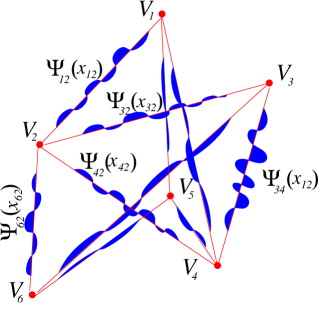
FIG. 1.: Quantum graph: a quantum particle moves along the bonds of a generic graph and scatters at its vertices.

The bonds $B_{ij}$ of the graph may be equipped with potentials $U_{ij}$. We refer to these potentials as bond potentials or the dressing of the graph bonds. The parameters determining the strength and the shape of the bond potentials are referred to as dressing parameters. In what follows the bond potentials are considered to be scaling potentials, $U_{ij}=\lambda_{ij}E$, $\lambda_{ij}=\lambda_{ji}=const$. The physical meaning and the reason for introducing the scaling assumption are discussed in [7, 8, 9, 10]. In addition, in Sec. VII, we present a physical analogue system of scaling quantum graphs, a network of taut strings, which has the same spectral equation as scaling quantum graphs. The string system is an example of a naturally scaling system. In a more general context one can consider the scaling assumption as a tool which allows to avoid unnecessary mathematical complications. For most physical systems scaling can be achieved, even experimentally [13], by an appropriate choice of parameters. We also define $E=k^{2}$ since for the discussion below it is frequently more convenient to work with $k$ than to work with $E$.

For $\hbar=0$ quantum graphs produce strongly stochastic (mixing) classical counterparts – a classical particle moving on the same one-dimensional network, scattering randomly on its vertices [1, 2, 14, 15, 16]. We use the word stochastic to characterize the classical dynamics of the particle on the graph since classically the scattering at the vertices is not a deterministic process as required for deterministic chaos[17], but a random, stochastic process, where the classical scattering probabilities are determined directly from the quantum dynamics in the limit $\hbar\rightarrow 0$ [18].

Despite the apparent simplicity of quantum graphs, their behavior exhibits many familiar features of classically chaotic systems. Examples are the exponential proliferation of classical periodic orbits and the approximate Wignerian statistics of nearest-neighbor spacings [1, 2] (see also Sec. V). As a result quantum graphs are quantum stochastic systems, which mimic closely the behavior of quantum chaotic systems. It is therefore very interesting that despite their classical stochasticity and despite many familiar phenomenological features of quantum chaos exhibited in the quantum regime, the spectral problem for scaling quantum graphs turns out to be explicitly solvable [11, 19].

Let us first outline the solution for a particular class of scaling quantum graphs, called regular in [7, 8, 9, 10]. We note that the term “regular” as used here refers to the regular behavior of the spectrum of the corresponding quantum graphs and has nothing to do with regular graphs as defined in graph theory [20], e.g. graphs with a fixed coordination number. A case in point is the recent paper by Severini and Tanner [21] where the term “regular quantum graphs” refers to quantum graphs with a special graph topology.

For regular quantum graphs there exists a set of $k$-intervals $I_{n}$, each of which contains precisely one momentum eigenvalue $k_{n}$ (see Appendix A). The end points $\hat{k}_{n}$ of these intervals, $I_{n}=\left[\hat{k}_{n-1},\hat{k}_{n}\right]$, form a periodic set,

$$\hat{k}_{n}=\kappa_{1}n+\kappa_{2},$$ (1)

where the constants $\kappa_{1},\kappa_{2}$ are determined explicitly in terms of the parameters of the quantum graph. Clearly, the points $\hat{k}_{n}$ separate the eigenvalues $k_{n}$ from each other, and are therefore called separators (see Sec. IV).

As soon as the separators $\hat{k}_{n}$ and the density of states $\rho(k)$ are known, an explicit expression for the energy eigenvalues of a given quantum graph is obtained either by first computing the momentum eigenvalues

$$k_{n}=\int_{\hat{k}_{n-1}}^{\hat{k}_{n}}\rho(k)\,kdk,$$ (2)

and then using $E_{n}=k_{n}^{2}$, or by computing $E_{n}$ directly as

$$E_{n}=\int_{\hat{E}_{n-1}}^{\hat{E}_{n}}\rho(E)\,EdE,$$ (3)

where $\hat{E}_{n}=\hat{k}_{n}^{2}$, $\rho(E)dE=\rho(k)dk$. An explicit periodic-orbit expansion of the density of states $\rho(k)$ is given by [7, 8]

$$\rho(k)\equiv\sum_{n}\delta(k-k_{n})=\frac{S_{0}}{\pi}+\mathop{\rm Re}\frac{1}{\pi}\sum_{p}S_{p}^{0}\sum_{\nu=1}^{\infty}A_{p}^{\nu}e^{i\nu S^{0}_{p}k},$$ (4)

where $S^{0}_{p}$, and $A_{p}$ are correspondingly the reduced action lengths and the weight factors of the prime periodic orbits labeled by $p$, $\nu$ is the multiple traversal index, and $S_{0}$ is the total reduced action length of the graph [9]. The constant term in the expansion (4) of $\rho$ shows that $\kappa_{1}$ in Eq. (1) is given by $\kappa_{1}=\pi/S_{0}$. In order to illustrate the construction of explicit spectral formulas we assume, for simplicity, that $\kappa_{2}=1/2$ and all $A_{p}$ are real. Both assumptions hold for a large class of regular quantum graphs. If we now use the expansion (4) in Eq. (3) we arrive at the following exact, explicit periodic-orbit expansion of the individual energy levels of the corresponding regular quantum graphs:

$$E_{n} = \frac{\pi^{2}}{S_{0}^{2}}\left(n^{2}+\frac{1}{12}\right)-\frac{4\pi n}{S_{0}^{2}}\mathop{\rm Im}\sum_{p,\nu}\frac{A_{p}^{\nu}}{\omega_{p}\nu^{2}}\sin\left(\frac{\omega_{p}\nu}{2}\right)\,e^{in\omega_{p}\nu}$$ (6)

$$-\frac{4\pi}{S_{0}^{2}}\mathop{\rm Re}\sum_{p,\nu}\frac{A_{p}^{\nu}}{\nu^{3}\omega_{p}^{2}}\left[\sin\left(\frac{\omega_{p}\nu}{2}\right)-\left(\frac{\omega_{p}\nu}{2}\right)\cos\left(\frac{\omega_{p}\nu}{2}\right)\right]\,e^{in\omega_{p}\nu},$$

where $\omega_{p}=\pi S_{p}^{0}/S_{0}$. Therefore, according to (6), the index $n$ that counts the separators $\hat{k}_{n}$ of the regular quantum graph, is a quantum number in the sense that it explicitly enumerates the physical eigenstates. In this respect, the explicit formulas for the quantum energy levels $E_{n}$ of these systems are analogous to the well-known Einstein-Brillouin-Keller (EBK) quantization formulas for integrable systems [4, 5, 6]. This is a very interesting fact from the point of view of the semiclassical periodic-orbit quantization theory. In this respect, the regular quantum graphs represent curious hybrids of classical stochasticity and quantum spectral solvability.

However, the systems for which the expansion (6) is valid, represent a very special class of quantum graphs. Just how special such “spectral regularity” is, can be illustrated in terms of the behavior of the corresponding spectral staircase function,

$$N(E)=\sum_{n}\theta(E-E_{n}),$$ (7)

where $\theta$ is the unit step function defined as

$$\theta(x)=\cases{0,&for $x<0$,\cr 1/2,&for $x=0$,\cr 1,&for $x>0$.\cr}$$ (8)

It was shown in [7, 10], that for the regular systems, the average spectral staircase (Weyl’s average),

$$\bar{N}(E)=\frac{S_{0}}{\pi}\sqrt{E}+\bar{N}(0),$$ (9)

has the piercing property, i.e. it intersects every stair step of the spectral staircase function $N(E)$, as illustrated in Fig. 2.

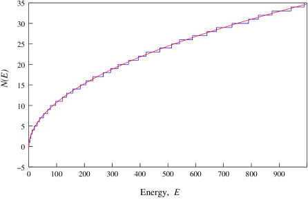
FIG. 2.: Piercing property of the regular quantum graphs. The spectral staircase function of a regular quantum graph is pierced by its average $\bar{N}(E)$.

If a quantum system has the piercing property, there exists exactly one intersection point $\hat{E}_{n-1}$, between every two neighboring energy levels $E_{n-1}<E_{n}$,

$$N(\hat{E}_{n-1})=\bar{N}(\hat{E}_{n-1}),\ \ E_{n-1}<\hat{E}_{n-1}<E_{n},\ \ \ n=1,2,\ldots\,\,.$$ (10)

The $\hat{E}_{n}$ thus defined may serve as separators for the quantum energy spectrum. As shown in Fig. 2 the piercing-average requirement (10) is indeed quite restrictive. Consequently, regular quantum graphs form a relatively small subset of quantum graphs. As demonstrated in [10, 22], only a few graph topologies (for instance linear chains) admit a regular regime for an appropriate choice of network parameters. As an example, a four-vertex linear-chain quantum graph (see inset of Fig. 3), which is characterized by the values of the two reflection coefficients $r_{2}$ and $r_{3}$ at the two middle vertices $V_{2}$ and $V_{3}$, is in the regular regime if these parameters fall into the shaded region shown in Fig. 3.

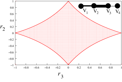
FIG. 3.: The parameter space of the four-vertex linear graph. The shaded region corresponds to the regular regime.

The majority of scaling quantum graphs do not admit regular regimes. Hence it is intriguing to understand the spectral behavior of irregular quantum graphs, i.e. those for which the piercing-average condition (10) is violated.

III Spectral equation

In order to set the stage for the following discussion, let us recall some general definitions and properties of quantum graphs. As mentioned in the introduction, a quantum graph [1, 2, 3] consists of a quantum particle moving on a one-dimensional network of $N_{B}$ bonds connecting $N_{V}$ vertices (Fig. 1). Every bond $B_{ij}$ which connects the vertices $V_{i}$ and $V_{j}$, carries a solution of the Schrödinger equation, $\hat{H}\psi_{n}=E_{n}\psi_{n}$. The length of the bonds is denoted by $L_{ij}$. With the constant scaled potentials $U_{ij}=\lambda_{ij}E$ defined on the bonds of the graph, the Schrödinger equation is

$$\frac{d^{2}}{dx^{2}_{ij}}\psi_{ij}(x)+\beta_{ij}^{2}E\psi_{ij}(x)=0,$$ (11)

where $\beta_{ij}=\pm\sqrt{1-\lambda_{ij}}$.

Below we shall assume for simplicity that the energy $E$ is kept above the maximal scaled potential height, i.e. $\lambda_{ij}<1$, $i,j=1,...,N_{V}$, so that tunneling solutions are excluded and the general solution of Eq. (11) on the bond $B_{ij}$ is

$$\psi_{ij}(x)=a_{ij}e^{-ik\beta_{ij}x_{ij}}+b_{ij}e^{ik\beta_{ij}x_{ij}}.$$ (12)

The quantization conditions for quantum graphs are the result of the requirement that the solutions (12) must satisfy the continuity and the current conservation conditions at every vertex $V_{i}$. The procedure of imposing the boundary conditions can be reformulated in terms of an auxiliary problem of quantum scattering on the vertices of the graph [2, 10, 14], which provides an elegant solution of the graph quantization problem. As shown in [2, 10, 14] the consistency of the complete set of boundary conditions at all vertices yields the spectral equation

$$\Delta(k)=\det\left[1-S(k)\right]=0,$$ (13)

where $S(k)$ is a $2N_{B}\times 2N_{B}$ unitary (scattering) matrix [2, 10, 14],

$$S_{IJ}(k)=t_{IJ}e^{i\beta_{I}L_{I}k}.$$ (14)

Here the capital indices $I$, $J$ are used to denote the directed bonds, $I,J=1,2,...,2N_{B}$. We denote by $I^{\prime}$ the time-reversed bond of $I$. The elements $t_{IJ}$ (discussed in detail in [10]) have the meaning of transmission (reflection) amplitudes for transitions between the (directed) bonds $I$ and $J$. Transmission occurs if $I$ and $J$ are connected and $J\neq I^{\prime}$. If $I$ and $J$ are not connected, we have $t_{IJ}=0$. An example here is $t_{II}=0$ for all $I$. For $J=I^{\prime}$ the matrix element $t_{IJ}$ has the meaning of a reflection amplitude [2, 9, 10, 14]. Due to the scaling condition, the $t_{IJ}$’s are constant ($k$-independent) parameters.

For conventional quantum graphs without potential dressing the connection between the coefficients $t_{IJ}$ and the expansion coefficients $A_{p}$ in Eqs. (4) and (6) was established early on in the seminal literature on quantum graphs, e.g. in Refs. [1, 2]. Later it was shown to hold also in the case of dressed, scaling quantum graphs [15]. Each transition of an orbit $p$ from a bond $I$ to $J$ contributes the factor $t_{IJ}$ to the weight $A_{p}$ of the orbit, so that

$$A_{p}=\prod_{\{p\}}t_{IJ},$$ (15)

where the product is taken over the sequence of bonds traced.

Note that the phases of the exponentials in Eq. (14) coincide with the classical actions associated with the particle path traversing the bond $B_{I}$,

$$S_{I}(k)=\beta_{I}L_{I}k.$$ (16)

The spectral determinant (13) can be written in the form

$$\Delta(k)=e^{i\Theta_{0}(k)}\,\Delta_{R}(k),$$ (17)

where $\Delta_{R}(k)$ is the (real) modulus of $\Delta(k)$ and $\Theta_{0}(k)$ is its phase. The phase is given by [9]

$$\Theta_{0}(k)=\frac{1}{2}\ln\det S=S_{0}k-\pi\gamma_{0},$$ (18)

where $S_{0}$, the total reduced action length as introduced in Eq. (4), is given explicitly by

$$S_{0}={1\over 2}\sum_{I=1}^{2N_{B}}L_{I}\beta_{I}$$ (19)

and $\gamma_{0}$ is a constant phase. The modulus is given by [9]

$$\Delta_{R}(k)=\cos\left(S_{0}k-\pi\gamma_{0}\right)-\sum_{i=1}^{N_{\Gamma}}a_{i}\cos(S_{i}k-\pi\gamma_{i}),$$ (20)

where $a_{i}$ are constant coefficients, $\gamma_{i}$ are constant phases, $N_{\Gamma}$ is the number of harmonic terms in the sum of Eq. (20) and the frequencies $S_{i}$ are linear combinations of the reduced classical bond action lengths $S_{I}^{0}=\beta_{I}L_{I}$. $S_{0}$ is the largest frequency in Eq. (20), i.e. $S_{i}<S_{0}$, $i=1\ldots N_{\Gamma}$. This fact will be of crucial importance below.

The spectrum of the quantum graph is obtained from the equation

$$\Delta_{R}(k)=0.$$ (21)

In Appendix A we prove that if the coefficients of the characteristic function $\Phi(k)$ of the graph,

$$\Phi(k)\equiv\sum_{i=1}^{N_{\Gamma}}a_{i}\cos(S_{i}k-\pi\gamma_{i}),$$ (22)

satisfy the condition

$$\sum_{i=1}^{N_{\Gamma}}\left|a_{i}\right|\equiv\alpha<1,$$ (23)

precisely one solution $k_{n}$ of Eq. (21) can be found between each two sequential separators

$$\hat{k}_{n}=\frac{\pi}{S_{0}}\left(n+\gamma_{0}+\mu+1\right),$$ (24)

where $\mu$, an integer, is to be adjusted such that $k_{1}<\hat{k}_{1}<k_{2}$. This is the case, e.g. for a two-bond graph (Fig. 4) with the bond lengths $L_{1}$ and $L_{2}$, for which the spectral equation is

$$\sin(S_{0}k)-r\sin(S_{1}k)=0.$$ (25)

Here $S_{0}=L_{1}\beta_{1}+L_{2}\beta_{2}$, $S_{1}=L_{1}\beta_{1}-L_{2}\beta_{2}$, and $r$ is a constant positive reflection coefficient at the vertex $V_{2}$ between the two bonds. Since $|r|<1$, the condition (23) is satisfied and hence this graph is always regular.

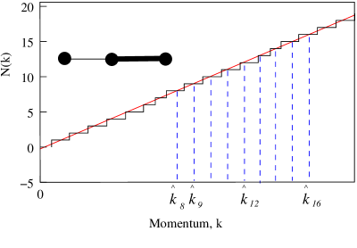
FIG. 4.: The three-vertex linear graph (inset) and the corresponding staircase function. The intersections between $\bar{N}(k)$ and $N(k)$ correspond to the separating points $\hat{k}_{n}$.

In this case every step of the spectral staircase function (7) is pierced by its average (Fig. 4), or equivalently, every interval $I_{n}=[\hat{k}_{n-1},\hat{k}_{n}]$ contains precisely one quantum eigenvalue of the momentum. This spectral regularity is the key for obtaining the explicit harmonic expansion for each individual root of the spectral determinant (13). In general, however, the regularity condition (23) does not hold and hence the principle “one root per interval $I_{n}$” (see Appendix A) is violated. This is illustrated in Fig. 5, which shows the behavior of the spectral staircase for the four-vertex linear chain in two different dynamical regimes. The spectral staircase on the right corresponds to a case in which the parameters $r_{2}$ and $r_{3}$ fall outside of the shaded regularity region in Fig. 3.

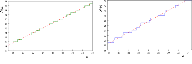
FIG. 5.: The staircase and the average $\bar{N}(k)$ for the four-vertex linear graph in a regular (left) and in an irregular (right) regime.

Hence, in order to proceed with an analysis similar to the one for regular quantum graphs, one needs to find a set of separating points that “bootstrap” the spectrum, and allow us to integrate around each delta-peak of $\rho(k)$, as in Eq. (2).

IV Separators

What is the set of points that can be used as separators for a generic quantum graph? Since the points $k_{n}$ that need to be separated, are the zeros of the spectral determinant $\Delta_{R}(k)$, one can invoke an elementary, classic theorem [23], which states that between every two roots of a real, continuous, differentiable function there exists an extremum point. Moreover, extending $\Delta_{R}(k)$ into the complex plane, $\Delta_{R}(k)\rightarrow\Delta(z)$, and using the Hadamard representation of the resulting entire function $\Delta(z)$,

$$\Delta(z)=e^{i(S_{0}z-\pi\gamma_{0})}z^{q}\prod_{n}\left(1-\frac{z}{k_{n}}\right)e^{\frac{z}{k_{n}}},$$ (26)

where $q\geq 0$ is the multiplicity of the root $k_{n}=0$, and all the roots $k_{n}$ are assumed to be real as required, since $\Delta_{R}(k)$ is derived from a Hermitian eigenvalue problem, one can show [24, 25] that there is exactly one zero between every two neighboring extrema of $\Delta_{R}(k)$, i.e. that the zeros and the extrema interlace and “extra wiggles” such as, e.g., illustrated by the dashed line in Fig. 6, are not possible. Hence the locations of extrema may be used as the separating points for bootstrapping the physical spectrum.

FIG. 6.: The interlacing sequence of roots and extrema of the spectral determinant. The dashed line represents the forbidden “extra wiggles”.

Strictly speaking, all this works only for simple roots of $\Delta(z)$, which is the generic case. Multiple roots may, and in special cases do, occur. But as explained in Refs. [11, 19], these cases are trivial to deal with. In such a case the separators and the spectral points are degenerate and no further computation is necessary.

Is it any easier to obtain the extrema of $\Delta_{R}(k)$ than to obtain its roots? Interestingly, looking for the answer to this question provides us with a complete scheme for establishing a hierarchy of quantum graphs according to their spectral irregularity. Let us examine this question more closely.

The equation $\Delta_{R}^{\prime}(k)=0$ that defines the extrema of $\Delta_{R}(k)$ is

$$\sin\left(S_{0}k-\pi\gamma_{0}\right)-\sum_{i=1}^{N_{\Gamma}}a_{i}\epsilon_{i}\sin(S_{i}k-\pi\gamma_{i})=0,$$ (27)

where

$$\epsilon_{i}=\frac{S_{i}}{S_{0}}<1.$$ (28)

Note that this is the same type of trigonometric polynomial as the original spectral equation (21) (with a shifted phase $\gamma_{0}$), with the new characteristic function

$$\Phi^{(1)}(k)\equiv\sum_{i=1}^{N_{\Gamma}}a_{i}\epsilon_{i}\sin(S_{i}k-\pi\gamma_{i}).$$ (29)

However, compared to the original $\Phi(k)$ of Eq. (22), this function has certainly a better chance of satisfying the regularity condition (23), because the absolute values of the coefficients $a_{i}$ have been decreased by the factors $\epsilon_{i}<1$, i.e.

$$a_{i}\rightarrow a_{i}\epsilon_{i}.$$ (30)

Let us assume that for a certain irregular graph with $\sum_{i=1}^{N_{\Gamma}}\left|a_{i}\right|>1$, the new characteristic function $\Phi^{(1)}(k)$ actually does satisfy the regularity condition (23), i.e.

$$\sum_{i=1}^{N_{\Gamma}}\left|a_{i}\epsilon_{i}\right|<1.$$ (31)

According to the results of Secs. II and III this means that the zeros of $\Delta_{R}^{\prime}(k)$ (the extremal points of $\Delta_{R}(k)$) can be separated from each other by the periodic sequence of separators (24), i.e. that there exists exactly one extremum of $\Delta_{R}(k)$ between every two points $\hat{k}_{n}$. For functions of the type (26) the converse statement is also true [24, 25], i.e. there exists a root of $\Delta_{R}(k)$ between every two extrema of $\Delta_{R}(k)$. This suggests a direct strategy for obtaining the roots of Eq. (21). First, as mentioned above, we note that the spectral equation for $\Delta_{R}^{\prime}(k)$ can be written in the form

$$\Delta_{R}^{\prime}(k)=\sum_{j=0}^{N_{\Gamma}}C_{j}\cos(S_{j}k+\varphi_{j})=0,$$ (32)

where $C_{j}$ and $\varphi_{j}$ are constants. From this we obtain the following explicit formula for the density-of-extremas functional $\rho^{(1)}(k)$

$$\rho^{(1)}(k)=|\Delta_{R}^{\prime\prime}(k)|\,\delta(\Delta_{R}^{\prime}(k))=|\Delta_{R}^{\prime\prime}(k)|\,{1\over 2\pi}\,\int_{-\infty}^{\infty}\,e^{iy\Delta_{R}^{\prime}(k)}\,dy=$$

$$|\Delta_{R}^{\prime\prime}(k)|\,{1\over 2\pi}\sum_{n_{0}=-\infty}^{\infty}\ldots\sum_{n_{N_{\Gamma}}=-\infty}^{\infty}\left[\int_{-\infty}^{\infty}\prod_{j=0}^{N_{\Gamma}}J_{n_{j}}(yC_{j})\,dy\right]\,\exp\left\{i\sum_{l=0}^{N_{\Gamma}}n_{l}[S_{l}k+\varphi_{l}]\right\},$$ (33)

where the $J_{n}$ are Bessel functions of the first kind [26], and the integrals in Eq. (33) converge for $C_{j}\neq 0$. Now, using the expansion (33) together with the periodic separators (24), one obtains the separating points $\hat{k}_{n}^{(0)}$ for the roots $k_{n}$ of $\Delta_{R}(k)$, via

$$\hat{k}^{(0)}_{n}=\int_{\hat{k}_{n-1}^{(1)}}^{\hat{k}_{n}^{(1)}}\rho^{(1)}(k)\,k\,dk.$$ (34)

Here we used the notation $\hat{k}_{n}^{(1)}$ for the periodic separators (24), for future convenience. Following this step, using the separators $\hat{k}_{n}^{(0)}$ obtained in Eq. (34), we find the roots $k_{n}$ of the spectral equation via

$$k_{n}=\int_{\hat{k}_{n-1}^{(0)}}^{\hat{k}_{n}^{(0)}}\rho^{(0)}(k)\,k\,dk,$$ (35)

where the notation $\rho^{(0)}(k)$ was used for the density of states $\rho(k)$.

For the case of the four-vertex linear graph, this situation is again illustrated in Fig. 3, in which it is now assumed that the differentiated equation (27) satisfies the regularity condition all through the domain $-1\leq r_{2},r_{3}\leq 1$. This would be the case, e.g., if the bond action lengths are chosen to be $S_{1}^{0}=0.25$, $S_{2}^{0}=0.45$, and $S_{3}^{0}=1-S_{1}^{0}-S_{2}^{0}$. For this case one can immediately verify that the spectral equation of the four-vertex linear chain,

$$\sin(S_{0}k)=r_{3}\sin(S_{1}^{0}k+S_{2}^{0}k-S_{3}^{0}k)-r_{2}r_{3}\sin(S_{1}^{0}k-S_{2}^{0}k+S_{3}^{0}k)$$ (36)

$$+r_{2}\sin(S_{1}^{0}k-S_{2}^{0}k-S_{3}^{0}k),$$ (37)

is irregular outside of the region $|r_{3}|+|r_{2}r_{3}|+|r_{2}|<1$, but the coefficients of the differentiated equation satisfy the regularity condition (23).

Clearly this strategy can be applied in the general case. If the differentiated equation (27) is not of the regular type, one can differentiate the spectral equation (21) as many times as it is necessary to obtain an equation of regular type at the $m$-th step. Indeed, the $l$-th derivative of the spectral equation is

$$\Delta_{R}^{(l)}(k)=\cos\left(S_{0}k-\pi\gamma_{0}+\frac{\pi l}{2}\right)-\sum_{i=1}^{N_{\Gamma}}a_{i}\epsilon_{i}^{l}\cos\left(S_{i}k-\pi\gamma_{i}+\frac{\pi l}{2}\right).$$ (38)

Obviously, since all $\epsilon_{i}$’s are smaller than 1, we eventually (after a finite number $m$ of steps) arrive at an equation that satisfies the regularity condition (23),

$$\sum_{i=1}^{N_{\Gamma}}\left|a_{i}\epsilon_{i}^{m}\right|<1.$$ (39)

An upper bound for $m$ is easily established. We have $m\leq-\ln(\sum_{i=1}^{N_{\Gamma}}|a_{i}|)/\ln(\max_{i}\epsilon_{i})$. Then, once the condition (39) for the $m$-th derivative of its spectral determinant is satisfied, its zeros are separated from each other by a periodic sequence of points,

$$\hat{k}_{n}^{(m)}=\frac{\pi}{S_{0}}\left(n+\gamma_{0}+\mu+1\right)$$ (40)

as in Eq. (24). Using the density $\rho^{(m)}(k)$ of zeros of $\Delta_{R}^{(m)}(k)$, which is obtained explicitly in complete analogy with Eq. (33), we can evaluate the zeros themselves as

$$\hat{k}^{(m-1)}_{n}=\int_{\hat{k}_{n-1}^{(m)}}^{\hat{k}_{n}^{(m)}}\rho^{(m)}(k)\,k\,dk.$$ (41)

Obviously, these points are now the extrema of $\Delta_{R}^{(m-1)}(k)$, and moreover, since there is exactly one root of $\Delta_{R}^{(m)}(k)$ between any two neighboring points $\hat{k}_{n}^{(m)}$, $\Delta_{R}^{(m-1)}(k)$ has no extrema other than the ones obtained in Eq. (41).

The newly obtained extrema of $\Delta_{R}^{(m-1)}(k)$ separate its zeros from each other, and hence serve as the separators for the roots of $\Delta_{R}^{(m-1)}(k)$. As a consequence, we can now find all the roots of $\Delta_{R}^{(m-1)}(k)$ by using Eq. (41) recursively until we arrive at the $0$-th level to obtain the roots $k_{n}$ of the original spectral determinant. This solves the problem of obtaining the energy spectrum of any scaling quantum graph.

It is important to realize that a quantum graph of a certain topology can still have different degrees of irregularity depending on the network’s bond lengths and dressing parameters (for instance the values of the bond potentials). This point is easily illustrated by once more using the example of the four-vertex linear chain. Although the regularity region for this graph is always the same, the surrounding blank region in Fig. 3, which corresponds to the irregular regime, now acquires structure. Figure 7 shows the spectral diagram for the four-vertex linear-chain graph for two different sets of graph parameters, corresponding to two different irregularity regimes.

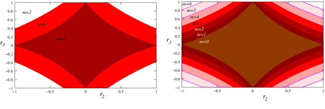
FIG. 7.: The spectral regime diagram of the four-vertex linear-chain quantum graph. The bond-action lengths are chosen to be $S_{1}^{0}=0.2$, $S_{2}^{0}=0.6565$, $S_{3}^{0}=1-S_{1}^{0}-S_{2}^{0}$ (left panel), and $S_{1}^{0}=0.1$, $S_{2}^{0}=0.8565$, $S_{3}^{0}=1-S_{1}^{0}-S_{2}^{0}$ (right panel) resulting in a maximum degree of irregularity of $m=2$ (left panel) and $m=6$ (right panel).

The central diamond-shaped regions ($m=0$) in Fig. 7 are the same as in Fig. 3 and correspond to the same regularity region as in Fig. 3. The outer layers of the regular region in Fig. 7 correspond to parameter values that guarantee first ($m=1$), second ($m=2$), …, degree of irregularity.

V Spectral statistics

It is well known that the statistical properties of the spectra of generic quantum graphs are well described by Random Matrix Theory (RMT) [1, 2]. In particular, the numerically obtained nearest-neighbor distribution $P(s)$ of the normalized spacings $s$ [5] of the eigenvalues of highly connected quantum graphs follows closely the profile of the Gaussian random matrix ensembles, both in the presence of the time reversal symmetry (GOE), where the nearest-neighbor distribution is given by [5]

$$P_{\rm GOE}(s)={\pi\over 2}\,s\,\exp(-s^{2}\pi/4)$$ (42)

and in the absence of it (GUE), where the nearest-neighbor distribution is given by

$$P_{\rm GUE}(s)={32\over\pi^{2}}\,s^{2}\,\exp(-4s^{2}/\pi).$$ (43)

This circumstance is one of the most important motivations for studying quantum graphs in the context of quantum chaos theory. In particular it is hoped to gain more insight into the connection between chaos and random matrix theory and, if possible, to prove the Bohigas-Giannoni-Schmit conjecture [27, 28], which states that, generically, the spectrum of quantum Hamiltonian systems chaotic in the classical limit should conform with the spectral properties of the random matrix ensembles.

However, the exact results presented above show that for quantum graphs with a finite number of bonds and vertices (finite quantum graphs) the correspondence with the nearest-neighbor distributions (42) and (43), respectively, can only be approximate. Indeed, the existence of root separators implies that the eigenvalues of the momentum, $k_{n}$, will always be confined within the root cells, $k_{n}\in[\hat{k}_{n-1},\hat{k}_{n}]$. Hence, for finite quantum graphs, even though they may be highly connected, the statistical distribution $P(s)$ of the nearest neighbor separations, $s_{n}=k_{n}-k_{n-1}$, will be restricted to the finite domain $0<s<s_{max}$, and will not have the characteristic long tail of the nearest-neighbor distributions (42) and (43), respectively. This general property of the spectra of scaling quantum graphs also follows from the fact that their spectral function, $\Delta_{R}(k)$, is an almost periodic function of the momentum, and hence its zeros form an almost periodic set [29]. It is clear, therefore, that the distances between neighboring points of this set are bounded, i.e. $s<s_{max}$, and $P(s)$ is zero for $s>s_{max}$. These observations, of course, do not preclude the possibility that certain finite, highly connected quantum graphs are well, or indeed even exactly described by the finite matrix ensembles [5].

However, the higher the degree of irregularity of a quantum graph, the larger $s_{max}$. Going upwards in the “hierarchy of separators” leads to an increase in the allowed nearest neighbor spacings, since the maximal possible distance between neighboring separators grows by one unit of mean spacing when going from complexity level $m-1$ to complexity level $m$. The mechanism for the increase of the allowed maximal nearest-neighbors spacing as a function of $m$ is illustrated in Fig. 8.

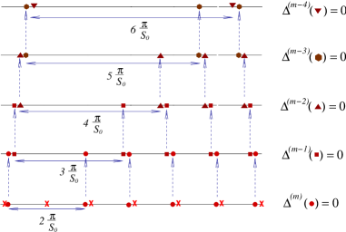
FIG. 8.: Increase of the maximally allowed nearest-neighbor separation as a function of $m$, generated by the hierarchy of the separators. At the regular level ($\Delta^{(m)}$), the periodically spaced separators $\hat{k}_{n}^{(m)}$ (marked by $\times$) separate the roots of $\Delta_{R}^{(m)}(k_{n}^{(m)})=0$ (full circles). Their maximally allowed distance is $2\frac{\pi}{S_{0}}$. The second order separators (the roots of $\Delta_{R}^{(m-1)}(k_{n}^{(m-1)})=0$), may be maximally as far as $3\frac{\pi}{S_{0}}$ apart, etc. The higher the hierarchy of the separator, the larger the maximally allowed spacing of nearest neighbors.

Figure 8 also shows that the roots of a spectral equation $\Delta_{R}(k)=0$ with irregularity degree $m$, may be no more than $(m+1)\pi/S_{0}$ apart. This provides a simple rule for finding an upper limit for $s_{max}$,

$$s_{max}^{(m)}\leq d_{max}^{(m)}=\frac{\pi}{S_{0}}(m+1).$$ (44)

Clearly, the possibility of having large separations between the nearest neighbors is necessary for producing a statistical distribution for $s_{n}=k_{n}-k_{n-1}$ that resembles a Wignerian distribution profile, similar to the ones which were numerically obtained in Ref. [2].

On the other hand, it is essential to realize that a high irregularity degree $m$ is not enough to guarantee Wignerian-like statistics of the nearest neighbor spacings. A simple numerical experiment with the spectral equation (37) shows that the separations between nearest neighbors do not necessarily assume the largest possible values (44). Hence the degree of irregularity indeed provides only an upper limit for the nearest-neighbor separations, and does not determine by itself their actual values.

For example, the dressing parameters of a quantum network can be changed continuously so that the system undergoes a transition from an irregularity $m$ regime to an irregularity $m+1$ regime. As this transition happens, the roots of the spectral equation do not respond to produce an abrupt increase of the nearest-neighbor separations by $\pi/S_{0}$. Instead, the maximal nearest-neighbor separation increases smoothly as a function of the dressing parameters.

There is a convenient way to illustrate this increase for the four-vertex chain network, using the structure of its spectral regime diagram (Fig. 7). As shown in Fig. 7, the parameter regions that correspond to different irregularity degrees for this graph form a system of nested diamond shapes, with high irregularity regimes concentrating toward the corners of the diagram. A specific set of the action length values, $S_{1}^{0}$, $S_{2}^{0}$, $S_{3}^{0}$, defines the frequencies in (37) and hence the maximal irregularity degree $m_{max}$, i.e. the total number of diamond-shaped regions, while a choice of the reflection coefficients, $r_{2}$ and $r_{3}$, puts the system onto a particular point in the diagram. Hence, one can study the effect of increasing irregularity by traversing the spectral regime diagram from its center ($r_{2}=r_{3}=0$) to one of the corners (say, $r_{2}=r_{3}=1$) along the line $r_{2}=r_{3}=r$, $0\leq r\leq 1$. For each value of $r=r_{2}=r_{3}$ that corresponds to a particular irregularity degree, $m$, one can obtain numerically the maximal separation distance, $s_{max}$, between the nearest neighbors, and then follow its change as $m$ increases.

In addition to the maximal separation $s_{max}$ there also exists a minimal separation $s_{min}$. The vertical bars in Fig. 9 represent the possible range of nearest-neighbor spacings $s_{min}\leq s\leq s_{max}$ for given $m$. Clearly, the maximal root separation is increasing with growing $m$. However the increase is slower than the one given by the linear estimate $d_{max}^{(m)}$ in Eq. (44).

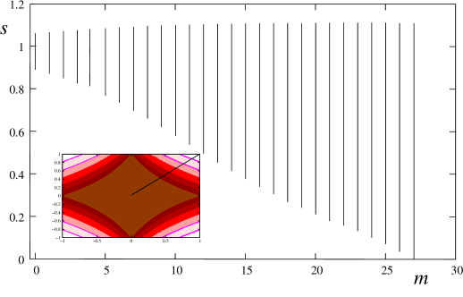
FIG. 9.: Range of nearest-neighbor spacings $s/\pi$ as a function of the irregularity degree $m$ for the four-vertex chain. The maximal separation was obtained based on the roots found in the interval $0\leq k\leq\pi 10,000$ in each $m$ regime. The bond action lengths are $S_{1}^{0}=0.1$, $S_{2}^{0}=0.8999$, $S_{3}^{0}=0.0001$, which produce a maximal irregularity degree of $m_{max}=27$.

Since the spectral equation (37) is an almost periodic function, the maximal root separation found on a sufficiently large finite interval of the momenta (large compared to the smallest almost-period of the function (37)) is indeed the maximal root separation produced by this function on arbitrary intervals.

It is also important to notice that the maximal nearest-neighbor separations $s_{max}$ can be different for two graphs with the same degree of irregularity. Moreover, two quantum graphs with the same irregularity degree may have completely different spectral statistics. This can be seen from comparing the cases of the topologically simple four-vertex chain graph with the fully connected four-vertex quadrangle. The spectral statistics provided by the latter example were previously discussed in Ref. [2]. It was shown that the nearest-neighbor distribution follows quite closely the anticipated Wignerian shape (both in the GOE and in the GUE cases).

The analysis of the spectral equation of a four-vertex quadrangle with no bond potentials and comparable bond lengths (the case considered in Ref. [2]) produces an irregularity degree that usually does not exceed $m\approx 25$. This level of irregularity can be easily achieved by the four-vertex chain, which, unlike the quadrangle, does not produce the characteristic Wignerian distribution profile. The distribution produced by a four-vertex chain in different irregularity regimes is shown in Fig. 10.

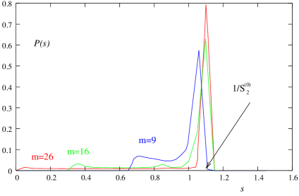
FIG. 10.: Nearest-neighbor spacing probability distributions for the eigenvalues of the four-vertex linear-chain quantum graph with bond action lengths $S_{1}^{0}=0.1$, $S_{2}^{0}=0.8999$, $S_{3}^{0}=0.0001$, in different regimes of irregularity $m$ as a function of spacing $s$ (in units of $\pi$). The distribution profile is not Wignerian. The higher the irregularity index $m$, the higher the peak of the distribution around $s/\pi\approx 1/S_{2}^{0}$.

Some general features of these distribution curves can be easily explained with the help of elementary quantum-mechanical arguments applied to the four-vertex chain. Indeed, it is clear from Fig. 7, that high irregularity degree for a four-vertex chain can be achieved by selecting both reflection coefficients $|r_{2}|$ and $|r_{3}|$ close to $1$. Physically, such a choice implies that the bonds of the chain are essentially isolated, since the particle almost never transmits from one bond to another. This “bond decoupling” also manifests itself in the spectral properties of the system by the emergence of three apparent sub-sequences of eigenvalues, each associated with one of the “isolated-bond spectra”, $\pi n/S_{i}$. Hence, one would expect that in the case $|r_{2}|$, $|r_{3}|\approx 1$ the nearest-neighbor separations will mostly concentrate around the values determined by the inverse bond lengths, $s\approx|(\pi n_{i}/S_{i})-(\pi n_{j}/S_{j})|$, where $n_{i}$, $n_{j}$ are independent integers, rather than around a peak defined by the Wignerian distribution.

Overall, the results of the statistical analysis of the four-vertex chain spectrum show that both the small-$s$ and the large-$s$ ends of the $P(s)$ distribution profile change slowly with increasing irregularity degree. Even in the case of high irregularity degree, the behavior of the roots of Eq. (37) is too restricted by the simple analytical nature of Eq. (37) to exploit the possibility of getting as close to, or as far from, one another as is allowed by the hierarchy of the separators.

Since the irregularity hierarchy presented in previous sections is a completely general structure, the irregularity degree $m$ produced by this scheme is a very general index. However it does not, by itself, determine the spectral characteristics of a given quantum graph. While a small irregularity degree can be provided only by a few classes of graphs with relatively simple geometry, a large degree of irregularity can be shared by a wide variety of graphs, which include both the topologically simple ones (with appropriate dressings) and the topologically elaborate networks. It is natural, therefore, to expect that the statistical spectral properties produced by topologically simple graphs can differ from the ones produced by topologically complex networks, even if they are characterized by the same degree of irregularity $m$ in the sense of the bootstrapping scheme presented above.

The four-vertex chain graph, whose spectral equation (37) contains only four oscillating terms, is certainly too simple to produce random-matrix-like behavior, whereas a four-quadrangle, whose spectral equation written in the form (37) contains about 830 terms, is already sufficiently complex. This situation emphasizes the fact that the general phenomenological statement “classical chaos implies Wignerian statistics”, implicitly assumes sufficient complexity of the underlying classical system.

From the opposite perspective, it may be considered a curiosity that simple networks, such as the four-vertex chain, are capable of producing highly irregular spectra. It is interesting in this context to look for a more refined scheme that could distinguish between the complexity of the spectra provided by simple graphs (e.g. linear chains) and the spectra of more complicated networks, which are capable of producing random-matrix-like spectral statistics.

In this section we studied spectral properties of quantum graphs only as far as relevant in connection with our new “$m$-scheme”. Much more is known about the spectral properties of quantum graphs in general (see, e.g., [1, 2, 3, 21, 30, 31, 32, 33, 34, 35, 36]). In particular the thrust in the investigation of spectral properties nowadays is on understanding spectral correlation functions [1, 2, 3, 33, 34, 36] and even deriving explicit formuls for them [30, 35].

VI Lagrange’s inversion formula

The periodic orbit expansions presented in Sec. IV are not the only way to obtain the spectrum of regular quantum graphs explicitly. Lagrange’s inversion formula [37] offers an alternative route. Given an implicit equation of the form

$$x=a+w\varphi(x),$$ (45)

Lagrange’s inversion formula determines a root $x^{*}$ of Eq. (45) according to the explicit series expansion

$$x^{*}=a+\sum_{\nu=1}^{\infty}\,{w^{\nu}\over\nu!}\,{d^{\nu-1}\over dx^{\nu-1}}\,\varphi^{\nu}(x)\Big{|}_{a},$$ (46)

provided $\varphi(x)$ is analytic in an open interval $I$ containing $x^{*}$ and

$$|w|\ <\ \left|{x-a\over\varphi(x)}\right|\ \ \forall\ x\in I.$$ (47)

Since the regularity condition (23) ensures that the condition (47) is satisfied, we can use Lagrange’s inversion formula (46) to compute explicit solutions of regular quantum graphs.

In order to illustrate Lagrange’s inversion formula we will now apply it to the solution of Eq. (25). Defining $x=S_{0}k$, the $n$th root of Eq. (25) satisfies the implicit equation

$$x_{n}=\pi n+(-1)^{n}\,\arcsin[r\sin(\rho x_{n})],$$ (48)

where $\rho=S_{1}/S_{0}$ and $|\rho|<1$. Choosing $S_{0}=0.3+0.7/\sqrt{2}$, $S_{1}=0.3-0.7/\sqrt{2}$ and $r=(\sqrt{2}-1)/(\sqrt{2}+1)$, we obtain $x_{1}^{({\rm exact})}=3.26507\ldots$, $x_{10}^{({\rm exact})}=31.24664\ldots$ and $x_{100}^{({\rm exact})}=313.98697\ldots$. We now re-compute these values using the first two terms in the expansion (46). For our example they are given by

$$x_{n}^{(2)}=\pi n+\arcsin[r\sin(\rho\pi n)]\left\{(-1)^{n}+{r\rho\cos(\rho\pi n)\over\sqrt{1-r^{2}\sin^{2}(\rho\pi n)}}\right\}.$$ (49)

We obtain $x_{1}^{(2)}=3.26502\ldots$, $x_{10}^{(2)}=31.24650\ldots$ and $x_{100}^{(2)}=313.98681\ldots$, in very good agreement with $x_{1}^{({\rm exact})}$, $x_{10}^{({\rm exact})}$ and $x_{100}^{({\rm exact})}$.

Although both Eq. (6) and Eq. (46) are exact, and, judging from our example, Eq. (46) appears to converge very quickly, the main difference between Eq. (6) and Eq. (46) is that no physical insight is gained from Eq. (46), whereas Eq. (6) is tightly connected with the classical mechanics of the graph system providing, in the spirit of Feynman’s path integrals, an intuitively clear picture of the physical processes in terms of a superposition of amplitudes associated with classical periodic orbits.

VII Discussion

The first announcement of explicit periodic-orbit expansions of the spectrum of regular quantum graphs [8] was universally met with disbelief and puzzlement. It seemed impossible to obtain explicit solutions for a quantum system that had been shown to be an excellent model of quantum chaos [38] and, moreover, is completely stochastic in its classical limit [1]. However, we found that the rejection of our results was almost always based on the common misconception of the “unsolvability” of chaotic systems. We point out here that it is not true that classically chaotic systems are necessarily unsolvable. We hope that this insight will eliminate much of the reservations commonly expressed toward our results.

Examples of explicitly solvable chaotic systems are readily available. The shift map [39, 40],

$$x_{n+1}=(2x_{n})\ \ {\rm mod}\ 1,\ \ x_{n}\in{\rm{\bf R}},\ \ n=0,1,2,\ldots,$$ (50)

for instance, is “Bernoulli” [40], the strongest form of chaos. Nevertheless the shift map is readily solved explicitly,

$$x_{n}=(2^{n}\,x_{0})\ \ {\rm mod}\ 1,\ \ x_{n}\in{\rm{\bf R}},\ \ n=0,1,2,\ldots.$$ (51)

Another example is provided by the logistic mapping

$$x_{n+1}=\mu x_{n}(1-x_{n}),\ \ x_{n}\in[0,1],\ \ 0\leq\mu\leq 4,\ \ n=0,1,2,\ldots,$$ (52)

widely used in population dynamics [39, 40, 41]. For $\mu=4$ this mapping is equivalent with the shift map [42] and therefore completely chaotic. Yet an explicit solution, valid at $\mu=4$, is given by[42]:

$$x_{n}=\sin^{2}\left(2^{n}\arcsin\sqrt{x_{0}}\,\right),\ \ x_{0}\in[0,1].$$ (53)

Therefore, as far as classical chaos is concerned, there is no basis for the belief that classically chaotic systems do not allow for explicit analytical solutions. Our contribution in this paper is to show that scaling quantum graphs provide the first examples of explicitly solvable quantum stochastic systems.

In this paper we focussed on scaling quantum graphs mainly because of their mathematical simplicity. However, we will show now that for some physical systems the scaling property arises naturally as a consequence of the underlying physics.

Consider a taut string of length $L$, clamped at both ends, with a piecewise constant mass density $\mu(x)=\epsilon(x)\mu_{0}$, $\epsilon(x)=\epsilon_{i}$, $x_{i-1}<x<a_{i}$, $i=1,\ldots,4$, $a_{0}=0$, $a_{4}=L$, where $\mu_{0}$ is the average mass density of the string. This system contains the same physics as a four-vertex linear scaling quantum graph since the transverse acoustic excitations of the string satisfy the same spectral equation as a four-vertex linear scaling quantum graph. The reason is the following. For small transverse oscillations the string obeys the wave equation

$$\left[{d^{2}\over dx^{2}}+\omega^{2}{\mu(x)\over T}\right]\xi(x)=0,$$ (54)

where $\xi(x)$ is the amplitude of the transverse acoustic field of the string at point $x$ and $T$ is the tension in the string.

Equation (54), supplemented with the boundary condition $\xi(0)=\xi(L)=0$, can be written in the form (11) of a four-vertex scaling quantum graph. Defining $E=\omega^{2}\mu_{0}/T$, we obtain

$$\left\{{d^{2}\over dx_{i}^{2}}+\beta_{i}^{2}E\right\}\,\psi_{i}(x_{i})=0,$$ (55)

where $\beta_{i}=\sqrt{\epsilon_{i}}$, $x_{i}\in[a_{i-1},a_{i}]$, $\psi_{i}(x_{i})\equiv\xi(x)$, $a_{i-1}<x<a_{i}$. It is obvious that a web of taut strings with more complex connectivity as in our example is capable of simulating any scaling quantum graph.

Although the string model has not yet been realized experimentally, a different model has been implemented recently in the laboratory [12]. This experiment models a quantum graph with the help of interconnected microwave wave guides. The experimental conditions are arranged such that only the TEM mode [43] can propagate in a frequency range from about $100\,$kHz to $16\,$GHz. This allows the authors of Ref. [12] to study the spectral properties of these microwave graphs in great detail. Even the time-reversal violating case is realized with the help of Faraday isolators [44, 45]. We suggest here that the authors of Ref. [12] could easily modify their experimental set-up to include the case of scaling quantum graphs in their measurements. This is done by filling the coaxial cables representing the edges of the quantum graphs with dielectrics of different dielectric constants $\epsilon$, respectively. This simple modification would allow the authors of Ref. [12] to extend the set of experimentally accessible wave graphs enormously. In addition to the analogues of “conventional” quantum graphs (quantum graphs without additional potentials on the graph edges), they would also be able ot study the spectral characteristics and periodic-orbit structure of general scaling microwave graphs, which are the analogues of scaling quantum graphs.

The paper by Berkolaiko and Keating [30] is relevant in the context of arriving at explicit formulas for physical and mathematical characteristics of quantum graphs. Berkolaiko and Keating’s result [30], however, pertains to arriving at an explicit formula for the spectral form factor $K(\tau)$ [2, 30], whereas the central result of our paper is to present explicit formulas for the spectrum itself. In addition the results of Berkolaiko and Keating are derived for the special case of conventional, undressed star graphs, whereas our formulas hold for a more general class of dressed quantum graphs without restriction of the graph topology. Therefore the methods and the physical quantities computed in Ref. [30] are fundamentally different from the methods and physical quantities computed in our paper. This also gives us the opportunity to clarify a common confusion. It has been suggested to us that our method of separators is the same as the method of partitions used in the paper by Berkolaiko and Keating [30], when in fact these two methods have nothing in common. Our separators are real numbers which isolate spectral points. The partitions used by Berkolaiko and Keating are combinatorial entities related to the number of ways one can represent an integer as a sum of other integers. Partitions are a highly interesting mathematical subject, and the greatest mathematicians, including the famous Indian mathematician Ramanujan [46] have proved deep theorems about them. However, it is clear that both methods are completely different, since even from the outset the mathematical categories of the quantities involved are different.

Of particular importance for our investigations is the paper by Barra and Gaspard [35]. These authors arrive at an explicit formula for the nearest-neighbor spacing distribution $P(s)$ of quantum graphs. Even more. Since the methods of Barra and Gaspard are only based on the quasi-periodicity of the spectral equation, their results apply to all quantum systems with a quasi-periodic spectrum, for instance to the dressed quantum graphs discussed in this paper. Since our methods yield explicit formulas for the spectral eigenvalues themselves, we hope to be able, in future work, to present alternative explicit representations of $P(s)$ based on our explicit periodic-orbit expansions of the spectrum.

The standard tool of the semiclassical theory used for studying quantum chaotic spectra is the periodic orbit expansion for the density of states. Using the density of states approach, the individual energy levels are obtained indirectly, typically with semiclassical accuracy, as the singularities of the periodic orbit sum. For quantum graphs, however, it turns out that one can go one step further, and express the individual quantum energy levels $E_{n}$ in terms of exact, explicit formulas. Moreover, energy levels can be targeted and labeled individually and computed individually without the necessity of knowing any of the preceding energy levels. In addition we showed that we can assign a unique degree $m$ to any given quantum graph, where $m$ defines the minimum number of differentiations of the spectral determinant necessary to reach the regular level, which bootstraps the spectrum. Thus quantum graphs appear to have a certain intrinsic degree of complexity which is characterized by $m$.

As discussed in Ref. [10], in order to obtain the expansion (6) for a generic quantum graph, one needs to obtain the piercing average of the spectral staircase, which, in general, is a complicated task. The proposed scheme for bootstrapping the spectrum represents a convenient way to circumvent this problem, and in addition it provides a new and unexpected perspective on the spectra of quantum graphs by allowing to compare their complexities.

The expansion (6) is similar in spirit to the well-known EBK semiclassical quantization formula[4, 5, 6]. Given the quantum number $n$, Eq. (6) provides an individual expansion of the corresponding energy eigenvalue $E_{n}$. In the same spirit EBK theory provides individual energy eigenvalues for a given set of quantum numbers by quantizing action integrals on tori. Thus the two methods are similar in the sense that both provide explicit values for the eigenenergies simply by plugging an integer (or a set of integers) into a known formula. This superficial similarity notwithstanding the underlying physics of the two methods is completely different. EBK relies on a simple, integrable structure of the underlying classical dynamics based on (dynamical) symmetries whereas our method of explicitly solving for the spectrum of quantum graphs relies on the construction of a network of spectral separators.

The complexity of the expansion (6) compared to the EBK quantization formula reflects the complexity of the classical periodic orbit structure of quantum graphs. Moreover, the solution scheme shown above demonstrates that the spectral complexity of quantum graphs can be qualitatively different for different quantum graphs. According to this scheme, resolving the irregular spectra may not amount to something as simple as redefining the expansion coefficients and the frequencies in Eq. (6). Hence, further generalization and simplification of the individual quantum eigenvalue quantization scheme outlined above will most likely prove to be highly nontrivial. Apparently, one encounters a whole hierarchy of complexities of the quantum spectra, even for such simple systems as the quasi one-dimensional quantum graphs.

Concluding this section we would like to make a few comments on the comparison between our analytical methods and standard numerical methods for computing eigenvalues of quantum graphs. In Ref. [11] we argued that there is an important conceptual difference between analytical and numerical methods. For instance analytical methods, such as ours, provide the solution of a whole class of objects simultaneously, whereas numerical methods address specific solutions of specific cases, one by one. In this sense analytical solutions are much more powerful than numerical solutions. In addition, our explicit analytical solutions of scaling quantum graphs are exact, whereas the accuracy of a numerical solution is bound by the word length of the computational device used, or, in case of “infinite-accuracy” algorithms, by the time one is willing to wait for the solution. Even if one is content with the numerical computation of finite accuracy, finite stretches of spectral eigenvalues, there are at least two situations, that require auxiliary analytical input: (i) the computation of spectral points for very large root number $n$ and (ii) the computation of complete spectra. A discussion of both cases can be found in Ref. [11]. To this discussion we would like to add the following recent development concerning the topic of complete spectra, which were required for the experimental and theoretical investigations of Ref. [47]. It was argued in Ref. [47] that even a single missing state would have invalidated the experimental results reported in Ref. [47]. Certifying completeness of the experimental spectrum was only possible with the help of numerical support, which itself used auxiliary analytical input to certify the completeness of the numerical spectra. This example illustrates clearly that the requirement of complete spectra is not some idle academic pursuit, but that the need for complete spectra, and thus for analytical spectral methods, occurs in real-life situations, including experimental physics.

VIII Summary and conclusions

In summary, we solved the spectral problem of scaling quantum graphs by deriving explicit, exact expressions for each individual energy eigenvalue $E_{n}$ of the graph. On the level of the spectral equation our procedure for determining the energy eigenvalues also defines a method for solving analytically and explicitly a class of transcendental equations. This in itself is surprising and may have applications in pure mathematics, in particular in the theory of almost periodic functions [29].

The authors gratefully acknowledge financial support by NSF grant PHY-9984075. Work at UCSF was supported in part by the Sloan and Swartz Foundations.

IX Appendix A: Proof of “one root per root cell”

Here we provide a proof for the statement (see Sec. II) that one and only one root $k_{n}$ of Eq. (20) is found in the root interval $\hat{k}_{n-1}<k<\hat{k}_{n}$, where $\hat{k}_{n}$ are the root separators defined in Eq. (24). In order to simplify our task we scale and shift the argument $k$ in Eq. (20),

$$k\rightarrow{1\over S_{0}}\ (k+\pi\gamma_{0}),$$ (56)

and prove without loss of generality that

$$F(x)=\cos(x)-\Phi(x)=0,\ \ \ \Phi(x)=\sum_{i=1}^{N}\,a_{i}\,\cos(\omega_{i}x+\beta_{i}),\ \ \ |\omega_{i}|<1,$$ (57)

has precisely one zero $k_{n}$ in each interval $I_{n}=(\nu_{n-1},\nu_{n})$, $n\in{\rm{\bf Z}}$, $\nu_{n}=n\pi$, if the regularity condition (23) is fulfilled.

We start by showing that

$$g(x):={\left[\sum_{i=1}^{N}a_{i}\omega_{i}\sin(\omega_{i}x+\beta_{i})\right]^{2}\over 1-\left[\sum_{i=1}^{N}a_{i}\cos(\omega_{i}x+\beta_{i})\right]^{2}}<1$$ (58)

for all $x$. The proof is straightforward. Defining $\Theta_{i}=\omega_{i}x+\beta_{i}$ we have

$$1-\left[\sum_{i=1}^{N}a_{i}\cos(\Theta_{i})\right]^{2}\geq 1-\left[\sum_{i=1}^{N}|a_{i}\cos(\Theta_{i})|\right]^{2}\geq 1-\left[\sum_{i=1}^{N}|a_{i}|\right]^{2}\geq 1-\alpha^{2}>0,$$ (59)

and, with Eq. (59),

$$g(x)\leq{\left[\sum_{i=1}^{N}|a_{i}\sin(\Theta_{i})|\right]^{2}\over 1-\left[\sum_{i=1}^{N}|a_{i}\cos(\Theta_{i})|\right]^{2}}\leq$$

$$1+{-1+\sum_{i=1}^{N}|a_{i}|^{2}+\sum_{i\neq j}|a_{i}a_{j}|\ \{|\cos(\Theta_{i})\cos(\Theta_{j})|+|\sin(\Theta_{i})\sin(\Theta_{j})|\}\over 1-\left[\sum_{i=1}^{N}|a_{i}\cos(\Theta_{i})|\right]^{2}}\leq$$

$$1-{1-\alpha^{2}\over 1-\left[\sum_{i=1}^{N}|a_{i}\cos(\Theta_{i})|\right]^{2}}<1.$$ (60)

We now complete the proof in six steps.

(i) We observe that $|\Phi(x)|\leq\sum_{i=1}^{N}|a_{i}|<1$ for all $x$.

(ii) We use (i) to show that the end points $\nu_{n}$ of $I_{n}$ are not roots of Eq. (57): $|F(\nu_{n})|=|(-1)^{n}-\Phi(\nu_{n})|\geq 1-|\Phi(\nu_{n})|>0$.

(iii) In $I_{n}$ we define a new variable $\xi$ according to

$$x=\nu_{n}+\xi,\ \ \ \ 0<\xi<\pi.\ \ \$$ (61)

Inserting Eq. (61) into Eq. (57) we see that in $I_{n}$ the spectral function $F(x)$ is identical with

$$f_{n}(\xi)=(-1)^{n}\cos(\xi)-\varphi_{n}(\xi),$$ (62)

where

$$\varphi_{n}(\xi)=\sum_{i=1}^{N}a_{i}\cos(\omega_{i}\xi+\beta_{i}+n\pi\omega_{i}).$$ (63)

(iv) Because of (i) we have ${\rm sign}\,F(\nu_{n})=(-1)^{n}$. We use this fact to show: ${\rm sign}\,F(\nu_{n})F(\nu_{n+1})=(-1)^{2n+1}=-1$. Since $F$ is continuous, this proves that there is at least one root of $F$ in every $I_{n}$.

(v) According to (iii) and Eq. (62) the roots of $F$ in $I_{n}$ satisfy $(-1)^{n}\cos(\xi)=\varphi_{n}(\xi)$, or

$$\xi=h_{n}(\xi),$$ (64)

where $h_{n}(\xi)=\arccos[(-1)^{n}\varphi_{n}(\xi)]$. Therefore, roots of $F$ are fixed points of $h_{n}$.

(vi) In $I_{n}$, because of Eq. (58):

$$[h_{n}^{\prime}(\xi)]^{2}={\left[\sum_{i=1}^{N}a_{i}\omega_{i}\sin(\omega_{i}\xi+\beta_{i}+n\pi\omega_{i})\right]^{2}\over 1-\left[\sum_{i=1}^{N}a_{i}\cos(\omega_{i}\xi+\beta_{i}+n\pi\omega_{i})\right]^{2}}\ <\ 1.$$ (65)

From Eq. (65) we obtain

$$h_{n}^{\prime}(\xi)<1{\hbox{ in }}I_{n}.$$ (66)

Because of Eq. (66) it now follows immediately that Eq. (64) has only a single fixed point. This is so since (iv) guarantees the existence of at least one fixed point $\xi^{*}$ of Eq. (64). But because of Eq. (66) there cannot be any other, since Eq. (66) guarantees that $|\xi-h_{n}(\xi)|$ increases monotonically to both sides of $\xi^{*}$. Consequently Eq. (64) has one and only one fixed point. Since, because of (v), the fixed points of Eq. (64) are the roots of Eq. (57) in $I_{n}$, we showed that Eq. (57) has precisely one root in each root interval $I_{n}$.

X Appendix B: Convergence of periodic orbit expansions for individual spectral points

Here we show that our explicit spectral formulas converge, and converge to the correct spectral eigenvalues. For the zeros of (20) we define the spectral staircase

$$N(k)=\sum_{i=1}^{\infty}\,\theta(k-k_{i}),$$ (67)

where $\theta(x)$ is Heavyside’s $\theta$ function (8). Based on the scattering quantization approach it was shown elsewhere[1] that

$$N(k)=\bar{N}(k)+{1\over\pi}{\rm Im}\,{\rm Tr}\,\sum_{l=1}^{\infty}\,{1\over l}\,S^{l}(k),$$ (68)

where

$$\bar{N}(k)={S_{0}k\over\pi}\ -\ (\mu+1+\gamma_{0}),$$ (69)

and $S(k)$ is the unitary scattering matrix of the quantum graph. Since, according to our assumptions, $S(k)$ is a finite, unitary matrix, existence and convergence of Eq. (68) is guaranteed since in the eigenangle representation Eq. (68) involves nothing but the Fourier sums $\sum_{l=1}^{\infty}\,\sin(l\sigma(k))/l$, which according to Ref. [26], formula 1.4411, converge to $[\pi-\sigma(k)]/2$ mod $2\pi$. Therefore, $N(k)$ is well-defined for all $k$. Since $S(k)$ can easily be constructed for any given quantum graph[1, 10], Eq. (68) provides an explicit formula for the staircase function (67). This expression now enables us to explicitly compute the zeros of Eq. (20).

In Appendix A we proved that exactly one zero $k_{n}$ of Eq. (20) is located in $I_{n}=(\hat{k}_{n-1},\hat{k}_{n})$. Integrating $N(k)$ from $\hat{k}_{n-1}$ to $\hat{k}_{n}$ and taking into account that $N(k)$ jumps by one unit at $k=k_{n}$, we obtain

$$\int_{\hat{k}_{n-1}}^{\hat{k}_{n}}\,N(k)\,dk=N(\hat{k}_{n-1})[k_{n}-\hat{k}_{n-1}]+N(\hat{k}_{n})[\hat{k}_{n}-k_{n}].$$ (70)

Solving for $k_{n}$ and using $N(\hat{k}_{n-1})=n-1$ and $N(\hat{k}_{n})=n$, we obtain

$$k_{n}={\pi\over S_{0}}\,(2n+\mu+\gamma_{0})\ -\ \int_{\hat{k}_{n-1}}^{\hat{k}_{n}}N(k)dk.$$ (71)

Since we know $N(k)$ explicitly, Eq. (71) allows us to compute every zero of Eq. (20) explicitly and individually for any choice of $n$. The representation (71) requires no further proof since, as mentioned above, $N(k)$ is well-defined everywhere, and is integrable over any finite interval of $k$.

Another useful representation of $k_{n}$ is obtained by substituting Eq. (68) with Eq. (69) into Eq. (71) and using $\bar{k}_{n}=\pi[n+\mu+1/2+\gamma_{0}]/S_{0}$:

$$k_{n}=\bar{k}_{n}\ -\ {1\over\pi}\,{\rm Im}\,{\rm Tr}\,\int_{\hat{k}_{n-1}}^{\hat{k}_{n}}\,\sum_{l=1}^{\infty}\,{1\over l}\,S^{l}(k)\,dk.$$ (72)

In the eigenangle representation of the $S$-matrix it is trivial to show by direct calculation that integration and summation can be interchanged in Eq. (72) and we arrive at

$$k_{n}=\bar{k}_{n}\ \ -\ {1\over\pi}\,{\rm Im}\,{\rm Tr}\,\sum_{l=1}^{\infty}\,{1\over l}\,\int_{\hat{k}_{n-1}}^{\hat{k}_{n}}\,S^{l}(k)\,dk.$$ (73)

In many cases the integral over $S^{l}(k)$ can be performed explicitly, which yields explicit representations for $k_{n}$.

Finally we discuss explicit representations of $k_{n}$ in terms of periodic orbits. Based on the product form of the $S$ matrix [10] the trace of $S^{l}(k)$ is of the form

$${\rm Tr}\,S(k)^{l}=\sum_{j_{1}\ldots j_{l}}D_{j_{1},j_{1}}U_{j_{1},j_{2}}D_{j_{2},j_{2}}U_{j_{2},j_{3}}\,\ldots\,D_{j_{l},j_{l}}U_{j_{l},j_{1}}=\sum_{m\in P[l]}\,A_{m}[l]\,\exp\left\{iL_{m}^{(0)}[l]k\right\},$$ (74)

where $P[l]$ is the index set of all possible periodic orbits of length $l$ of the graph, $A_{m}[l]$ is the weight of orbit number $m$ of length $l$, computable from the matrix elements of $U$, and $L_{m}^{(0)}[l]$ is the reduced action of periodic orbit number $m$ of length $l$. Using this result we obtain the explicit periodic orbit formula for the spectrum in the form

$$k_{n}=\bar{k}_{n}\ -\ {2\over\pi}\,{\rm Im}\,\sum_{l=1}^{\infty}\,{1\over l}\,\sum_{m\in P[l]}\,A_{m}[l]\,{e^{iL_{m}^{(0)}[l]\bar{k}_{n}}\over L_{m}^{(0)}[l]}\,\sin\left[{\pi\over 2S_{0}}\,L_{m}^{(0)}[l]\right].$$ (75)

Since the derivation of Eq. (75) involves only a resummation of ${\rm Tr}\,S^{l}$ (which involves only a finite number of terms), the convergence properties of Eq. (73) are unaffected, and Eq. (75) converges.

Reviewing our logic that took us from Eq. (71) to Eq. (75) it is important to stress that Eq. (75) converges to the correct result for $k_{n}$. This is so because starting from Eq. (71), we arrive at Eq. (75) performing only allowed equivalence transformations. This is an important result. It means that even though Eq. (75) may only be conditionally convergent, it still converges to the correct result, provided the series is summed exactly as specified in Eq. (75). The summation scheme specified in Eq. (75) means that periodic orbits have to be summed according to their symbolic lengths [39, 40] and not, e.g., according to their action lengths. If this proviso is properly taken into account, Eq. (75) is an explicit, convergent periodic orbit representation for $k_{n}$ that converges to the exact value of $k_{n}$.

It is possible to re-write Eq. (75) into the more familiar form of summation over prime periodic orbits and their repetitions. Any periodic orbit $m$ of length $l$ in Eq. (75) consists of an irreducible, prime periodic orbit $m_{\cal P}$ of length $l_{\cal P}$ which is repeated $\nu$ times, such that

$$l=\nu l_{\cal P}.$$ (76)

Of course $\nu$ may be equal to 1 if orbit number $m$ is already a prime periodic orbit. Let us now focus on the amplitude $A_{m}[l]$ in Eq. (73). If we denote by $A_{m_{\cal P}}$ the amplitude of the prime periodic orbit, then

$$A_{m}[l]=l_{\cal P}\,A_{m_{\cal P}}^{\nu}.$$ (77)

This is so, because the prime periodic orbit $m_{\cal P}$ is repeated $\nu$ times, which by itself results in the amplitude $A_{m_{\cal P}}^{\nu}$. The factor $l_{\cal P}$ is explained in the following way: because of the trace in Eq. (73), every vertex visited by the prime periodic orbit $m_{\cal P}$ contributes an amplitude $A_{m_{\cal P}}^{\nu}$ to the total amplitude $A_{m}[l]$. Since the prime periodic orbit is of length $l_{\cal P}$, i.e. it visits $l_{\cal P}$ vertices, the total contribution is $l_{\cal P}\,A_{m_{\cal P}}^{\nu}$. Finally, if we denote by $L_{m_{\cal P}}^{(0)}$ the reduced action of the prime periodic orbit $m_{\cal P}$, then

$$L_{m}^{(0)}[l]=\nu\,L_{m_{\cal P}}^{(0)}.$$ (78)

Collecting the results (76) – (78) and inserting them into Eq. (75) yields

$$k_{n}=\bar{k}_{n}\ -\ {2\over\pi}\,{\rm Im}\,\sum_{m_{\cal P}}\,{1\over L_{m_{\cal P}}^{(0)}}\,\sum_{\nu=1}^{\infty}\,{1\over\nu^{2}}\,A_{m_{\cal P}}^{\nu}\,e^{i\nu L_{m_{\cal P}}^{(0)}\bar{k}_{n}}\,\sin\left[{\nu\pi\over 2S_{0}}\,L_{m_{\cal P}}^{(0)}\right],$$ (79)

where the summation is over all prime periodic orbits $m_{{\cal P}}$ of the graph and all their repetitions $\nu$. It is important to note here that the summation in Eq. (79) still has to be performed according to the symbolic lengths $l=\nu l_{\cal P}$ of the orbits.

In conclusion we note that our methods generalize and can be used to obtain any differentiable function $f(k_{n})$ directly and explicitly. Integrating over $f^{\prime}(k)N(k)$ we obtain

$$f(k_{n})=nf(\hat{k}_{n})-(n-1)f(\hat{k}_{n-1})-\int_{\hat{k}_{n-1}}^{\hat{k}_{n}}\,f^{\prime}(k)\,N(k)\,dk.$$ (80)

According to the same logic that led to Eq. (75), we obtain

$$f(k_{n})=nf(\hat{k}_{n})-(n-1)f(\hat{k}_{n-1})-{2\over\pi}\,{\rm Im}\,\sum_{l=1}^{\infty}\,{1\over l}\,\sum_{m\in P[l]}\,A_{m}[l]\,G_{n}(L_{m}^{(0)}[l]),$$ (81)

where

$$G_{n}(x)\ =\ \int_{\hat{k}_{n-1}}^{\hat{k}_{n}}\,f^{\prime}(k)\,e^{ixk}\,dk.$$ (82)

This amounts to a resummation since one can also obtain the series for $k_{n}$ first, and then form $f(k_{n})$.

REFERENCES

- [1] T. Kottos and U. Smilansky, Phys. Rev. Lett. 79, 4794 (1997).
- [2] T. Kottos and U. Smilansky, Ann. Phys. (N.Y.) 274, 76 (1999).
- [3] Special Section on Quantum Graphs, edited by P. Kuchment, in Waves in Random Media 14 (2004) pp. S1–S173.
- [4] M. Gutzwiller, Chaos in Classical and Quantum Mechanics (Springer, New York, 1990).
- [5] F. Haake, Quantum Signatures of Chaos (Springer, Berlin, 1991).
- [6] H.-J. Stöckmann, Quantum Chaos (Cambridge University Press, Cambridge, 1999).
- [7] Yu. Dabaghian, R. V. Jensen, and R. Blümel, Pis’ma v ZhETF 74, 258 (2001); JETP Lett. 74, 235 (2001).
- [8] R. Blümel, Yu. Dabaghian, and R. V. Jensen, Phys. Rev. Lett. 88, 044101 (2002).
- [9] R. Blümel, Yu. Dabaghian, and R. V. Jensen, Phys. Rev. E 65, 046222 (2002).
- [10] Yu. Dabaghian, R. V. Jensen, and R. Blümel, J. Exp. Theor. Phys. 94, 1201 (2002); Zh. Exp. Teor. Fiz. 121, 1399 (2002).
- [11] Yu. Dabaghian and R. Blümel, Phys. Rev. E 68, 055201(R) (2003).
- [12] O. Hul, S. Bauch, P. Pakoński, N. Savytskyy, K. Zyczkowski, and L. Sirko, Phys. Rev. E 69, 056205 (2004).
- [13] M. Keeler and T. J. Morgan, Phys. Rev. Lett. 80, 5726 (1998).
- [14] E. Akkermans, A. Comtet, J. Desbois, G. Montambaux, and C. Texier, Ann. Phys. (N.Y.) 284, 10 (2000).
- [15] Y. Dabaghian, R. V. Jensen, and R. Blümel, Phys. Rev. E 63, 066201 (2001).
- [16] F. Barra and P. Gaspard, Phys. Rev. E 63, 066215 (2001).
- [17] H. G. Schuster, Deterministic Chaos: an Introduction (VCH, Weinheim, 1984).
- [18] R. Blümel, T. M. Antonsen, Jr., B. Georgeot, E. Ott, and R. E. Prange, Phys. Rev. E 53, 3284 (1996).
- [19] Yu. Dabaghian and R. Blümel, Pis’ma v ZhETF 77, 629 (2003); JETP Lett. 77, 530 (2003).
- [20] R. Merris, Graph Theory (John Wiley, New York, 2001).
- [21] S. Severini and G. Tanner, arXiv:nlin.CD/0312031 v1.
- [22] Y. Dabaghian, R. V. Jensen, and R. Blümel, Proceedings of the Fourth International Conference on Dynamical Systems and Differential Equations, pp. 206–212 (2002).
- [23] M. Rolle, Traité d’ Algebre; ou principes generaux pour resoudre les questions de mathematique, – A Paris : chez Estienne Michallet (1690).
- [24] Oeuvres de Laguerre : publiées sous les auspices de l’Academie des sciences, par mm. Ch. Hermite, H. Poincaré et E. Rouché (Gauthier-Villars et fils, Paris, 1898–1905).
- [25] B. Ya. Levin, Distribution of Zeroes of Entire Functions (Am. Math. Society, Providence, 1980) (Translated from Raspredelenie Nulei Celykh funkcii, Moscow (1956)).
- [26] I. S. Gradshteyn and I. M. Ryzhik, Table of Integrals, Series, and Products, 6th edition, A. Jeffrey, Editor, D. Zwillinger, Assoc. Editor (Academic Press, San Diego, 2000).
- [27] O. Bohigas, M. J. Giannoni, and C. Schmit, Phys. Rev. Lett. 52, 1 (1984).
- [28] O. Bohigas, in: Chaos and Quantum Physics, edited by M.-J. Giannoni, A. Voros, and J. Zinn-Justin (North-Holland, Amsterdam, 1991) pp. 87–199.
- [29] H. Bohr, Almost Periodic Functions (Chelsea Publishing, New York, 1951).
- [30] G. Berkolaiko and J. P. Keating, J. Phys. A: Math. Gen. 32, 7827 (1999).
- [31] G. Tanner, J. Phys. A: Math. Gen. 33, 3567 (2000).
- [32] G. Tanner, J. Phys. A: Math. Gen. 34, 8485 (2001).
- [33] G. Berkolaiko, J. Phys. A: Math. Gen. 34, L319 (2001).
- [34] S. Gnutzmann and A. Altland, arXiv:nlin.CD/0402029.
- [35] F. Barra and P. Gaspard, J. Stat. Phys. 101, 283 (2000).
- [36] G. Berkolaiko, H. Schanz, and R. S. Whitney, J. Phys. A: Math. Gen. 36, 8373 (2003).
- [37] G. Sansone and H. Gerretsen, Lectures on the Theory of Functions of a Complex Variable (Noordhoff, Groningen, 1960).
- [38] T. Kottos and H. Schanz, Physica E 9, 523 (2001).
- [39] R. L. Devaney, A First Course in Chaotic Dynamical Systems (Addison-Wesley Publishing Company, Inc., Reading, Massachusetts, 1992).
- [40] E. Ott, Chaos in Dynamical Systems (Cambridge University Press, Cambridge, 1993).
- [41] R. M. May, in Dynamical Chaos, M. V. Berry, I. C. Percival, and N. O. Weiss, editors (Princeton University Press, Princeton, New Jersey, 1987), p. 27.
- [42] S. M. Ulam and J. von Neumann, Bull. Am. Math. Soc. 53, 1120 (1947).
- [43] J. D. Jackson, Classical Electrodynamics, second edition (John Wiley&Sons, Inc., New York, 1975).
- [44] U. Stoffregen, J. Stein, H.-J. Stöckmann, M. Kuś, and F. Haake, Phys. Rev. Lett. 74, 2666 (1995).
- [45] F. Haake, M. Kuś, P. Seba, H.-J. Stöckmann, and U. Stoffregen, J. Phys. A 29, 5745 (1996).
- [46] R. Kanigel, The Man Who Knew Infinity (Maxwell Macmillan International, New York, 1991).
- [47] C. Vaa, P. M. Koch, and R. Blümel, Phys. Rev. Lett. 90, 194102 (2003).