Implementing a Quantum Algorithm with Exchange-Coupled Quantum Dots: a Feasibility study.

Abstract

We present Monte Carlo wavefunction simulations for quantum computations employing an exchange-coupled array of quantum dots. Employing a combination of experimentally and theoretically available parameters, we find that gate fidelities greater than 98 % may be obtained with current experimental and technological capabilities. Application to an encoded 3 qubit (nine physical qubits) Deutsch-Josza computation indicates that the algorithmic fidelity is more a question of the total time to implement the gates than of the physical complexity of those gates.

I Introduction

Quantum information processing has been characterized by a rapid pace of theoretical progress and slower development of experimental techniques. At the current time, the differential is clearly visible: while most experimental realizations to date are limited to a handful of qubits or less, much theoretical effort is devoted to elucidating the potential of quantum computers with thousands or even millions of qubits. As experiments progress there is a need to evaluate the many suggested experimental implementations, to determine if they are feasible as proposed. The evaluations need not be elaborate, just the calculation of some figures of merit that indicate the technology’s computational merit. As an example of such a calculation, we present here simulation results and fidelities for the CNOT gate and for the three qubit Deutsch-Josza algorithm implemented in a model system of a spin-coupled quantum dot array with exchange-only quantum computation.⁽DiVincenzo et al. (2000); Kempe et al. (2001); Bacon et al. (2000)⁾

The possibility of employing coupled quantum wells for quantum information processing was first proposed by Landauer, and Barenco et al. in the mid-1990’s.⁽Landauer (1996); Barenco et al. (1995)⁾ Numerous researchers have since elaborated upon these ideas. We investigate here the quantum dot implementation proposed by Loss and DiVincenzo.⁽Loss and DiVincenzo (1998)⁾ As suggested by these authors, we consider a linear quantum dot array where each dot arises as a localized region within a two dimensional electron gas, with the localization imposed by electrical gating. Each qubit is realized as the spin of an unpaired electron on the quantum dot. Following Ref. Loss et al., 1998, we shall assume the spin-orbit interaction is negligible, and the effect of surrounding nuclear spins will be incorporated into the error terms. Thus, the spin of each electron constitutes a well-defined two dimensional Hilbert space. Employing spin rather than orbital degrees of freedom greatly reduces the effects of decoherence, since the spin states couple much less strongly to the environment than the charge states.⁽Burkard et al. (1999)⁾ Whereas the charge degrees of freedom are characterized by a decoherence rate on the order of nanoseconds⁽Kikkawa et al. (1997)⁾, the spin degrees are relatively resistant to errors, and dephasing rates in the microsecond range can be expected.⁽Fujisawa et al. (2001)⁾ It should be noted that these figures stem from experiments done under non-decoherence suppressing conditions, and one might expect that with more elaborate experimental set-ups, e.g. taking advantage of spin polarization and spin echo techniques, the effects of inhomogeneous broadening as well as the hyperfine coupling between the electron and surrounding nuclear spins can be reduced. To date, there has been no actual experimental realization of the spin-coupled quantum dot array. However, demonstrated experimental ability to control the coupling between the dots⁽Livermore et al. (1996); Tarucha et al. (1996)⁾ and observations of coherent and long-lived spin oscillations⁽Gupta et al. (1999)⁾ indicates that a quantum computer as envisioned by Loss and DiVincenzo could be realizable.

Assuming that tunable gates, well-defined arrays, and reasonable control of decoherence processes have been achieved, the issue of measurement remains. Less work has been done on the realization of quantum measurement in these systems, although efforts towards experimental realization of single spin measurements in the solid state have been made.⁽Wiseman et al. (2001); Engel and Loss (2001); DiVincenzo (1999)⁾ Since at the outset of these simulations no experimentally demonstrated measurement scheme existed, we have made the simplest assumption of noiseless projective measurements.

In this work we employ the isotropic exchange interaction for coupling quantum spins with the exchange-only quantum computation scheme of Refs. DiVincenzo et al., 2000,Kempe et al., 2001, and Bacon et al., 2000. Use of an isotropic exchange interaction amounts to an idealization of the system as it generally exists in an experimental setting. For real quantum dots, some exchange anisotropy may arise from the effects of the finite spin-orbit coupling.⁽Loss and DiVincenzo (1998)⁾ This anisotropy may be dealt with by modified encoding⁽Kempe et al. (2001); Vala and Whaley (2002)⁾ or by pulse-shaping techniques.⁽Bonesteel et al. (2001)⁾ Both of these approaches can in principle be applied to the simulation analysis presented here.

II Universality through exchange

A criteria for any quantum processing device is that two qubits can be coupled in a non-trivial way. In the quantum dot arrays under consideration here, this coupling arises from the nearest neighbour spin-spin interactions described by the Heisenberg exchange Hamiltonian:⁽Loss and DiVincenzo (1998)⁾

$$H_{ij}=J(t){\bf S}_{i}\cdot{\bf S}_{j},$$ (1)

where ${\bf S}_{i}=1/2\left(\sigma_{ix},\sigma_{iy},\sigma_{iz}\right)$ are the spin operators at site $i$, with $\sigma_{i\alpha}$ the Pauli matrices, and $J(t)$ is the exchange coupling strength. Loss and DiVincenzo have shown that when the exchange interaction is pulsable (i.e., it can be switched between finite “on” and low or zero “off” values) this exchange interaction allows the implementation of $\sqrt{SWAP}$, which, in conjunction with local unitaries, is equivalent to XOR (also known as CNOT).⁽Loss and DiVincenzo (1998)⁾ The switching is controlled by the integrated coupling strength $\int J(t)dt=J_{0}t_{s}$ over the pulse duration $t_{s}$, with the $SWAP$ gate being achieved for $J_{0}t_{s}=\pi(mod2\pi)$ and $\sqrt{SWAP}$ for one half of this. To facilitate calculations with this spin Hamiltonian it is convenient to rescale it by addition of a unit operator, to arrive at the exchange operator $E_{ij}$

$$E_{ij} = 2({\bf{S}}_{i}\cdot{\bf{S}}_{j}+\frac{1}{4}{\bf{I}}_{4})$$ (2)

$$= \frac{1}{2}\left(\sigma_{i}\otimes\sigma_{j}+I_{i}\otimes I_{j}\right),$$

where $\bf{I}_{4}$ is the 4-by-4 identity matrix for the two-qubit Hilbert space. This rescaled operator acts to exchange the states of physical qubits $i$ and $j$. In the rest of this paper all exchange gate times pertaining to single or two qubit gates will be given based on this exchange operator, unless otherwise indicated. As such they will be expressed in units of $2\hbar/J_{0}$.

Unfortunately, in the solid state one-qubit gates are often technically more demanding than two-qubit gates.⁽DiVincenzo et al. (2000)⁾ Thus even the simple one-qubit gates required to obtain the XOR from $\sqrt{SWAP}$ require a high degree of experimental and technical sophistication. Kempe et al. showed that the Heisenberg interaction can be made universal by itself, with the use of a suitable encoding (“encoded universality”).⁽Kempe et al. (2001); DiVincenzo et al. (2000); Vala and Whaley (2002)⁾ For a linear quantum dot array as that considered here, one possible encoding is to represent each logical qubit using three physical qubits:

$$|0\rangle_{L} = \frac{1}{\sqrt{2}}(|011\rangle-|101\rangle),$$

$$|1\rangle_{L} = \sqrt{\frac{2}{3}}|110\rangle-\frac{1}{\sqrt{6}}\ (|011\rangle+|101\rangle).$$ (3)

Note that total spin along the z-axis, $S_{z}^{tot}=\sum_{i}S_{i,z}$, is conserved and equal to $\frac{1}{2}$, and that the states, in addition, are eigenstates of $S^{2}$. The computational basis is $|00\rangle_{L},\,|01\rangle_{L},\,|10\rangle_{L}$, and $|11\rangle_{L}$. With this encoding, an $SU(4)$ operation that is locally equivalent to CNOT between logical qubits, has been shown to be feasible with 19 exchanges⁽DiVincenzo et al. (2000)⁾ between adjacent pairs of physical qubits. This operation is illustrated in Fig. 1.

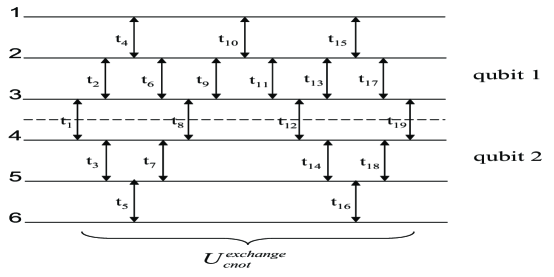
Figure 1: Circuit diagram for implementing a CNOT gate between logical qubits 1 and 2. Logical qubit 1 is encoded in the top three physical qubits, 1-3, and logical qubit 2 in the bottom three physical qubits, 4-6. Each vertical line connecting two physical qubits represents an exchange gate with strength $J_{0}$ switched on for time $t_{s}$. As a result of the symmetry of the gate sequence, only 7 independent variables are required to define the gate times of the entire 19-gate sequence.⁽DiVincenzo et al. (2000)⁾

It should be noted that 19 is an upper limit on the number of serial exchanges required, obtained through numerical optimization of the Makhlin invariants⁽Makhlin (2002)⁾, and it is possible that a smaller number might suffice. The number of exchange operations can also be reduced if one considers a more complex quantum dot architecture that supports non-nearest neighbour interactions, rather than the linear array studied here. In particular, if in addition to exchanges $H_{ii+1}$, any $H_{ij}$ connection is accessible, then full parallelism is possible. With parallel exchanges of this type a one-qubit rotation can be shown to require only 3 exchanges, and a CNOT gate only 8 exchanges.⁽DiVincenzo et al. (2000)⁾

Universal quantum information processing will require that we can implement the CNOT gate between any two logical qubits, and not just between adjacent qubits. This need is apparent even for such simple algorithms as the three qubit Deutsch-Josza algorithm that tests whether an arbitrary function is balanced or constant.⁽Nielsen and Chuang (2000)⁾ We shall see below that one of the black box gate sequences describing a balanced function for the three qubit Deutsch-Josza algorithm requires a CNOT gate between qubits 1 and 3. We shall refer to this as CNOT(1,3). Analysis of truth tables for combinations of CNOTs between neighbouring dots readily shows that a CNOT(1,3) gate is equivalent to a pairwise sequence of four CNOT gates between adjacent dots, as illustrated in Fig. 2

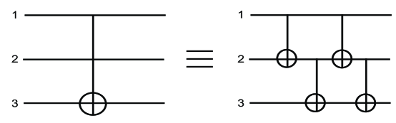
Figure 2: Equivalence of circuit employing only CNOT gates between adjacent logical qubits, to a circuit representing a CNOT between qubits 1 and 3.

It would be perfectly valid to employ this pairwise adjacent sequence to represent CNOT(1,3). However, since each CNOT requires 19 exchange operations, this would entail implementing a total of $4*19=76$ exchange gates. Here, recognition of the relation between exchange and SWAP operations allows for a more efficient solution. We note that any exchange gate when applied for a duration equivalent to a $\pi$ pulse, yields the SWAP operation, and that exchange gates may be inter converted by action of the appropriate SWAP operations, e.g.,

$$\exp{(itH_{13}/\hbar)}=\exp{(i\pi H_{23}/\hbar)}\exp{(itH_{12}/\hbar)}\exp{(i\pi H_{23}/\hbar)}.$$ (4)

Combining an exchange gate between logical qubits $i$ and $i+1$ with exchange-generated SWAP operations immediately before and after, thereby makes the exchange operational between any two qubits $i$ and $j$. This is summarized by the following:

$$\exp{(itH_{ij}/\hbar)}=\prod_{k=i+1}^{j-1}\exp{\left(i\pi H_{kk+1}/\hbar\right)}\exp{\left(itH_{ii+1}/\hbar\right)}\prod_{k=j-1}^{i+1}\exp{\left(i\pi H_{kk+1}/\hbar\right)}.$$ (5)

Making use of this relation, we find that a CNOT gate between qubits 1 and 3 can now be performed with only 55 exchanges, an overall saving of 21 operations compared with the pairwise adjacent scenario depicted in Fig 2.

II.1 The exact CNOT

The Makhlin invariants⁽Makhlin (2002)⁾ guarantee a sequence of exchange gates and times that provide a two-qubit unitary $U_{cnot}^{exchange}$ which is locally equivalent to the CNOT. This is not necessarily equal to CNOT in the computational basis. To use our exchange-only CNOT in conjunction with other gates, we therefore need to find a set of local unitaries that transform this locally equivalent gate to the CNOT in the computational basis. Mathematically, we can represent the transformation as:

$$CNOT\,=\,\left(U_{1}\otimes U_{2}\right)\,U_{cnot}^{exchange}\\ \,\left(V_{1}\otimes V_{2}\right).$$ (6)

Here $U_{1}$, $U_{2}$, $V_{1}$, and $V_{2}$ designate local basis transformations each consisting of at most 4 exchange gates⁽DiVincenzo et al. (2000)⁾ that act on the first or the second logical qubit. For $U_{cnot}^{exchange}$ we employ here the optimized sequence of 19 exchange gates from Ref. DiVincenzo et al., 2000. It is then possible, using a procedure introduced by Makhlin⁽Makhlin (2002)⁾, to find the local unitaries ($U_{1}$, $U_{2}$, $V_{1}$, and $V_{2}$) by i) recasting $U_{cnot}^{exchange}$ in the Bell basis, $M_{B}=Q^{\dagger}U_{cnot}^{exchange}Q$, ii) evaluating the spectrum of $m=M_{B}^{T}M_{B}$, and iii) then relating this matrix of eigenvalues to the corresponding matrix for the CNOT gate in the computational basis. Here $Q$ is the matrix that transforms $U_{cnot}^{exchange}$ from the computational basis to the Bell basis, and $M_{B}^{T}$ is the matrix transpose of $M_{B}$. Having obtained the local unitaries $U_{i}$ and $V_{i}$, $i=1,2$, it remains to decompose these into an actual sequence of exchange gates in order to perform full exchange-only computation. We describe here two ways to accomplish this decomposition. The first is a general procedure based on numerical optimization. The second is an analytic procedure that is specific to the present case, since it relies on the ability to find analytic solutions to systems of trigonometric equations that may be less tractable for other situations.

For both approaches we give the times $t_{s}$ for the individual exchange gates in units of $2\hbar/J_{0}$. We cite all time values as positive numbers here, and implicitly assume that the pulse-integrated exchange coupling value $J_{0}$ is constant. (In Ref. Burkard et al., 1999, Burkard et al. consider the possibility of tuning the Heisenberg interaction around the point of zero coupling, thus allowing $J_{0}$ to assume both positive and negative values.) Note that all gate times are defined modulo $\pi$, i.e. an exchange gate implemented for $t_{s}$ is identical (up to a global phase of -1) to one implemented for $t_{s}+\pi$ (see discussion above and Refs. Loss and DiVincenzo, 1998 and DiVincenzo et al., 2000).

For the numerical optimization procedure, we first express the local basis transformations, $U_{1}$, $U_{2}$, $V_{1}$, and $V_{2}$, as sequences of 4 exchange gates. We then use a version of the Nelder-Mead simplex algorithm⁽Nelder and Mead (1965)⁾ to find those sequences that minimize both the matrix distance from the resulting CNOT gate Eq. (6) to the true CNOT in the computational basis, and the extent of leakage out of the encoded subspace. The Nelder-Mead algorithm is an example of a direct search method, i.e. it uses only function evaluations and does not rely upon any derivative information about the cost function. Each iteration begins with a geometric figure, a simplex, created from $m+1$ coordinates in parameter space, where $m$ is the number of variables of the cost function to be optimized. From this first simplex, new points are generated and the cost function is evaluated at these new coordinates. A new simplex, possessing better descent characteristics than the previous, is then generated from the cost function evaluations and the new test points.⁽Lagarias et al. (1995)⁾ The Nelder-Mead method is known to work well in low-dimensional instances such as those studied here. The local character of the method is nevertheless a concern. To avoid getting trapped in local minima, the parameter space must be densely sampled. We accomplish this here by shooting initial coordinates into parameter space, followed by optimization from the coordinate that gave the smallest initial value of the cost function.

As noted above, our cost function contains two components. First, it includes an element by element matrix equivalence criteria, i.e. the matrix distance between the target gate (the true CNOT) and the candidate exchange-only representation of this, Eq. (6), which is constructed from the 19-exchange sequence of Ref. DiVincenzo et al., 2000 together with two 8-exchange sequences representing the local unitaries. Second, it contains a component that provides a penalty for leakage out of the encoded subspace, namely the sum of the absolute value of all matrix elements connecting states in the encoded logical subspace to states outside this subspace, illustrated in Fig. 3.

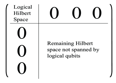
Figure 3: To ensure that our encoded unitary does not leak, we require that the encoded unitary, $\left(U_{1}\otimes U_{2}\right)\,U_{cnot}^{exchange}\,\left(V_{1}\otimes V_{2}\right)$, can be represented by the above matrix decomposition. The logical Hilbert space has dimension $2^{n}\times 2^{n}$ for n logical qubits. The complete Hilbert space has dimension $2^{N}\times 2^{N}$, corresponding to N physical qubits.

These two requirements of minimal matrix distance from the target CNOT and non-leakage from the encoded subspace lead to the following expression for the cost function:

$$C=\sum_{i,j}^{2^{n}}|U_{cnot}^{exchange}(i,j)-CNOT(i,j)|+\ \sum_{2^{n}<i<2^{N}\atop j\leq 2^{n}}\ |U_{cnot}^{exchange}(i,j)|,$$ (7)

where $n$ is the number of logical qubits and $N$ the number of physical qubits. The first summation represents the matrix distance between Eq. (6) and the target CNOT, and the second summation, which goes over the lower left-hand block of the matrix in Fig. 3, represents the extent of leakage. The second summation thus consists of terms connecting basis states $j\leq 2^{n}$ inside the encoded logical subspace to all basis states $2^{n}<i\leq 2^{N}$ outside the encoded logical subspace.

Since we employ the 19-exchange sequence for $U_{cnot}^{exchange}$ from Ref. DiVincenzo et al., 2000, the numerical optimization is restricted here to the two sets of 8-exchange sequences representing $U_{1}\otimes U_{2}$ and $V_{1}\otimes V_{2}$, respectively. We implement this by constructing a sequence of 35 gates (i.e., 4+4+19+4+4, see Fig. 4) with gates 9-27 taken from Ref. DiVincenzo et al., 2000, and then optimizing the cost function $C$, Eq. (7), for the matrix resulting from the entire 35-exchange sequence only over the 16-dimensional parameter space of the two 8-exchange sequences. We note that since the available nearest neighbor exchanges $E_{12}$ and $E_{23}$ correspond simply to rotations of the logical states around the z-axis and about an axis oriented along $\sqrt{3}/2\sigma_{x}+1/2\sigma_{z}$, respectively⁽Kempe et al. (2001); DiVincenzo et al. (2000)⁾, the exchange-based local gates will therefore not take states outside the logical subspace and will hence not add to the leakage term. The leakage parameter is therefore determined solely by the accuracy of the underlying gate sequence for $U_{cnot}^{exchange}$.

We have found that for such a 35-gate sequence, the overall cost function C can readily be reduced to less than $10^{-4}$ by this numerical optimization. More specifically, we find that the matrix distance (first term of Eq. 7) between this 35 gate long sequence and the exact CNOT is $1\times 10^{-5}$ and that the leakage term (second term of Eq. 7) is $5\times 10^{-9}$ (equal to the value for $U_{cnot}^{exchange}$, as noted above). This level of optimization corresponds to a maximum element matrix distance from CNOT (i.e., maximum matrix element inaccuracy) of $5\times 10^{-6}$. The optimal exchange-only sequences for the local transformations are summarized in Fig. 4 and in Table 1, respectively.

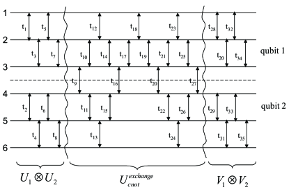
Figure 4: Diagrammatic representation of one set of exchange gates that transform the 19-exchange gate CNOT ($U_{cnot}^{exchange}$) into the exact CNOT. These 8+8 gate times ($t_{1}$-$t_{8}$ and $t_{28}$-$t_{35}$) were arrived at numerically using the Nelder-Mead simplex method⁽Nelder and Mead (1965)⁾ as described in the text. The corresponding 35 gate times given in Table 1 will generate the exact CNOT to within a cost function value $C=10^{-5}$, corresponding to a maximum matrix element distance of $5\times 10^{-6}$.

The second approach to finding an exchange-only representation of the local unitaries is analytic solution through matrix manipulations, as follows. We first analyze the similarity transformation $S$ that diagonalizes $U_{cnot}^{exch}$ from Ref. DiVincenzo et al., 2000 in the computational basis, i.e., $S^{\dagger}U_{cnot}^{exchange}S=D$ where $D$ is a diagonal 4-by-4 matrix. We found that $S$ can be expressed as local operations on the logical qubits, namely $S=I\otimes\left(\frac{\sqrt{3}}{2}I-\frac{i}{2}\sigma_{y}\right)$. Mapping the $SU(2)$ spin rotations to rotations in $SO(3)$ and using the quaternion representation for $SO(3)$ rotations (see Appendix A for details), we find that this similarity transformation can be realized using only 3 exchange gates. From the diagonal matrix $D$, one can then readily generate a C-PHASE gate in the computational basis by merely performing rotations around the z-axis. Transformation of the resulting C-PHASE into the desired CNOT is subsequently realized by acting with Hadamard gates on the second logical qubit both before and after the resulting C-PHASE. These elementary gates are summarized in Fig. 5. Both the $\sigma_{z}$ rotations and the Hadamard gate have analytic exchange-only solutions on the encoded subspace (see Sec. II.2 and Fig. 7). We thereby arrive at an alternative, fully analytic solution for an exchange-only realization of the local unitary transformations into the computational basis, requiring a total of 33 exchange gates. These may be reduced to a total of 30 exchanges by combining the times of any sequential exchanges on the same pairs of qubits that occur as a result of juxtaposition of elementary gates. Consequently the desired overall transformation can now be completed with only 11 more exchanges than the underlying 19-exchange sequence for $U_{cnot}^{exchange}$. Fig. 6 and Table 2 summarize the resulting gate sequence and gate times, respectively, for the exact CNOT deriving from this analytic solution of the local transformations.

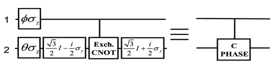
(a) A single qubit gate ($\frac{\sqrt{3}}{2}-\frac{i}{2}\sigma_{y}$) acting on the second logical qubit diagonalizes the 19-gate exchange sequence. The resulting diagonal 4-by-4 matrix is then converted into the C-PHASE by $\sigma_{z}$-rotations acting on both the first and the second qubit, with angles $\phi=0.612497$ and $\theta=-0.547580$, respectively. These values are determined from the analytic solutions to a linear equation system with 3 unknowns: $\phi$, $\theta$ and a global phase. See Appendix A for details as to how these parameters were obtained.

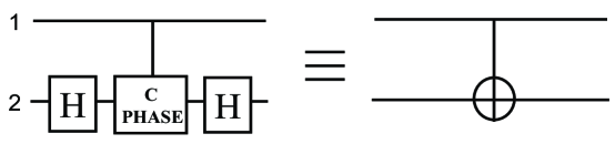
(b) The C-PHASE gate can be transformed into the CNOT gate by acting with Hadamard gates on the second qubit before and after the C-PHASE gate.

Figure 5: Representation of analytic sequence of local transformations that transform the 19-exchange sequence $U_{cnot}^{exchange}$ from Ref. DiVincenzo et al., 2000 into the true CNOT in the computational basis. The exchange gates and times corresponding to the elementary local transformations are then obtained using the quaternion representation of the desired $SU(2)$ unitaries (see Appendix A for details).

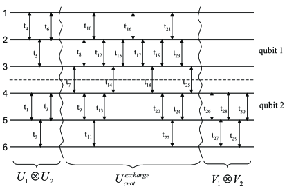
Figure 6: Diagrammatic representation of a second, shorter set of 30 exchanges that transform the 19 exchange-only CNOT into the exact CNOT in the computational basis. Here $U_{cnot}^{exchange}$ corresponds to the 19 gate sequence of Ref. DiVincenzo et al., 2000. The remaining gates and gate times, $t_{1}$-$t_{6}$ and $t_{26}$-$t_{30}$, correspond to the local unitaries ($U_{1}$, $U_{2}$, $V_{1}$, and $V_{2}$) which were arrived at analytically by decomposing the local unitaries into a sequence of elementary rotations in $SU(2)$ as summarized in Fig. 5, and then using the quaternion representation of the corresponding rotations in $SO(3)$ to find the sequences of exchange gates and the times, $t_{s}$, that generate them (Appendix A). The resulting gate times are listed in Table 2.

The analytical sequence of Table 2 result in a maximum matrix element deviation of $5.5\times 10^{-6}$ from the true CNOT. Thus, our analytic solution has similar accuracy as the numerical solution above. However, the 30-exchange analytical sequence in Fig. 6 and Table 2 represents a saving in both total number of gates and total time, relative to the 35-exchange sequence of Fig. 4 and Table 1). The 30-exchange sequence requires total time $T_{30}=43.373$, compared with $T_{35}=54.326$ for the 35-exchange sequence. This is an advantage for experimental implementation, since the shorter time allows for less decoherence.

II.2 Single Qubit Gates through Exchange

By considering the action of the Heisenberg Hamiltonian on the encoded subspace, Eq. 3, it was found numerically in Ref. DiVincenzo et al., 2000 that arbitrary single-qubit gates can be performed on the 3-qubit encoding using 4 nearest neighbour exchanges in serial operation mode, or by using 3 exchanges in parallel.

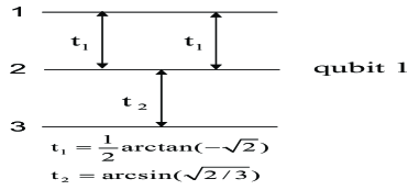
(a) The Hadamard gate can be implemented with 3 exchange gates.

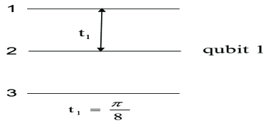
(b) The T gate (T=$\pi/8$ rotation about $\hat{z}$) can be implemented with just one exchange gate since $E_{12}=-\sigma_{z}$, where $\sigma_{z}$ refers to a z-rotation in the encoded logical subspace.

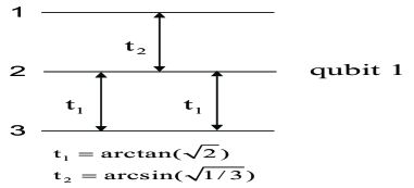
(c) The NOT gate can also be implemented with 3 exchange gates

Figure 7: Exchange-only representation of encoded single qubit gates can often be arrived at from geometric considerations. The exchange-only representations of the Hadamard gate, the $\pi/8$, and the NOT gate given here were obtained using a quaternion representation for the corresponding rotations in $SO(3)$ (Appendix A).

The exchange gate times $t_{s}$ for a particular single-qubit gate can in principle be found by solving a system of equations with four unknowns. Specifically, given a single-qubit gate $A$, we consider the sequence of 4 exchange gates

$$A=\exp{(-it_{4}E_{12}/\hbar)}\exp{(-it_{3}E_{23}/\hbar)}\ \exp{(-it_{2}E_{12}/\hbar)}\exp{(-it_{1}E_{23}/\hbar)}$$ (8)

and solve the 4 coupled equations for the 4 times $t_{s}$, $s=1\,-\,4$:

$$A_{00} = \exp{(i(t_{2}+t_{4}))}\left(cos(t_{3})-\frac{i}{2}sin(t_{3})\right)\ \left(cos(t_{1})-\frac{i}{2}sin(t_{1})\right)$$

$$-\frac{3}{4}\exp{(i(t_{4}-t_{2}))}sin(t_{1})sin(t_{3})$$

$$A_{01} = -i\frac{\sqrt{3}}{2}\exp{(i(t_{2}+t_{4}))}sin(t_{1})\ \left(cos(t_{3})-\frac{i}{2}sin(t_{3})\right)$$

$$-i\frac{\sqrt{3}}{2}\exp{(i(t_{4}-t_{2}))}sin(t_{3})\ \left(cos(t_{1})+\frac{i}{2}sin(t_{1})\right)$$

$$A_{10} = -i\frac{\sqrt{3}}{2}\exp{(i(t_{2}-t_{4}))}sin(t_{3})\ \left(cos(t_{1})-\frac{i}{2}sin(t_{1})\right)$$

$$-i\frac{\sqrt{3}}{2}\exp{(-i(t_{4}+t_{2}))}sin(t_{1})\ \left(cos(t_{3})+\frac{i}{2}sin(t_{3})\right)$$

$$A_{11} = -\frac{3}{4}\exp{(-i(t_{2}-t_{4}))}sin(t_{1})sin(t_{3})$$ (9)

$$+\exp{(-i(t_{2}+t_{4}))}\left(cos(t_{3})+\frac{i}{2}\ sin(t_{3})\right)\left(cos(t_{1})+\frac{i}{2}sin(t_{1})\right).$$

Here we have used the properties of the exchange operators $E_{12}=-\sigma_{z}$ and $E_{23}=\sqrt{3}/2\sigma_{x}+1/2\sigma_{z}$ in the logical basis⁽Kempe et al. (2001); DiVincenzo et al. (2000)⁾.

In this work we used a quaternion approach to represent the single qubit gates as rotations in $SO(3)$, rather than solving the above coupled equations. Obtaining the exchange gate times in the quaternion representation also requires solving trigonometric equations in multiple unknowns, but these equations, especially for simpler gates, are often more straightforward than the matrix equation above, and analytic solutions easier to obtain. We first recognize that the combinations of the two exchanges $E_{12}$ and $E_{23}$ generate the encoded single qubit operations $\sigma_{z}$ and $\sigma_{x}$, and thereby will suffice to generate any arbitrary rotation on $SU(2)$. A single qubit gate is then mapped from $SU(2)$ to $SO(3)$⁽Sakurai (1994)⁾ where the desired rotation can be decomposed as a sequence of quaternions. The quaternion approach is convenient for finding an analytic solution for realization with a given number of exchanges, as described in Appendix A.

Using this approach we found exchange-only gate sequences for the $\pi/8$ gate (the T gate⁽Nielsen and Chuang (2000)⁾), the NOT gate, and the Hadamard gate. A full description of these solutions is given in Appendix A. We found that both the Hadamard and the NOT gate can be obtained from a sequence of three exchange gates, while the $\pi/8$ gate requires only one exchange gate. The corresponding gate sequences and gate times are shown in Fig. 7. (Note that any $\sigma_{z}$ rotation by $\theta$ ($R_{z}(\theta)=exp(-i\theta\sigma_{z})$) can be realized as $exp(i\theta E_{12})$).

A third approach to finding the exchange-only implementation of the single qubit gates is through a Nelder-Mead simplex numerical optimization⁽Nelder and Mead (1965); Lagarias et al. (1995)⁾, as implemented for the local transformations in the previous section. Though not analytic, the Nelder-Mead approach is often much faster than analytic solutions and for single qubit gates the cost function can readily be reduced to zero at the machine precision level.

III Deutsch-Josza Algorithm and Algorithmic Fidelity

There are currently several quantum algorithms that show speed-up over their classical analogs.⁽Nielsen and Chuang (2000)⁾ Any one of these algorithms serve to investigate the merits of the exchange-coupled quantum dot implementation.

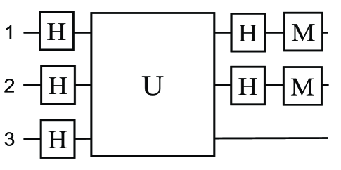
Figure 8: A circuit digram depiction of the Deutsch-Josza algorithm for three qubits. The two top most qubits are the query qubits and make up the domain for the unknown function $f:\{0,1\}^{n}\mapsto\{0,1\}$⁽Nielsen and Chuang (2000)⁾, here indicated by $U$ a unitary spanning all three qubits. For the three qubit Deutsch-Josza there are eight possible U’s, all of which are given in Fig. 9. Evaluation of $U$ is preceded and followed by Hadamard gates $[H]$. The result of the function evaluation is stored in the answer qubit, the bottom-most qubit in the circuit diagram, as $y\,=\,|y\;\oplus f(x_{1},x_{2})\,\rangle$, where $x_{1}$ and $x_{2}$ designate the bit values of query qubit 1 and 2 respectively. The outcome of the measurement of the query qubits, here designated by M, answers whether the function is constant or balanced.

We have chosen the Deutsch-Josza algorithm, a relatively simple algorithm requiring only a few logical gates (Fig. 8).

The objective of the Deutsch-Josza algorithm is to determine if an unknown function, $f:\{0,1\}^{n}\mapsto\{0,1\}$, is balanced (i.e. equal number of zeros and ones) or constant. For the three qubit Deutsch-Josza with its two query qubits and one answer qubit, this corresponds to 8 possible functions, six balanced functions and two constant functions. In Fig.  9 these functions are expressed in circuit diagram form.

The existence of 8 different functions, and consequently of eight different versions of the algorithm, implies different fidelity values for a given initial state, $\rho_{0}(0)=\rho(0)$, for each version. For each version of the algorithm and for each choice of dephasing rate, we evaluate the fidelity according to

$$F=Tr\{\rho_{0}(t_{f})\rho(t_{f})\},$$ (10)

where $\rho_{0}(t_{f})$ is the density matrix describing system evolution in the absence of errors, and $\rho(t_{f})$ the density matrix describing evolution in the presence of errors.

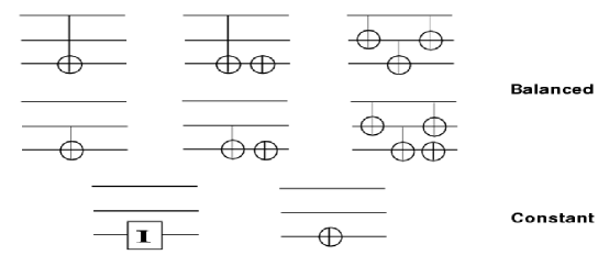
Figure 9: Circuit diagram representation of the eight different black box function evaluations (the U’s of Fig. 8) inherent in the three qubit Deutsch-Josza algorithm. For 3 qubits the algorithm results in six balanced and two constant functions.

Both $\rho_{0}(t_{f})$ and $\rho(t_{f})$ are evaluated over the time $t_{f}$ required to complete that version of the algorithm. We define the algorithmic fidelity to be the worst-case fidelity, namely, for a given value of the dephasing rate, the fidelity of that version of the algorithm having the lowest fidelity. This provides a more conservative estimate than averaging over the 8 different fidelities resulting from each version of the algorithm.

IV Numerical Methods

As discussed in section II, universal computation with the exchange interaction requires at least three physical qubits for every encoded logical qubit.⁽Kempe et al. (2001)⁾ Thus, the Hilbert space grows as $8^{n}$, where $n$ is the number of logical qubits, and simulation of the density matrix becomes time consuming even for a few logical qubits. To permit consideration of larger numbers of logical qubits we use here the Monte Carlo wave function method.⁽Dalibard et al. (1992)⁾ This approach scales linearly with the size of the Hilbert space rather than quadratically as master equation methods.

IV.1 Monte Carlo Wave-functions

The Monte Carlo wave function approach, also known as the method of Quantum Trajectories or the “Quantum Jump” approach, was originally developed within the quantum optics community.⁽Dalibard et al. (1992); Mølmer et al. (1993); Hegerfeldt and Wilser (1991)⁾ The method relies on a twofold approach to the system evolution. First, an effective Hamiltonian gives rise to a continuous non-unitary evolution of the system wave function. Second, decay operators, identical to the Lindblad operators within the master equation formalism⁽Carmichael (1993)⁾, give rise to stochastic discontinuities in the wave function. These stochastic discontinuities resemble the jumps one might expect from a single isolated quantum system.

Both the effective Hamiltonian and the decay terms can be obtained from the Lindblad master equation.⁽Carmichael (1993)⁾ The conditional, or effective, Hamiltonian is given by

$$H_{cond}=H_{sys}-\frac{i\hbar}{2}\sum_{m}C_{m}^{{\dagger}}C_{m},$$ (11)

where $H_{sys}$ is the system Hamiltonian and the $C_{m}$’s are decay terms resulting from the system-environment interaction with a subsequent tracing over the bath degrees of freedom. The total time evolution under $H_{cond}$ is discretized and at each time step the probability of any collapse event is calculated:

$$P_{tot}=\sum_{m}\delta P_{m}=\sum_{m}\Delta t\ \langle\Psi(t)|C_{m}^{{\dagger}}C_{m}|\Psi(t)\rangle.$$ (12)

This total collapse probability accounts for the occurrence of any error event, $C_{m}^{{\dagger}}C_{m}$, that collapses the system wave-function. The calculated $P_{tot}$ is compared against a random number, $r$, taken from a uniform distribution. This is the first Monte Carlo test. A random number less than the total collapse probability, $r<P_{tot}$, designates that an error has occurred. Another Monte Carlo test, involving another random number, decides which error occurs. This second random number, $s$, is compared against the normalized collapse probabilities, $\delta P_{m}/P_{tot}$, and that error is chosen that first makes the sum of the normalized error probabilities greater than the random number. Thus, upon completion of the two Monte Carlo tests the new wave-function is:

$$|\Psi(t+\Delta t)\rangle=\frac{C_{i}|\Psi(t)\rangle}{|\langle\Psi(t)|C_{m}^{{\dagger}}C_{m}|\Psi(t)\rangle|^{1/2}},$$ (13)

where $C_{i}$ is the error operator randomly chosen in the second Monte Carlo test such that $\sum_{m=1}^{i}\delta P_{m}/P_{tot}>s$.

On the other hand, if $r$ is greater than $P_{tot}$, the system state is propagated according to $H_{cond}$ and we obtain the system state at $t+\Delta t$:

$$|\Psi(t+\Delta t)\rangle^{\prime}=\exp{\left(-i\Delta tH_{cond}/\hbar\right)}|\Psi(t)\rangle.$$ (14)

Since $H_{cond}$ is non-Hermitian the norm decreases over time. To ensure equivalence with other approaches to simulating open quantum systems, e.g. master equations⁽Carmichael (1993)⁾, the wave-function must be renormalized at the end of every time step:

$$|\Psi(t+\Delta t)\rangle=\frac{|\Psi(t+\Delta t)\rangle^{\prime}}{|\langle\Psi(t+\Delta t)|^{\prime}|\Psi(t+\Delta t)\rangle^{\prime}|^{1/2}}.$$ (15)

Upon renormalization a new total collapse probability is calculated and the entire algorithm begins anew for the next timestep.

The time step, $\Delta t$, must be chosen such that $P_{tot}\ll 1$, since for too large time steps a perturbative expansion for calculating the error probabilities is no longer justified. Each trajectory corresponds to a possible evolution of a single quantum system. The fidelity measure is based on the density matrix which can be regained by averaging over many trajectories.⁽Mølmer et al. (1993)⁾ Use of Eq.( 10) leads to the following expression for the fidelity:

$$F=\frac{1}{N_{traj}}\sum_{n=1}^{N_{traj}}\mid\langle\Psi_{0}(t_{f})||\Psi_{n}(t_{f})\rangle\mid^{2}.$$ (16)

Here $|\Psi_{n}(t_{f})\rangle$ is the wavefunction for trajectory $n$ propagated with decoherence, and $|\Psi_{0}(t_{f})\rangle$ is the wavefunction propagated in the absence of decoherence. Simulations are run with increasing numbers of trajectories until the fidelity converges. To ensure that the fidelity we obtain contains no artifacts or anomalies due to the choice of the initial system state, we sample a random distribution of initial states, all located on the surface of the hyperdimensional Bloch sphere of logical basis states. These Bloch states are given by:

$$|\Psi(t)\rangle= \sum_{i=0}^{N-1}c_{i}(t)|\psi\rangle$$

$$c_{k}(0)= \exp{(i\varphi_{k})}\prod_{i=0}^{N-k} \cos{\theta}_{i}\ \prod_{j=N-k}^{N-1}\sin{\theta}_{j}$$

$$\varphi_{0}=0, \theta_{0}=\pi.$$ (17)

IV.2 Split Operator Method

The dimensionality of the CNOT gate simulation on 6 physical qubits, a $2^{6}=64$ dimensional Hilbert space, is still small enough to permit the use of an exact diagonalization method to construct the conditional time evolution operator from $H_{cond}$. However, the three qubit Deutsch-Josza algorithm requires nine physical qubits within the exchange-only model, and $H_{cond}$ must then be exponentiated on a $2^{9}=512$ dimensional space. We have developed a more efficient method to construct $U_{cond}=exp(-iH_{cond}t/\hbar)$, that proves computationally efficient for even larger Hilbert spaces. We make use of a split-operator decomposition of $U_{cond}$ that is based upon the fact that $H_{cond}$, including decay elements, can be split up into a term diagonal in the spin components and a term off-diagonal in the spin components. The diagonal part can be expressed as

$$D=J\,S_{i,z}\cdot S_{j,z}-2i\hbar\Gamma_{dep}\sum_{i=1}^{N}S_{z,i}^{\dagger}S_{z,i},$$ (18)

and the off-diagonal part as

$$T=\frac{J}{2}(S^{+}_{i}S^{-}_{j}+S^{+}_{i}S^{-}_{j})-2i\hbar\Gamma_{emi}\sum_{i=1}^{N}S^{+}_{i}S^{-}_{i}.$$ (19)

Here $\Gamma_{dep}$ and $\Gamma_{emi}$ are the single spin pure dephasing and emission rates obtained from theoretical and experimental estimates and measurements Awschalom and Kikkawa (1999); Gupta et al. (1999); Kikkawa et al. (1997); Fujisawa et al. (2001).

The time evolution operator, $U_{cond}$, can then be expanded in an approximation accurate up to second order in $\Delta t$ (errors  $O(\Delta t^{3})$) as:

$$U_{cond}\approx\exp{\left(-iD\Delta t/2\hbar\right)}\ \exp{\left(-iT\Delta t/\hbar\right)}\ \exp{\left(-iD\Delta t/2\hbar\right)}.$$ (20)

The simulation of $U_{cond}(t)$ now reduces to consecutive application of the exponentiated operators D and T. This can be efficiently done if states are represented by integers in binary notation, i.e. each spin is represented in the $S_{z}$ basis by a 0 or a 1 at location j in the binary representation of the state vector $x=|k_{1}...k_{N}\rangle$. The spin operators can be recast as binary shift and logic operations

$$S_{z}|k_{1}k_{2}...k_{j}...k_{N}\rangle = \frac{1}{2}(1-2*ibits(k,j,1))\,|k_{1}k_{2}...k_{j}...k_{N}\rangle,$$ (21)

$$S^{+}|k_{1}k_{2}...k_{j}...k_{N}\rangle = (1-ibits(k,j,1))|k_{1}k_{2}...ibits(k,j,1)+1...k_{N}\rangle,$$ (22)

$$S^{-}|k_{1}k_{2}...k_{j}...k_{N}\rangle = ibits(k,j,1)|k_{1}k_{2}...ibits(k,j,1)-1...k_{N}\rangle,$$ (23)

where ibits denotes a compiler (F90) command that extracts the value of jth bit in integer k. These binary operations are seen to act upon the system state vector in a manner analogous to raising and lowering operators. With this approach it becomes possible to simulate very large Hilbert spaces. This approach was employed previously in a checkerboard time propagation scheme for study of many body dynamics of interacting particles on lattices.⁽Zhang and Whaley (1991, 1992)⁾

IV.3 Parameters

Data with regards to decoherence parameters for exchange coupled quantum dots is scarce. We have used experimental parameters to the extent possible. Where none are available we have interpolated, using theoretical estimates, between what is experimentally known and the requirements of our simulations. In general, experiments in condensed matter physics have indicated that the electron spin states, because of their weaker coupling to the environment, exhibit longer coherence times than the charge states. Due to difficulties involved in measuring single spin states, however, the majority of these experiments provide us with a ensemble measurement of the lifetime, and are thus not directly applicable to a system of single spins⁽Awschalom and Kikkawa (1999); Gupta et al. (1999); Kikkawa et al. (1997)⁾ We employ here the inequality relationship $T_{1}\geq T_{2}\geq T_{2}^{*}$, where $T_{1}$ describes the time scale for the spins’ exchange of energy with the surrounding matrix, $T_{2}$ is the single spin decoherence time, and $T_{2}^{*}$ is an ensemble decoherence time which, in addition to contributions from $T_{1}$ and $T_{2}$, also contains effects due to inhomogeneities in the system, to the surrounding matrix, and to the control fields.⁽Engel and Loss (2001)⁾ Taking into account the single dot $T_{1}$ times obtained by Fujisawawa et al.⁽Fujisawa et al. (2001)⁾, we arrive at a set of reasonable decoherence parameters: a dephasing rate on the order of ns and a timescale of $\mu$s for emission and absorption, both of which involve spin flips. Consequently, in a system like ours, where the strength of the exchange coupling is assumed to be on the order of 0.2 $meV$, we find dimensionless decoherence rates $\hbar\Gamma/J_{0}\,=\,10^{-3}\,-\,10^{-5}$. Additionally, we find that dephasing errors dominate over emission events, according to $\frac{\Gamma_{dep}}{\Gamma_{emi}}=\frac{1/T_{2}}{1/T_{1}}\simeq 10^{2}$. Consequently, pure dephasing is a greater concern than spin flip errors, and will thus constitute the main focus of our simulations. In the context of decoherence, it should be noted that a reduction of some of the decoherence pathways may be possible with the use of experimental techniques such as spin polarization and spin echo, that have been developed for other systems such as NMR.⁽Hahn (1950)⁾ Our simulation does not include these potentially very beneficial modifications. Note that the encoding in Eq. (3) is automatically protected against collective dephasing, but not against independent single spin dephasing.

V Results

V.1 Exchange-only CNOT, in serial mode

The encoded exchange-only CNOT is the first unitary operation we investigate. Fig. 10 shows the fidelity over the 19 gate implementation. We see that for a dimensionless dephasing rate of $\hbar\Gamma\,/\,J_{0}\,=\,10^{-3}$ the probability of perfectly performing a CNOT is $\sim 98\%$.

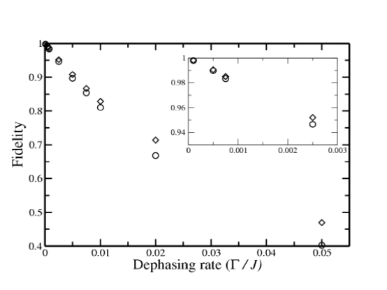
Figure 10: Fidelity simulation for CNOT gate, subject to dephasing errors, for a linear quantum dot array, where three physical qubits encodes each logical qubit. $\circ$ 19 exchange gate implementation of CNOT gate. $\diamond$ Free system evolution for duration equivalent to CNOT.

Burkard et al. have indicated a possibility that actual implementation of the gate, i.e. turning on the $J_{0}$ coupling between adjacent quantum dots, might result in faster decoherence.⁽Burkard et al. (1999)⁾ We therefore used the free system evolution under identical conditions of dephasing as a point of reference. We find that gate implementation does result in faster decoherence, but that the effects only become appreciable at higher dephasing rates, $\hbar\Gamma_{dep}/J_{0}=10^{-2}$ (Fig. 10). We also compared the fidelity obtained for the encoded CNOT gate to a standard CNOT gate between two physical qubits. To reduce the effects of method and parameter choice, we used the same values for the dephasing rate to interdot coupling strength ratio, $\hbar\Gamma_{dep}/J_{0}$, and took the timescale for the CNOT gate to be the same as for the exchange coupled qubits. This comparison is shown in Fig. 11.

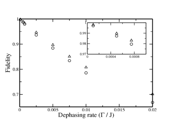
Figure 11: Fidelity simulation for a CNOT gate, subject to dephasing errors, for an encoded linear quantum dot array and between two physical qubits. $\circ$ 19 exchange gate implementation of CNOT gate. $\bigtriangleup$ CNOT gate implemented between two physical qubits, with gate time equal to 19 exchange gates.

Fig. 11 shows that the performance of the encoded CNOT gate deteriorates faster with increasing dephasing rates than does the bare CNOT gate. We recall that the timescale for coherence loss due to dephasing decreases with the number of qubits. As shown in Ref. Carmichael, 1993 the master equation for a single qubit under pure dephasing can be written as:

$$\dot{\rho}(t)=-\frac{i\omega}{2}[\sigma_{z},\rho(t)]+\frac{\Gamma_{dep}}{2}(\sigma_{z}\rho(t)\sigma_{z}-\rho(t)),$$ (24)

where $\omega$ is the shifted frequency of the two level system and $\Gamma_{dep}$ is the dephasing rate. The dynamics of Eq. (24 can be solved analytically and for this 2-level system the fidelity (see Eq. (10)) is obtained as:

$$F = Tr\,\left\{\left(\begin{array}[]{cc}\rho_{00}(0)&\rho_{01}(0)e^{-iwt}\\ \rho_{10}(0)e^{iwt}&\rho_{11}(0)\end{array}\right)\left(\begin{array}[]{cc}\rho_{00}(0)&\rho_{01}(0)e^{-iwt-\Gamma_{dep}t}\\ \rho_{10}(0)e^{iwt-\Gamma_{dep}t}&\rho_{11}(0)\end{array}\right)\right\}$$ (29)

$$= \rho_{00}^{2}(0)+\rho_{11}^{2}(0)+e^{-\Gamma_{dep}t}(|\rho_{01}(0)|^{2}+|\rho_{10}(0)|^{2})$$ (30)

This state-dependent fidelity must now be integrated over all possible initial states to obtain the algorithmic fidelity. Employing a general state $\Psi(0)=\cos{\frac{\theta}{2}}|0\rangle+e^{i\phi}\sin{\frac{\theta}{2}}|1\rangle$ and integrating over all possible states on the surface of the Bloch sphere leads to the average fidelity:

$$\bar{F}(t) = \frac{1}{4\pi}\int_{0}^{2\pi}\int_{0}^{\pi}Tr\{\rho_{0}(t)\rho(t)\}\sin(\theta)d\theta d\phi$$

$$= \frac{2+e^{-\Gamma_{dep}t}}{3},$$

This average fidelity asymptotically approaches $2/3$ for a single qubit and $(\frac{2}{3})^{N}$ for N independent qubits as $t\,\rightarrow\,\infty$. Now the CNOT gate involves couplings between qubits, and hence the long-time CNOT gate fidelity dependence upon the number of qubits will not be exactly $(\frac{2}{3})^{N}$. However the overall faster decay of the fidelity as $N$ increases is still found. This is also evident in Fig. 11.

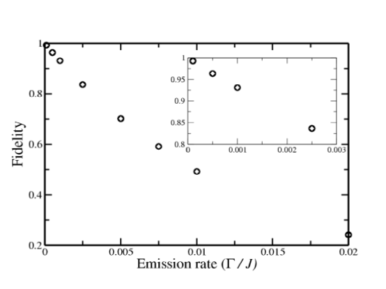
Figure 12: Fidelity simulation for CNOT gate, subject to emission errors, for a linear quantum dot array, where three physical qubits encodes each logical qubit. $\circ$ Nineteen exchange gate implementation of CNOT gate. $\diamond$ Free system evolution for duration equivalent to CNOT.

The effects of emission upon the CNOT gate fidelity are summarized in Fig. 12. We see here a greater degeneration as a function of the emission error rate. Emission events are intrinsically more detrimental to the proper operation of our quantum device than are dephasing errors. They signify a change in the system’s overall energy. In contrast, dephasing errors merely introduce a random phase difference between the ground and excited states. Note, under the independent error model used here the logical basis states do not lie in a decoherence free subspace, which would have been the case for a collective error model.⁽Bacon et al. (1999) Thus, both emission errors and dephasing errors will take the system outside the encoded subspace ($S_{z}^{tot}=1/2$). We recall that emission events are generally a much rarer occurrence than dephasing events. As mentioned in section  IV.3, the expected ratio of dephasing to emission in semiconductor quantum dots is $\frac{\Gamma_{dep}}{\Gamma_{emi}}=\frac{1/T_{2}}{1/T_{1}}\simeq 10^{2}\>-\>10^{3}$. In contrast, for $\hbar\Gamma_{dep}/J_{0}\sim 10^{-3}$ we have $\hbar\Gamma_{emi}/J_{0}\sim 10^{-5}-10^{-6}$. As seen in Fig. 12 (inset), in this regime the encoded gate fidelity is $\geq\,95\,\%$.

V.2 Algorithmic Fidelity of Three qubit Deutsch-Josza

For the the three qubit Deutsch-Josza algorithm there are eight possible function evaluations, listed in Fig. 9 (Sec. III).

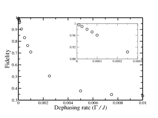
Figure 13: Simulation of three qubit Deutsch-Josza algorithm, where the fidelity plotted is the worst case fidelity, i.e the lowest calculated fidelity for any of the eight possible functions.

We found an algorithmic fidelity $F\>\geq\>0.70$ for dephasing rates $\hbar\Gamma_{dep}/J_{0}\>\leq\>10^{-3}$ (increasing to $F\,\geq\,0.98$ for $\hbar\Gamma_{dep}/J_{0}\>\leq\>10^{-5}$). The algorithmic fidelity is shown as a function of $\hbar\Gamma_{dep}/J_{0}$ in Fig. 13.

V.3 Using N-qubit unitaries to simplify algorithm implementation

From the perspective of quantum computing, another approach to overall time reduction is possible. As noted in Refs. Sanders et al., 1999 and Niskanen et al., 2003, any sequence of logical gates may be replaced by a single N-qubit unitary. Thus, in Sec. II it was shown that the sequence of four adjacent qubit CNOTs is equivalent to CNOT(1,3).We may similarly reduce combinations of other single and two qubit-gates to just one N-qubit gate involving only 2 body interactions. Certainly, many of these N-qubit gates will not be as simple as the CNOT(1,3). They may nevertheless allow for a faster, more efficient experimental realization of certain combinations of gates.

We have analyzed this approach for the example of a CNOT sandwiched between 4 Hadamard gates (Fig. 14). This circuit, which can readily be verified to be equivalent to a CNOT with the control and target qubits reversed,

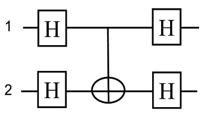
Figure 14: The 2-qubit unitary consisting of a CNOT sandwiched between 4 Hadamards.

constitutes a relatively simple two-qubit unitary where it is possible to find an analytic solution for exchange-only implementation, using the quaternion decomposition described in Appendix A. Starting with the original unreduced version ($3+1+1+3+19+3+3=33$ exchange gates) of the exact analytic CNOT sequence shown in Fig. 6, the exchange gates corresponding to the Hadamard gates are then added before and after this sequence to arrive at a 45 exchange gate sequence for the desired 2-qubit unitary, shown in Fig. 15(a)). The length of this sequence can be reduced by using the relation $H^{2}=I$ for the Hadamard gate and by combining the gate times for consecutive exchange gates acting on the same qubit pair, as was done for Fig. 6. This yields the 31 exchange gate long sequence shown in Fig. 15(b). The corresponding exchange gate times are listed in Table 3.

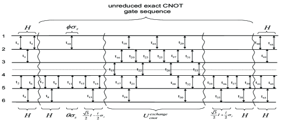
(a) Adding the exchange-only representation of the Hadamard gates onto the exact CNOT sequence of Fig. 6 results in a 45 gate exchange sequence that implements the 2-qubit unitary of Fig. 14. This sequence can be reduced by adding the gate times for consecutive exchanges acting on the same qubit pair and by making use of the relation $H^{2}=I$ for the Hadamard gate to arrive at sequence b) below.

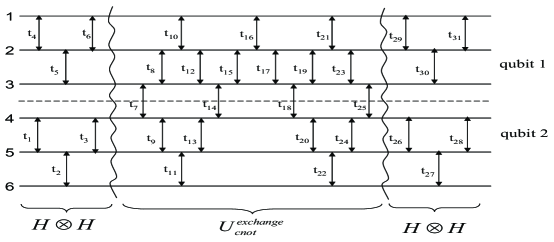
(b) Resulting shorter sequence of 31 exchange gates that directly implements the 2-qubit unitary of Fig. 14. The corresponding gate times are given in Table 3.

Figure 15:

In more general cases of $N$-qubit unitaries involving many consecutive two-qubit and one-qubit gates, this analytic approach might not be feasible and numerical optimization techniques such as that described in Section II.1 will then have to be used.

The sequence of gates shown in Fig. 15 contains 31 gates. This analytic solution should be compared against the 42 gates required for implementing the gates consecutively using $4\,\times\,3$ exchange gates to represent the four Hadamard gates and 30 exchange gates to represent the CNOT. One expects that with fewer gates and shorter total implementation time, better fidelities would result.

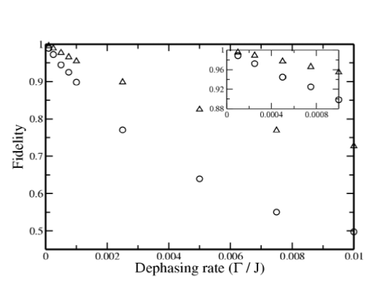
Figure 16: Comparison of fidelity obtained using a standard serial implementation of the logical gates with 42 exchange operations, versus the 31 gate sequence shown in Fig. 15. The simulations employed 20 time steps per exchange gate and 25600 trajectories averaged over at least 64 input states sampled from the surface of the hyperdimensional logical Bloch sphere, Eq. 17. Open circles ($\circ$): the normal serial implementation of the logical gates in Fig. 14 (42 exchanges). Open triangles ($\bigtriangleup$): the overall unitary gate is decomposed into individual exchange gates according to Fig. 15 (31 exchanges).

Fig. 16 shows that this is indeed the case. The fidelity for the shorter sequence is about 5 to 10 percent better at decoherence rates ($\hbar\Gamma_{dep}/J_{0}$) $\sim\,10^{-3}$, and the improvement is even greater for faster decoherence rates.

VI Summary and conclusions

We have investigated here the merits of exchange-only quantum computation based on a linear quantum dot array. For this architecture, we have shown that it is possible to achieve fidelities of 95 $\%$ or greater for the CNOT gate with realistic choices of system parameters. We have also elucidated the performance under dephasing of the 3 qubit Deutsch-Josza algorithm that is implemented with a 3 qubit encoding. For this algorithm we obtained a fidelity of at least 0.70 for realistic dephasing rates, $\hbar\Gamma_{dep}/J_{0}\leq 10^{-3}$. In addition, we have provided an example and supporting simulation data for replacing a series of gates with a single unitary. This approach is advantageous because it reduces the total time for implementing the algorithm, and will thus thereby also reduce the effects of decoherence.

Our results indicate that, due to the currently rather high decoherence rates, achieving the $10^{-4}$ threshold required for fault tolerance is beyond present capabilities in this spin-coupled quantum dot model. Nevertheless, the success probabilities for the Deutsch-Josza simulations imply that exchange coupled quantum dot arrays make for an interesting testbed. With improved experimental solid state technology, greater gate fidelities can be expected. Getting to $\hbar\Gamma_{dep}/J_{0}\,=\,10^{-5}$ will yield $\geq 98\,\%$ algorithmic fidelity (Fig. 13). In the context of extending the relevance of these simulations, and how they pertain to other systems, it should be noted that a perfectly isotropic interaction is not a necessity for universality, as it has recently been shown that both the anisotropic and asymmetric interactions are universal under appropriate encoding.⁽Vala and Whaley (2002)⁾

We have attempted to provide here a realistic estimate of gate and algorithmic fidelity for exchange-only quantum computation. Our estimates could be improved by having more realistic single spin parameters and by incorporating pulse shaping techniques. The square pulses assumed here provide only an approximation to experimental pulses. However, since the ability to implement $SU(4)$ and $SU(2)$ operations is only dependent on integrated pulse shape, square pulses are adequate from a theoretical perspective, provided that the qubit is defined on a pure two-level system and a square pulse therefore cannot cause excitation to higher levels. In the future it would be desirable to perform simulations where the pulses better reflect what is achievable in the laboratory. Allowing for pulse shaping and employing chirped pulses have been shown to improve both gate and algorithmic fidelities⁽Chen et al. (2001)⁾, making such simulations doubly interesting for future work.

VII Acknowledgments

We thank David Bacon, Kenneth Brown, and Patrick Huang for useful discussions. The effort of the authors is sponsored by the Defense Advanced Research Projects Agency (DARPA) and the Air Force Laboratory, Air Force Material Command, USAF, under Contract No. F30602-01-2-0524, and DARPA and the Office of Naval Research under grant No. FDN 00014-01-1-0826. Additional support was provided by the National Security Agency under contracts DAAD 19-00-1-0380 and DAAG 55-98-1-0371. We also thank NPACI for a generous allocation of supercomputer time at the San Diego Supercomputer Center.

Appendix A Quaternions

First developed by Hamilton, quaternions provide an alternative to the normal matrix representation of vectors and rotations in $SO(3)$.⁽Hamilton (1967); Kuipers (1998)⁾

A general quaternion, $q=\{w,q_{x},q_{y},q_{z}\}=\{w,\underline{u}\}$, is just a four component array which can represent either a vector in $\Re^{3}$ or an $SO(3)$ rotation. The first component represents a scalar and the last three components a vector. More specifically, vectors and rotations take the form:

$$v = \{0,\,v_{x},\,v_{y},\,v_{z}\}$$

$$q_{r} = \{cos(\alpha/2),\;r_{x}sin(\alpha/2),\;r_{y}sin(\alpha/2),\;r_{z}sin(\theta/2)\}$$ (32)

Here $q_{r}$ corresponds to a rotation of $\alpha$ around the Cartesian vector $\hat{r}=(r_{x},\,r_{y},\,r_{z})$. Using hyperspherical coordinates this vector, and the resulting quaternion, can be written as

$$\hat{r} = (sin(\beta/2)cos(\gamma/2),\,sin(\beta/2)sin(\gamma/2),\,cos(\beta/2))$$

$$q_{r} = \{cos(\alpha/2),\,sin(\alpha/2)sin(\beta/2)cos(\gamma/2),$$ (33)

$$sin(\alpha/2)sin(\beta/2)sin(\gamma/2),\,sin(\alpha/2)cos(\beta/2)\},$$

where $\beta$ and $\gamma$ define the axis of rotation, as shown in figure 17, and $\alpha$ is the angle of rotation around this axis.

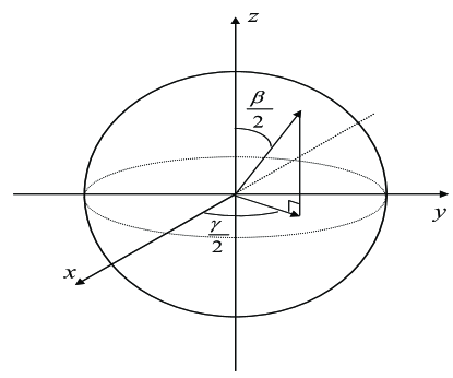
Figure 17: The angles $\beta$ and $\gamma$ are used to define the axis of rotation when using hyperspherical coordinates.

Two quaternions are multiplied together to form a new quaternion:

$$q_{1}*q_{2} = \{w_{1},\underline{u}_{1}\}*\{w_{2},\underline{u}_{2}\}$$ (34)

$$= \{w_{1}w_{2}-\underline{u}_{1}\cdot\underline{u}_{2},w_{1}\underline{u}_{2}+w_{2}\underline{u}_{1}+\underline{u}_{1}\times\underline{u}_{2}\}.$$

Hence one can derive expressions for sequences of rotations, $Q=q_{N}*q_{N-1}*...*q_{2}*q_{1}$. For example the sequence of Euler angle rotations⁽Zare (1988)⁾ $R(\phi,\theta,\chi)=e^{(-iS_{z}\phi)}e^{(-iS_{y}\theta)}e^{(-iS_{z}\chi)}$ becomes in the quaternion representation:

$$q(\phi,\theta,\chi) = \{cos(\frac{\theta}{2})cos(\frac{\phi}{2}+\frac{\chi}{2}),\,sin(\frac{\theta}{2})sin(\frac{\chi}{2}-\frac{\phi}{2}),$$ (35)

$$sin(\frac{\theta}{2})cos(\frac{\chi}{2}-\frac{\phi}{2}),\,cos(\frac{\theta}{2})sin(\frac{\chi}{2}+\frac{\phi}{2})\}.$$

The Heisenberg Hamiltonian provides us with two rotations on the encoded qubit, $\sigma_{z}$ and $\sigma_{x}$:⁽Kempe et al. (2001)⁾

$$e^{itE_{12}} = e^{-it\sigma_{z}}$$

$$e^{itE_{23}} = \ e^{it(\frac{\sqrt{3}}{2}\sigma_{x}+\frac{1}{2}\sigma_{z})}.$$ (36)

The first is a rotation around $\hat{z}$, the second a rotation around the axis $\hat{k}=\sqrt{3}/2\,\hat{x}+1/2\,\hat{z}$. Note, as seen from Eq. 2, using $E_{ij}$ rather than $H_{ij}$ to calculate gate sequences and gate times just results in a global phase in the final state, which can be accounted for as follows:

$$\prod_{k=1}^{M}\exp{(it^{\prime}_{k}E_{i_{k}j_{k}})}=\exp{(iJ_{0}/4\hbar\sum_{k=1}^{M}t_{k})}\prod_{k=1}^{M}\exp{(it_{k}H_{i_{k}j_{k}}/\hbar)}.$$ (37)

Where $t^{\prime}_{k}=\frac{J_{0}}{2\hbar}t_{k}$ results from the rescaling necessary when using $E_{ij}$ instead of $H_{ij}$.

Given the mapping of $SU(2)$ to $SO(3)$ (the Bloch sphere representation for spin-1/2 systems, see Fig. 18)⁽Sakurai (1994)⁾, these exchange gates (Eq. 36) can be cast in the quaternion representation respectively as

$$q_{1}(t) = \{cos(t/2),\,0,\,0,\,-sin(t/2)\},$$

$$q_{2}(t) = \{cos(t/2),\,\frac{\sqrt{3}}{2}sin(t/2),\,0,\,\ \frac{1}{2}sin(t/2)\}.$$ (38)

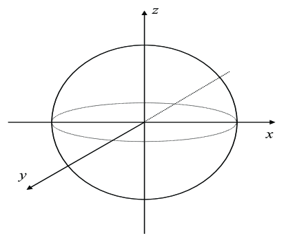
Figure 18: The Bloch sphere representation of a spin $1/2$ particle.⁽Sakurai (1994)⁾

Having obtained the quaternions that correspond to the different possible exchange gates on our encoding, and understanding how these quaternions can be multiplied together, we can now investigate the number of exchanges required to generate certain single qubit gates.

Using the geometric representation for generation of the $SU(2)$ group of rotations⁽D’Alessandro (2001); Zhang (2003)⁾ we investigate how many sequential implementations of our exchange gates, $\exp{(itE_{12})}$ and $\exp{(itE_{23})}$, suffice to generate all possible single qubit rotations. Projected onto the $x-z$ plane of the Bloch sphere, the rotations around $\hat{z}$ and $\sqrt{3}/2\,\hat{x}+1/2\,\hat{z}$ corresponding to these exchange gates can be represented as in Fig. 19.

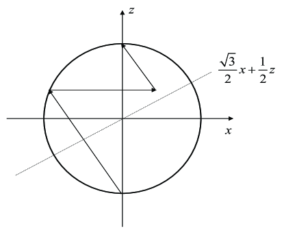
Figure 19: Planar projection of the Bloch sphere onto the $x-z$ plane, depicting the rotations corresponding to $\exp{(itE_{12})}$ and $\exp{(itE_{23})}$. Implementing $E_{12}$ is the same as rotating around the $\hat{z}$ axis, the action of which causes states to follow a line parallel to the $\hat{x}$ axis. The $E_{23}$ gate corresponds to rotations around the axis$\sqrt{3}/2\,\hat{x}+1/2\,\hat{z}$, and states then follow a line perpendicular to this axis during the duration of the gate. Combined in the sequence $\exp{(it_{3}E_{23})}\exp{(it_{2}E_{12})}\exp{(it_{1}E_{23})}$ these two exchange gates allows us to reach any point on the Bloch sphere starting from any arbitrary point. The figure shows how this sequence of gates allows us to rotate a state from the south pole to the north pole, i.e. to the most distant state. The ability to generate all other rotations follows directly from this.⁽Zhang (2003)⁾ Note, once at the north pole it might be necessary to adjust the phase of the state. Thus we need to add one more $E_{12}$ gate to the sequence, arriving at a total of at most 4 exchange gates to generate any $SU(2)$ operation. (Note that this final $E_{12}$ gate serves exactly the same purpose as the final $\sigma_{z}$ rotation does in the Euler construction.)

Based on this geometric interpretation for the action of the exchange gates, we can proceed as in Ref. Zhang, 2003 and determine the minimum number of exchange gates required to generate any $SU(2)$ rotation from a given pair of exchanges. To do this we consider how many exchange gates, and in what order they should be arranged, suffice to rotate a state from the south pole all the way to the north pole. As shown in Fig. 19, this extreme rotation can be achieved using 3 exchange gates in the sequence $\exp{(it_{3}E_{23})}\exp{(it_{2}E_{12})}\exp{(it_{1}E_{23})}$. This rotation from one pole to the other is the hardest to achieve, in the sense that it requires the most changes of direction and hence the greatest number of exchanges. All other rotations will require equal or less exchanges.⁽Zhang (2003)⁾ To this sequence of 3 exchange gates we now add a fourth exchange gate, namely $\exp{(it_{4}E_{12})}$ in order to allow for an arbitrary phase to be obtained when the state is located at the north pole of the Bloch sphere. This extra gate corresponds to the first $\sigma_{z}$ rotation when a similar decomposition is considered for the Euler angle construction for rotations in $SU(2)$ (Eq. 35). We now use the quaternion approach to find explicit exchange sequences for several elementary gates.

i) Similarity transformation for exact CNOT, S. In Section II.1) it was shown that $U_{cnot}^{exchange}$ was diagonalized as $D=S^{\dagger}U_{cnot}^{exchange}S$. Here $S=I\otimes\frac{\sqrt{3}}{2}I-\frac{i}{2}\sigma_{y}$ which corresponds to a rotation of $60^{o}$ about the y axis on the second qubit. The action of $S$ on the second qubit can be written as $cos(\frac{\pi/3}{2})I-i\,sin(\frac{\pi/3}{2})\sigma_{y}$. Referring to Eq. 33, it is evident that in the quaternion representation of rotations in $SO(3)$ this corresponds to

$$q=\{\frac{\sqrt{3}}{2},\,0,\,\frac{1}{2},\,0\}$$ (39)

For sequential application of two exchange gates, $\exp{(it_{2}E_{12})}\exp{(it_{1}E_{23})}$ or $\exp{(it_{2}E_{23})}\exp{(it_{1}E_{12})}$, consideration of the trigonometric equations that define the different components of the resulting quaternions shows that with just two exchange gates it is impossible to satisfy the requirement that both the $x$ component and $z$ component of the resulting quaternion be simultaneously zero (Eq. 39). However, with a sequence of three exchange gates ($\exp{(it_{3}E_{12})}\exp{(it_{2}E_{23})}\exp{(it_{1}E_{12})}$), which in the quaternion representation corresponds to

$$q_{S}(t_{1},t_{2},t_{3}) = \{cos(t_{2})cos(t_{1}+t_{3})\ +\frac{1}{2}sin(t_{2})sin(t_{1}+t_{3}),$$ (40)

$$\frac{\sqrt{3}}{2}sin(t_{2})cos(t_{1}-t_{3}),$$

$$\frac{\sqrt{3}}{2}sin(t_{2})sin(t_{1}-t_{3}),$$

$$-cos(t_{2})sin(t_{1}+t_{3})\ +\frac{1}{2}sin(t_{2})cos(t_{1}+t_{3})\},$$

we find that a solution for $S$ can be obtained. This is accomplished as follows. We need the $x$ component of $q_{S}$ to be zero and the $y$ component non-zero (Eq. 39). Thus we set $t_{1}-t_{3}=\pi/2$ and solve for $t_{2}$ from

$$\frac{\sqrt{3}}{2}sin(t_{2})=\frac{1}{2}.$$ (41)

We then use the first (scalar) component of $q_{S}$ to solve for $t_{1}+t_{3}$ from

$$\sqrt{\frac{2}{3}}cos(t_{1}+t_{3})+\ \frac{1}{2\sqrt{3}}sin(t_{1}+t_{3})=\frac{\sqrt{3}}{2},\\$$

which can be rewritten as

$$\frac{2}{3}\left(1-\epsilon^{2}\right)=\left(\ \frac{\sqrt{3}}{2}-\frac{\epsilon}{2\sqrt{3}}\right)^{2},$$ (42)

where $\epsilon=sin(t_{1}+t_{3})$. Solutions of Eqs. 41 and 42 yields $t_{1}=asin(1/3)/2+\pi/4$, $t_{2}=asin(1/\sqrt{3})$, and $t_{3}=asin(1/3)/2-\pi/4$.

After obtaining the three-exchange representation of $S$, we still have to find the single qubit gates that transforms the resulting matrix $D$ into the C-PHASE gate. Since C-PHASE, like $D$, is diagonal in the computational basis, a combination of $\sigma_{z}$ rotations and a global phase is sufficient to transform one into the other. To find the relevant rotation angles, $\phi$ and $\theta$ (Fig. 5(a)), and the global phase factor, $\Omega$, we set up the following system of equations

$$\Omega+\theta+\phi+\Delta_{00} = 0$$

$$\Omega+\theta-\phi+\Delta_{01} = 0$$

$$\Omega-\theta+\phi+\Delta_{10} = 0$$

$$\Omega-\theta-\phi+\Delta_{11} = \pi.$$ (43)

Here the $\Delta_{ij}$’s are the arguments of the diagonal matrix elements of $D$ when these are written as phases, i.e. $\exp(i\Delta_{ij})=D_{ij}$, and the other terms on the left are obtained from the diagonal elements of the matrix $\exp{(i\Omega)}exp{(i(\theta\,\sigma_{z}\otimes I+\phi\,I\otimes\sigma_{z}))}$. Solving for these variables, one finds that $\phi=0.612497$ and $\theta=-0.547580$. To recast these in terms of exchange gates it is enough to realize that implementing $E_{12}$ is equivalent to a $\sigma_{z}$ rotation (see Eq. 36). Thus, the exchange gate times corresponding to $\theta$ and $\phi$ are $t_{\theta}=\theta$ and $t_{\phi}=\phi$, respectively. For the $\pi/8$ gate the same argument trivially yields a single exchange gate time of $t_{\pi/8}=\pi/8$.

ii) Hadamard gate. Using the same sequence of three exchange gates, $\exp{(it_{3}E_{12})}\exp{(it_{2}E_{23})}\exp{(it_{1}E_{12})}$, and realizing that for the Hadamard gate it is the $y$ component of the resulting quaternion that must be zero, we can find the solution for the Hadamard gate in an identical fashion. This results in a quaternion representation:

$$q_{H}\left(t_{1},\,t_{2},\,t_{3}\right)=q_{H}\left(-atan(\sqrt{2})/2,\,asin(\sqrt{2/3}),\,-atan(\sqrt{2})/2\right).$$ (44)

iii) NOT gate. The NOT gate has a quaternion representation

$$q_{N}=\{0,\,1,\,0,\,0\}$$ (45)

which corresponds to a full rotation from the south pole to north, or vice versa, when interpreted on the Bloch sphere. For this gate the three exchange gate sequence considered above is insufficient to generate the gate, since this sequence can never result in an $x$ component greater than $\sqrt{3}/2$ (see Eq. 40), whereas the NOT gate requires an $x$ component of $1$. We can find a solution for the NOT gate using the modified three exchange gate sequence $\exp{(it_{3}E_{23})}\exp{(it_{2}E_{12})}\exp{(it_{1}E_{23})}$. This sequence leads to the following expression for the corresponding quaternion:

$$q_{N}(t_{1},t_{2},t_{3}) = \{cos(t_{2})cos(t_{1}+t_{3})\ +\frac{1}{2}sin(t_{2})sin(t_{1}+t_{3}),$$ (46)

$$\frac{\sqrt{3}}{2}cos(t_{2})sin(t_{1}+t_{3})\ +\frac{\sqrt{3}}{2}sin(t_{1})sin(t_{2})sin(t_{3}),$$

$$-\frac{\sqrt{3}}{2}sin(t_{2})sin(t_{1}-t_{3}),$$

$$-\frac{1}{2}sin(t_{2})cos(t_{1}-t_{3})\ +\frac{1}{2}cos(t_{2})sin(t_{1}+t_{3})$$

$$-\frac{1}{2}cos(t_{1})sin(t_{2})cos(t_{3})\},$$

We can then solve for the times $t_{s}$, $s=1\,-\,3$, by first recognizing that since the $y$ component must equal $0$ and the $x$ component must equal $1$ then, $t_{1}-t_{3}=0$. Making use of this and the expressions for the $x$ and $z$ components, we can then solve for $t_{2}$ from $t_{2}=asin(1/\sqrt{3})$. Substituting this back into the expression for the scalar component, which also must be equal to zero, we then obtain the corresponding values for $t_{1}$ and $t_{3}$ as $t_{1}=t_{3}=atan(\sqrt{2})$.

Table 1: Exchange gate times for the full sequence for CNOT in the computational basis, Eq. 6, determined by numerical optimization. Exchanges 1-8 correspond to $U_{1}\otimes U_{2}$, exchanges 9-27 to $U_{cnot}^{exchange}$, and exchanges 28-35 to $V_{1}\otimes V_{2}$ (see Fig. 4). Starting from the gate times for exchanges 9-27 given in Ref. DiVincenzo et al., 2000, a Nelder-Mead optimization routine was used to find the additional gate times corresponding to gates 1-8 and 28-35. The optimization criteria was minimization of the the cost function of Eq. 7 over the 16-dimensional parameter space of exchanges 1-8 and 28-35. The sequence of 35 gates and associated gate times seen here represent the first successful run where the cost function dropped below the required tolerance of $10^{-4}$. All gate times are given as positive numbers modulo $\pi$, in units of $2\hbar/J_{0}$.

Exchange	Qubit	Qubit		Exchange	Qubit	Qubit
Number	1	2	Time	Number	1	2	Time
1	1	2	2.462204	19	2	3	1.302882
2	2	3	0.977712	20	3	4	0.463868
3	1	2	2.209031	21	2	3	2.554511
4	2	3	0.977711	22	4	5	0.871873
5	4	5	0.690514	23	1	2	1.249644
6	5	6	2.837899	24	5	6	2.107472
7	4	5	2.298306	25	2	3	2.554511
8	5	6	1.411241	26	4	5	0.871873
9	3	4	1.290877	27	3	4	1.290877
10	2	3	0.650655	28	1	2	0.727495
11	4	5	0.871873	29	2	3	1.761338
12	1	2	1.934484	30	1	2	0.368173
13	5	6	2.107472	31	2	3	1.761338
14	2	3	0.650656	32	4	5	2.820908
15	4	5	0.871873	33	5	6	3.709248
16	3	4	2.012206	34	4	5	0.090528
17	2	3	1.302882	35	5	6	1.622010
18	1	2	2.639495

Table 2: Exchange gates and times required to transform the exchange CNOT gate into the exact CNOT gate in the computational basis, Eq. (6), obtained with analytic solution of the local transformations $U_{i},V_{i},i=1,2$. Exchange gates 1-6 correspond to $U_{1}\otimes U_{2}$, exchange gates 7-25 to $U_{cnot}^{exchange}$, and exchange gates 26-30 to $V_{1}\otimes V_{2}$ (see Fig. 6). Exchanges 7-25 are taken from Ref. DiVincenzo et al., 2000. The remaining gates (1-6 and 26-30) were arrived at analytically by decomposing each local unitary into a sequence of simpler rotations as described in the text, and then using the quaternion representation to find the corresponding rotations in $SO(3)$. See Appendix A for full details. All gate times are given as positive numbers modulo $\pi$, in units of $2\hbar/J_{0}$.

Exchange	Qubit	Qubit		Exchange	Qubit	Qubit
Number	1	2	Time	Number	1	2	Time
1	4	5	2.663935	16	1	2	2.639495
2	5	6	0.955317	17	2	3	1.302882
3	1	2	0.612498	18	3	4	0.463868
4	4	5	1.161038	19	2	3	2.554511
5	5	6	2.526113	20	4	5	0.871873
6	4	5	0.615480	21	1	2	1.249644
7	3	4	1.290877	22	5	6	2.107472
8	2	3	0.650655	23	2	3	2.554511
9	4	5	0.871873	24	4	5	0.871873
10	1	2	1.934484	25	3	4	1.290877
11	5	6	2.107472	26	4	5	2.526113
12	2	3	0.650656	27	5	6	0.615480
13	4	5	0.871873	28	4	5	0.477659
14	3	4	2.012206	29	5	6	0.955317
15	2	3	1.302882	30	4	5	2.663935

Table 3: One possible set of exchange gates and times that implements the two-qubit unitary of a CNOT sandwiched between four Hadamards (Fig. 14, equivalent to a CNOT with target and control qubits reversed). Starting with the 19-gate exchange-only CNOT sequence for $U_{cnot}^{exchange}$ of Ref. DiVincenzo et al., 2000, the additional local gates were then determined analytically using the quaternion formulation summarized in Appendix A. All gate times are given as positive numbers modulo $\pi$, in units of $2\hbar/J_{0}$.

Exchange	Qubit	Qubit		Exchange	Qubit	Qubit
Number	1	2	Time	Number	1	2	Time
1	4	5	1.638696	17	2	3	1.302882
2	5	6	2.526113	18	3	4	0.463868
3	4	5	0.615480	19	2	3	2.554511
4	1	2	2.663935	20	4	5	0.871873
5	2	3	0.955317	21	1	2	1.249644
6	1	2	0.134839	22	5	6	2.107472
7	3	4	1.290877	23	2	3	2.554511
8	2	3	0.650655	24	4	5	0.871873
9	4	5	0.871873	25	3	4	1.290877
10	1	2	1.934484	26	4	5	2.526113
11	5	6	2.107472	27	5	6	0.615480
12	2	3	0.650656	28	4	5	0.955317
13	4	5	0.871873	29	1	2	2.663935
14	3	4	2.012206	30	2	3	0.955317
15	2	3	1.302882	31	1	2	2.663935
16	1	2	2.639495

References

- DiVincenzo et al. (2000) D. P. DiVincenzo, D. Bacon, J. Kempe, G. Burkard, and K. B. Whaley, Nature 408, 339 (2000).
- Kempe et al. (2001) J. Kempe, D. Bacon, D. A. Lidar, and K. B. Whaley, Phys. Rev. A 63, 042037 (2001).
- Bacon et al. (2000) D. Bacon, J. Kempe, D. Lidar, and K. Whaley, Phys. Rev. Lett. 85, 1758 (2000).
- Landauer (1996) R. Landauer, Science 272, 1914 (1996).
- Barenco et al. (1995) A. Barenco, D. Deutsch, and A. Ekert, Phys. Rev. Lett. 74, 4083 (1995).
- Loss and DiVincenzo (1998) D. Loss and D. P. DiVincenzo, Phys. Rev. A 57, 120 (1998).
- Loss et al. (1998) D. Loss, D. P. DiVincenzo, and D. Loss, Superlattices and Microstructures 23, 419 (1998).
- Burkard et al. (1999) G. Burkard, D. Loss, and D. P. DiVincenzo, Phys. Rev. B 59, 2070 (1999).
- Kikkawa et al. (1997) J. M. Kikkawa, I. P. Smorchkova, N. Samarth, and D. D. Awschalom, Science 277, 1284 (1997).
- Fujisawa et al. (2001) T. Fujisawa, Y. Tokura, and Y. Hirayama, Phys. Rev. B 63, 081304 (2001).
- Livermore et al. (1996) C. Livermore, C. H. Crouch, R. M. Westervelt, K. L. Campman, and A. C. Gossard, Science 274, 1332 (1996).
- Tarucha et al. (1996) S. Tarucha, D. G. Austing, T. Honda, R. J. van der Hage, and L. P. Kouwenhoven, Phys. Rev. Lett. 77, 3613 (1996).
- Gupta et al. (1999) J. A. Gupta, D. D. Awschalom, X. Peng, and A. P. Alivisatos, Phys. Rev. B 59, 10421 (1999).
- Wiseman et al. (2001) H. Wiseman, D. W. Utami, H. B. Sun, G. Milburn, B. E. Kane, A. Dzurak, and R. G. Clark, Phys. Rev. B 63, 235308 (2001).
- Engel and Loss (2001) H.-A. Engel and D. Loss, Phys. Rev. Lett. 86, 4648 (2001).
- DiVincenzo (1999) D. P. DiVincenzo, Jour. Appl. Phys. 85, 4785 (1999).
- Vala and Whaley (2002) J. Vala and K. B. Whaley, Phys. Rev. A 66, 022304 (2002).
- Bonesteel et al. (2001) N. Bonesteel, D. Stepanenko, and D. DiVincenzo, Phys. Rev. Lett. 87, 207901 (2001).
- Makhlin (2002) Y. Makhlin, Quant. Info. Proc. 1, 243 (2002).
- Nielsen and Chuang (2000) M. Nielsen and I. Chuang, Quantum Computation and Quantum Information (Cambridge University Press, Cambridge, UK, 2000).
- Nelder and Mead (1965) J. Nelder and R. Mead, Computer Journal 7, 308 (1965).
- Lagarias et al. (1995) J. C. Lagarias, J. A. Reeds, M. H. Wright, and P. E. Wright, SIAM J. Optim. 9, 113 (1995).
- Sakurai (1994) J. Sakurai, Modern Quantum Mechanics (Addison-Wesley, US, 1994).
- Dalibard et al. (1992) J. Dalibard, Y. Castin, and K. Mølmer, Phys. Rev. Lett. 68, 580 (1992).
- Mølmer et al. (1993) K. Mølmer, Y. Castin, and J. Dalibard, J. Opt. Soc. Am. B 10, 524 (1993).
- Hegerfeldt and Wilser (1991) G. C. Hegerfeldt and T. S. Wilser, in Proceedings of the Second International Wigner Symposium, edited by H. Doebner, W. Scherer, and J. F. Schroeck (World Scientific, Singapore, 1991), p. 104.
- Carmichael (1993) H. Carmichael, An open systems approach to quantum optics, Lecture notes in physics (Springer, Berlin, 1993).
- Awschalom and Kikkawa (1999) D. D. Awschalom and J. M. Kikkawa, Phys. Today 52, 33 (1999).
- Zhang and Whaley (1991) Q. Zhang and K. B. Whaley, Phys. Rev. B 43, 11062 (1991).
- Zhang and Whaley (1992) Q. Zhang and K. B. Whaley, Jour. Chem. Phys. 96, 5318 (1992).
- Hahn (1950) E. Hahn, Phys. Rev. 80, 580 (1950).
- Bacon et al. (1999) D. Bacon, D. Lidar, and K. Whaley, Phys. Rev. A 60, 1944 (1999).
- Sanders et al. (1999) G. Sanders, K. Kim, and W. Holton, Phys. Rev. A 59, 1098 (1999).
- Niskanen et al. (2003) A. O. Niskanen, J. J. Vartianen, and M. M. Salomaa, Phys. Rev. Lett. 90, 197901 (2003).
- Chen et al. (2001) P. Chen, C. Piermarocchi, and L. J. Sham, Physica E 10, 7 (2001).
- Hamilton (1967) W. Hamilton, The Mathematical Papers of Sir William Rowan Hamilton. (Cambridge University Press, Cambridge, UK, 1967).
- Kuipers (1998) J. Kuipers, Quaternions and Rotation Sequences: A Primer with Applications to Orbits, Aerospace, and Virtual Reality (Princeton University Press, Princeton, NJ, 1998).
- Zare (1988) R. N. Zare, Angular Momentum (John Wiley & Sons, Inc., US, 1988).
- D’Alessandro (2001) D. D’Alessandro, quant-ph/0110120 (2001).
- Zhang (2003) J. Zhang, Ph.D. thesis, University of California, Berkeley (2003).