Polarization quantum properties in type-II Optical Parametric Oscillator below threshold

Abstract

We study the far field spatial distribution of the quantum fluctuations in the transverse profile of the output light beam generated by a type II Optical Parametric Oscillator below threshold, including the effects of transverse walk-off. We study how quadrature field correlations depend on the polarization. We find spatial EPR entanglement in quadrature-polarization components: For the far field points not affected by walk-off there is almost complete noise suppression in the proper quadratures difference of any orthogonal polarization components. We show the entanglement of the state of symmetric intense, or macroscopic, spatial light modes. We also investigate nonclassical polarization properties in terms of the Stokes operators. We find perfect correlations in all Stokes parameters measured in opposite far field points in the direction orthogonal to the walk-off, while locally the field is unpolarized and we find no polarization squeezing.

PACS number(s): 42.50.Lc, 42.50.Dv, , 42.65.Sf, 42.50.Ct

I Introduction

Polarization [2] and transverse spatial [3] degrees of freedom of light beams interacting with nonlinear media have been extensively studied in the last decade. The selection of special spatial modes of the transverse profile of a light beam down-converted by a quadratic crystal provides an interesting example of a polarization entangled state [4]. In this kind of experiments [4] the fluorescence, or rate of photon pairs production, is low (single photon regime). Recently there has been an increasing interest for polarization entanglement in continuous variable regimes, where intense light beams, with high fluxes of photons, are generated. In this case the detection no longer resolves single photon events [5, 6]. The interest in such macroscopic or multiphoton systems is partly due to possible applications of continuous variables in quantum communications [7], quantum information [8], mapping from light to atomic media [9], and quantum teleportation [10]. Most works on continuous variable regimes [5, 6, 7, 8, 9, 10] are concerned only with temporal features of light beams, while our aim in this paper is to study polarization entanglement between spatial modes of intense light beams, when intensities are continuous variables.

Interesting polarization effects arise in type II phase matching, when a pump field is down-converted in a quadratic crystal in two orthogonally polarized fields [4]. Parametric down-conversion (PDC) can be increased using an intense pump pulse or by means of a resonant optical cavity. The case of an intense pump is considered in Ref. [11]. In this paper we study the situation of an optical cavity, that is a Optical Parametric Oscillator (OPO). In the OPO the fields resonate in a cavity and therefore an intense laser-like beam is down-converted above threshold. The cavity enhances the rate of production of photons pairs, increasing the gain and providing active filtering of the frequency bandwidth [12, 13]. The spatial distribution of the quantum fluctuations close to threshold is dominated by weakly damped modes that become unstable at the threshold of the OPO, as discussed in Sect.II. This fluctuating spatial structure, known as ‘quantum image’, has been extensively studied for type I OPO, where polarization does not play any important role [14, 15, 16]. Here we analyze the spatial quantum fluctuations for type II phase matching, considering the polarization and the transverse spatial degrees of freedom. We also study the effects of the transverse walk-off between the orthogonally polarized signal and idler down-converted fields.

The characterization of the spatial and polarization properties of the down-converted light is given in two different ways, discussed in Sect. III and in Sect. IV, respectively. In Sect.III we study Einstein-Podolsky-Rosen (EPR) correlations [17] between polarization-quadratures components. A precedent of macroscopic EPR experiments in OPO are those of Ref.[18, 19], but they do not refer to spatial EPR, distinguishing signal and idler by their polarization. Spatial EPR was theoretically considered in Refs. [20, 21] in type I-OPO. We build on these results by considering the polarization degree of freedom and including the walk-off effects in our treatment. Our main finding is that for the intersection points of the far field rings there is noise suppression much below the standard quantum limit in the proper quadratures combinations of any orthogonal polarization components of the critical modes. We show that the entanglement observed in single photon regime [4] survives for the multipohoton state generated by an OPO near below threshold.

In Sect.IV we analyze the issue of macroscopic polarization entanglement in terms of Stokes operators. These operators are related to the intensity of different polarization components of light. There is a recent experimental observation of polarization squeezing in three of the four Stokes parameters [22], while macroscopic polarization entanglement in terms of Stokes parameters has been considered in Ref. [5] and demonstrated in Ref. [6]. The situations considered in Refs.[22, 5, 6] do not involve transverse spatial degrees of freedom. Quantum properties of Stokes operators taking into account the spatial transverse dependence of light seem to be first considered here and in Ref. [11]. We study both the local properties of Stokes parameters in the transverse far field profile of the down-converted beam (Sect.IV A) and the possibility of entanglement between spatial far field modes (Sect.IV B). As a main result we show that there exists macroscopic polarization entanglement between the beams measured at the intersection points of the far field rings. We find perfect quantum correlation at zero-frequency in all Stokes operators.

II Input/output relations and far field characteristics

We consider a type II OPO below threshold, in the undepleted pump approximation. In this approximation the pump field is described by a fixed classical variable $A_{0}$. In the mean field approximation the signal ($\hat{A}_{1}$, ordinary $x$ polarized) and the idler ($\hat{A}_{2}$, extraordinary $y$ polarized) fields obey the following Heisenberg operator equations [15]:

$$\partial_{t}\hat{A}_{1} = -\gamma_{1}(1+i\Delta_{1}-ia_{1}\nabla^{2}+\rho_{1}{\partial_{y}})\hat{A}_{1}+\sqrt{\gamma_{1}\gamma_{2}}{A}_{0}\hat{A}_{2}^{\dagger}$$ (1)

$$+ \sqrt{2\gamma_{1}}\hat{A}_{1}^{in}$$ (2)

$$\partial_{t}\hat{A}_{2} = -\gamma_{2}(1+i\Delta_{2}-ia_{2}\nabla^{2}+\rho_{2}{\partial_{y}})\hat{A}_{2}+\sqrt{\gamma_{1}\gamma_{2}}{A}_{0}\hat{A}_{1}^{\dagger}$$ (3)

$$+ \sqrt{2\gamma_{2}}\hat{A}_{2}^{in}$$ (4)

where $\gamma_{i}$ are the cavity linewidths for the signal and idler fields, $\Delta_{i}$ are the cavity detunings, $\nabla^{2}$ is the two dimensional transverse Laplacian that models the effect of diffraction in the paraxial approximation, and $a_{i}$ are the diffraction strengths. In type II phase matching a transverse walk-off arises between the signal and idler fields. It is described by the drift terms $\rho_{i}{\partial_{y}}\hat{A}_{i}$. $\hat{A}_{i}^{in}$ are the the input field operators, describing the fluctuations of the signal and idler modes entering through the partially transmitting cavity mirror.

From the Fourier transform:

$$\hat{A}(\vec{x},t) = \int\frac{d^{2}\vec{k}}{2\pi}\int\frac{d\omega}{\sqrt{2\pi}}e^{i(\vec{k}\cdot\vec{x}-\omega t)}\hat{A}(\vec{k},\omega)$$ (5)

$$\hat{A}^{\dagger}(\vec{x},t) = \int\frac{d^{2}\vec{k}}{2\pi}\int\frac{d\omega}{\sqrt{2\pi}}e^{i(\vec{k}\cdot\vec{x}-\omega t)}\hat{A}^{\dagger}(-\vec{k},-\omega)$$ (6)

we obtain the following algebraic linear relation, giving the intracavity mode operators $\boldsymbol{\hat{\nu}(\vec{k},\omega)}$ in terms of the input fields $\boldsymbol{\hat{\nu}^{in}(\vec{k},\omega)}$

$$\boldsymbol{L}\boldsymbol{\hat{\nu}}=\boldsymbol{\Gamma}\boldsymbol{\hat{\nu}^{in}},$$ (7)

where we have introduced the operator vectors

$$\boldsymbol{\hat{\nu}}=\left(\begin{array}[]{c}\hat{A}_{1}(\vec{k},\omega)\\ \hat{A}^{\dagger}_{2}(-\vec{k},-\omega)\end{array}\right),\,\boldsymbol{\hat{\nu}^{in}}=\left(\begin{array}[]{c}\hat{A}^{in}_{1}(\vec{k},\omega)\\ \hat{A}^{in\dagger}_{2}(-\vec{k},-\omega)\end{array}\right),\,$$ (12)

and the matrices

$$\boldsymbol{L} = \left(\begin{array}[]{cc}\gamma_{1}(1+i\Delta_{1}(\vec{k},\omega))&-\sqrt{\gamma_{1}\gamma_{2}}A_{0}\\ -\sqrt{\gamma_{1}\gamma_{2}}A^{*}_{0}&\gamma_{2}(1-i\Delta_{2}(-\vec{k},-\omega))\end{array}\right),$$ (15)

$$\boldsymbol{\Gamma} = \left(\begin{array}[]{cc}\sqrt{2\gamma_{1}}&0\\ 0&\sqrt{2\gamma_{2}}\end{array}\right),\,$$ (18)

with

$$\Delta_{j}(\vec{k},\omega)=\Delta_{j}+a_{j}|\vec{k}|^{2}+\rho_{j}k_{y}-\omega/\gamma_{j}.$$ (19)

Using the input/output relations $\boldsymbol{\hat{\nu}^{out}}=\boldsymbol{\Gamma}\boldsymbol{\hat{\nu}}-\boldsymbol{\hat{\nu}^{in}}$ [23] we obtain the output fields:

$$\hat{A}^{out}_{1,2}(\vec{k},\omega)=U_{1,2}(\vec{k},\omega)\hat{A}^{in}_{1,2}(\vec{k},\omega)+V_{1,2}(\vec{k},\omega)\hat{A}^{in}_{2,1}(-\vec{k},-\omega).$$ (20)

The coefficients of the input/output transformation are:

$$U_{1}(\vec{k},\omega) = \frac{2[1-i\Delta_{2}(-\vec{k},-\omega)]}{[1+i\Delta_{1}(\vec{k},\omega)][1-i\Delta_{2}(-\vec{k},-\omega)]-|A_{0}|^{2}}-1$$ (21)

$$V_{1}(\vec{k},\omega) = \frac{2A_{0}}{[1+i\Delta_{1}(\vec{k},\omega)][1-i\Delta_{2}(-\vec{k},-\omega)]-|A_{0}|^{2}}$$ (22)

and $U_{2}$, $V_{2}$ are obtained interchanging the indexes $1$ and $2$ in Eqs. (21) and Eq. (22).

Assuming that the input signal and idler fields are in the vacuum state, it is immediate to obtain the non-vanishing second order moments of the output fields

$$\langle\hat{A}^{out~{}\dagger}_{1}(\vec{k},\omega)\hat{A}^{out}_{1}(\vec{k}^{\prime},\omega^{\prime})\rangle = |V_{1}(\vec{k},\omega)|^{2}\delta(\vec{k}-\vec{k}^{\prime})\delta(\omega-\omega^{\prime}),$$ (23)

$$\langle\hat{A}^{out~{}\dagger}_{2}(\vec{k},\omega)\hat{A}^{out}_{2}(\vec{k}^{\prime},\omega^{\prime})\rangle = |V_{2}(\vec{k},\omega)|^{2}\delta(\vec{k}-\vec{k}^{\prime})\delta(\omega-\omega^{\prime}),$$ (24)

$$\langle\hat{A}^{out}_{1}(\vec{k},\omega)\hat{A}^{out}_{2}(\vec{k}^{\prime},\omega^{\prime})\rangle = U_{1}(\vec{k},\omega)V_{2}(-\vec{k},-\omega)$$ (25)

$$\delta(\vec{k}+\vec{k}^{\prime})\delta(\omega+\omega^{\prime})$$ (26)

and the corresponding hermitian conjugate ones. From these moments, quadrature and intensity correlations can be analytically calculated for a transversally homogeneous pump $A_{0}$. These calculations can be simplified considering the unitary conditions (see, for instance, Ref. [15]) and the symmetries of the system. From Eqs.(23)-(24) we obtain the local Far Field (FF) intensity. From Eq.(25) it is evident that correlations between signal and idler are non vanishing only between symmetric points of the far field. Such two-mode correlations are due to the quadratic form of the Hamiltonian describing, within a linear approximation, the OPO below threshold. In the following, and in order to avoid unphysical divergences [24], we consider that the fields are integrated over a detection region $R_{\vec{k}}$ of area $\sigma$:

$$\hat{A}^{out}(\vec{k})\rightarrow\int_{R_{\vec{k}}}dk^{\prime}\hat{A}^{out}(\vec{k}^{\prime}).$$ (27)

At the threshold for signal generation ($A_{0}^{thr}=1$), and for a negative total detuning ($\gamma_{1}\Delta_{1}+\gamma_{2}\Delta_{2}<0$), an instability at finite wavenumber and with nonzero frequency appears, as extensively discussed in Refs. [25, 26]. The modes that become unstable at threshold are determined by the relations $\Delta_{1}(\vec{k},\omega_{H}(\vec{k}))=0$ and $\Delta_{2}(\vec{k},\omega_{H}(\vec{k}))=0$, where

$$\omega_{H}(\vec{k}) = \frac{\gamma_{1}\gamma_{2}}{\gamma_{1}+\gamma_{2}}\cdot$$ (29)

$$[\Delta_{1}-\Delta_{2}+(a_{1}-a_{2})|\vec{k}|^{2}+(\rho_{1}+\rho_{2})k_{y}]$$

is the frequency that becomes undamped at threshold (Hopf bifurcation).

The unstable critical modes lie on two rings of the far field given by:

$$\gamma_{1}\Delta_{1}+\gamma_{2}\Delta_{2}+(\gamma_{1}a_{1}+\gamma_{2}a_{2})|\vec{k}|^{2}\pm(\gamma_{1}\rho_{1}-\gamma_{2}\rho_{2})k_{y}$$ (30)

$$=0.$$ (31)

If the relative walk-off $\gamma_{1}\rho_{1}-\gamma_{2}\rho_{2}$ vanishes, Eq.(31) describes a single far field ring. Therefore in absence of walk-off the signal and the idler far field distributions are superimposed, and an intense ring is observed. The two rings of Eq.(31) are clearly identified in Fig.1, where we represent the stationary mean intensity close to threshold:

$$\langle\hat{A}^{out~{}\dagger}_{1}(\vec{k},t)\hat{A}^{out}_{1}(\vec{k},t)+\hat{A}^{out~{}\dagger}_{2}(\vec{k},t)\hat{A}^{out}_{2}(\vec{k},t)\rangle=$$ (32)

$$\frac{\sigma}{2\pi}\int d\omega(|V_{1}(\vec{k},\omega)|^{2}+|V_{2}(\vec{k},\omega)|^{2}).$$ (33)

This figure is similar to the well-known experimental image obtained when there is no cavity, in spontaneous parametric down conversion [4, 11]. We want to point out that the cavity introduces fundamental differences: in particular in the cavity case there is a threshold above which a pattern appears in the transverse profile of the fields. The modulus of the wave-vector of such pattern at threshold is identified in the noisy $precursor$ below threshold [27]. The existence of a selected wave-number is an effect of the optical cavity, its value being determined by the cavity detuning [25].

The main contribution to the integrals in Eq. (32) are the most intense frequencies components given by Eq. (29). Hence the intensity at the Hopf frequency

$$\langle\hat{A}^{out~{}\dagger}_{1}(\vec{k},\omega_{H}(\vec{k}))\hat{A}^{out}_{1}(\vec{k},\omega_{H}(\vec{k}))+$$ (34)

$$\hat{A}^{out~{}\dagger}_{2}(\vec{k},\omega_{H}(\vec{k}))\hat{A}^{out}_{2}(\vec{k},\omega_{H}(\vec{k}))\rangle$$ (35)

is very similar to the one of Fig. 1. This picture of the FF shows that the intensity reaches the highest value at the intersection points of the two rings, where ordinary and extraordinary fields are superimposed. From Eq.(31) it is immediate to obtain the coordinates of these crossing points:

$$\pm\vec{k}_{H}=(\pm k_{x}^{c},0)\textrm{, with }k_{x}^{c}=\sqrt{\frac{-\gamma_{1}\Delta_{1}-\gamma_{2}\Delta_{2}}{\gamma_{1}a_{1}+\gamma_{2}a_{2}}}.$$ (36)

In our calculations we will also consider the FF modes on the rings for which the influence of the walk-off is stronger. These are the four points of intersection of the two rings and the $y$ axis, with ordinates:

$$\pm k_{y\pm}^{c}=\frac{1}{2(\gamma_{1}a_{1}+\gamma_{2}a_{2})}\left[\pm(\gamma_{1}\rho_{1}-\gamma_{2}\rho_{2})\right.$$ (37)

$$\left.\pm\sqrt{(\gamma_{1}\rho_{1}-\gamma_{2}\rho_{2})^{2}-4(\gamma_{1}\Delta_{1}+\gamma_{2}\Delta_{2})(\gamma_{1}a_{1}+\gamma_{2}a_{2})}\right].$$ (38)

We define the two external points by $\pm\vec{k}_{V}=(0,\pm k_{y+}^{c})$, with $k_{y+}^{c}$ obtained from Eq. (37) with both $+$ signs.

For simplicity in the following we shall omit the label $out$, indicating with $\hat{A}_{1,2}$ the output fields, described by Eqs. (23)-(25).

III Spatial EPR entanglement between quadrature-polarization field components

The vectorial field is a superposition of linearly polarized components:

$$\hat{\vec{A}}=\hat{A}_{1}\vec{e}_{x}+\hat{A}_{2}\vec{e}_{y}.$$ (39)

By means of a wave retarder

$$W=\left(\begin{array}[]{cc}1&0\\ 0&e^{i\Gamma}\end{array}\right)\,$$ (42)

and a polarization rotator

$$P=\left(\begin{array}[]{cc}~{}\cos\Theta&\sin\Theta\\ -\sin\Theta&\cos\Theta\end{array}\right)\,,$$ (45)

we can obtain a field ${\hat{\vec{A}}_{\Gamma\Theta}}=WP\hat{\vec{A}}$ in any polarization state

$$\hat{\vec{A}}_{\Gamma\Theta}=(\hat{A}_{1}\cos\Theta+\hat{A}_{2}e^{i\Gamma}\sin\Theta)\vec{e}_{x}+$$ (46)

$$(-\hat{A}_{1}\sin\Theta+\hat{A}_{2}e^{i\Gamma}\cos\Theta)\vec{e}_{y}.$$ (47)

With a linear polarizer

$$L=\left(\begin{array}[]{cc}1&0\\ 0&0\end{array}\right)\,,$$ (50)

we can select a field polarization component, and, integrating over a detection region $R_{\vec{k}}$, we obtain

$$\hat{A}_{\Gamma\Theta}(\vec{k},t)=\int_{R_{\vec{k}}}d\vec{k}^{\prime}(\hat{A}_{1}(\vec{k}^{\prime},t)\cos\Theta+\hat{A}_{2}(\vec{k}^{\prime},t)e^{i\Gamma}\sin\Theta).$$ (51)

By homodyne detection we can select a quadrature component of this polarization component. We define the quadrature $\Psi$ by

$$A_{\Gamma\Theta}^{\Psi}(t)=A_{\Gamma\Theta}(t)e^{i\Psi}+(A_{\Gamma\Theta})^{\dagger}(t)e^{-i\Psi}.$$ (52)

In any FF point, the arbitrary quadrature-polarization component (52) has vanishing mean value and a spectral variance which depends only on $\Theta$, but it is independent of the choice of the phase factors $\Psi$ and $\Gamma$. Integrating over a detection region $R_{\pm\vec{k}}$ of area $\sigma$, much smaller of the variation scale of $U_{i}$ and $V_{i}$, we obtain

$$\int dte^{i\omega t}\langle\hat{A}_{\Gamma\Theta}^{\Psi}(\vec{k},t)A_{\Gamma\Theta}^{\Psi}(\vec{k},0)\rangle=$$ (53)

$$\sigma[1+\cos^{2}\Theta(|V_{1}(\vec{k},\omega|^{2}+|V_{1}(\vec{k},-\omega|^{2})+$$ (54)

$$\sin^{2}\Theta(|V_{2}(\vec{k},\omega|^{2}+|V_{2}(\vec{k},-\omega)|^{2}],$$ (55)

where $\sigma$ fixes the shot noise level. Therefore, in any far field point the variance of an arbitrary quadrature-polarization component is above the shot noise level $\sigma$. We observe that if we place the detectors in the FF line $k_{y}=0$ the variance results independent of all angles, including $\Theta$. We find

$$\int dte^{i\omega t}\langle\hat{A}_{\Gamma\Theta}^{\Psi}((k_{x},0),t)A_{\Gamma\Theta}^{\Psi}((k_{x},0),0)=$$ (56)

$$\sigma[1+|V_{1}((k_{x},0),\omega|^{2}+|V_{1}((k_{x},0),-\omega)|^{2}],$$ (57)

In other words, for $k_{y}=0$, the level of fluctuations is independent of the choice of the polarization state and quadrature, depending only on the position $k_{x}$.

Next, we consider the correlations between the field components detected from two spatially separated FF points. Such correlations are not vanishing only for symmetric FF points $\vec{k}$ and $-\vec{k}$. We will show that the correlations between quadratures measured from these two positions of the transverse plane show EPR entanglement. A two mode state is here defined to be EPR entangled if for two orthogonal quadratures $\hat{X}_{i}$ and $\hat{Y}_{i}$ in each mode $i$ ($i=1,2$) the conditional variances $V^{-}_{cond}(\hat{X}_{1}|\hat{X}_{2})$ and $V^{+}_{cond}(\hat{Y}_{1}|\hat{Y}_{2})$ are both less than $1$, as discussed in Ref.[7]. The conditional variance is defined by

$$V^{\pm}_{cond}(\hat{A}|\hat{B})=\min_{g}\frac{V(\hat{A}\pm g\hat{B})}{V(\hat{A}_{SN})}$$ (58)

being $V(\hat{A})$ the variance, and $V(\hat{A}_{SN})$ the shot noise level. The factor $g$ is introduced to optimize noise reduction and is experimentally obtained by an attenuator and a delay line [21]. We note that

$$V(\hat{X}_{1}-\hat{X}_{2}) < V(\hat{X}_{1,SN})~{}~{}\textrm{and}~{}~{}$$ (59)

$$V(\hat{Y}_{1}+\hat{Y}_{2}) < V(\hat{Y}_{1,SN})$$ (60)

is a sufficient condition for EPR entanglement, corresponding to the choice $g=1$. The definition of EPR entanglement used here [7] provides a sufficient condition for the inseparability criterion recently discussed for continuous variables systems in Ref.[29].

For a single-mode type II OPO below threshold, in which transverse effects are not considered, EPR correlations between signal and idler modes of different polarizations have been predicted and experimentally demonstrated [28]. Recent investigations show the possibility of EPR entanglement between spatial regions of the transverse profile of the signal field of a degenerate optical parametric oscillator [20, 21]. For type II phase matching we can consider two symmetric far field modes with $x$ and $y$ polarizations, respectively. Neglecting walk-off effects we would then find results equivalent to the degenerate case in type I phase matching [20, 21]. In addition of considering the effect of the walk-off, the novelty of our discussion here for type II OPO is that we can also consider how these correlations change with the polarization state.

As an indicator to look for EPR entanglement in our case, we introduce the spectral variance of the difference of quadratures

$${\mathcal{V}}_{g}(\pm\vec{k},\omega;\vec{\Phi})= \int dte^{i\omega t}\langle(\hat{A}_{\Gamma\Theta}^{\Psi}(\vec{k},t)-g^{*}\hat{A}_{\Gamma^{\prime}\Theta^{\prime}}^{\Psi^{\prime}}(-\vec{k},t))$$ (62)

$$(\hat{A}_{\Gamma\Theta}^{\Psi}(\vec{k},0)-g\hat{A}_{\Gamma^{\prime}\Theta^{\prime}}^{\Psi^{\prime}}(-\vec{k},0))\rangle,$$

where the vector $\vec{\Phi}=(\Gamma,\Theta,\Psi,\Gamma^{\prime},\Theta^{\prime},\Psi^{\prime})$ is the set of parameters determining the polarizations (lower labels) and quadratures (upper labels) of the symmetric FF modes under consideration. The value of $g$ giving the minimum variance (62) is

$$\bar{g}=\frac{\int dte^{i\omega t}\langle\hat{A}_{\Gamma^{\prime}\Theta^{\prime}}^{\Psi^{\prime}}(-\vec{k},t)\hat{A}_{\Gamma\Theta}^{\Psi}(\vec{k},0)\rangle}{\int dte^{i\omega t}\langle\hat{A}_{\Gamma^{\prime}\Theta^{\prime}}^{\Psi^{\prime}}(-\vec{k},t)\hat{A}_{\Gamma^{\prime}\Theta^{\prime}}^{\Psi^{\prime}}(-\vec{k},0)\rangle}$$ (63)

From the output moments Eqs. (23-25) we obtain

$${\mathcal{V}}_{g}(\pm\vec{k},\omega;\vec{\Phi})=\sigma$$ (64)

$$\left[|e^{i(\Psi+\Psi^{\prime}+\Gamma^{\prime})}\cos\Theta U_{1}(\vec{k},\omega)-g^{*}\sin\Theta^{\prime}V_{2}^{*}(-\vec{k},-\omega)|^{2}\right.$$ (65)

$$+\left.|e^{i(\Psi+\Psi^{\prime}+\Gamma^{\prime})}g^{*}\sin\Theta^{\prime}U_{1}(\vec{k},-\omega)-\cos\Theta V_{2}^{*}(-\vec{k},\omega)|^{2}\right.$$ (66)

$$+\left.|e^{i(\Psi+\Psi^{\prime}+\Gamma)}\sin\Theta U_{1}(-\vec{k},-\omega)-g^{*}\cos\Theta^{\prime}V_{2}^{*}(\vec{k},\omega)|^{2}\right.$$ (67)

$$+\left.|e^{i(\Psi+\Psi^{\prime}+\Gamma)}g^{*}\cos\Theta^{\prime}U_{1}(-\vec{k},\omega)-\sin\Theta V_{2}^{*}(\vec{k},-\omega)|^{2}\right]$$ (68)

with shot noise level $\sigma(1+|g|^{2})$. A variance below this shot noise level is a signature of squeezing. We are looking for the more stringent conditions (58) discussed above: EPR entanglement imposes the requirement that ${\mathcal{V}}_{g}(\pm\vec{k},\omega;\vec{\Phi})$ goes below the shot noise level of $\hat{A}_{\Gamma\Theta}^{\Psi}$ (that is we should find ${\mathcal{V}}_{g}(\pm\vec{k},\omega;\vec{\Phi})<\sigma$), simultaneously for two combinations of orthogonal quadratures [7].

The general result (64) depends on many parameters. However it is important to note that ${\mathcal{V}}_{g}$ only depends on the phases $\Psi,\Psi^{\prime},\Gamma,\Gamma^{\prime}$ through the independent combinations $(\Psi+\Psi^{\prime}+\Gamma)$ and $(\Psi+\Psi^{\prime}+\Gamma^{\prime})$. The dependence on the sum of quadratures angles $\Psi$ and $\Psi^{\prime}$ is well known in other contexts. It is easily understood taking into account that measuring by a single homodyne detector the noise in a quadrature $\frac{\Psi+\Psi^{\prime}}{2}$ of the difference of the spatial $\pm\vec{k}$ and polarization ($\Gamma,\Theta,\Gamma^{\prime},\Theta^{\prime}$) modes is equivalent to the noise measurement described by Eq.(62) [28]. The result that ${\mathcal{V}}_{g}$ depends on independent variations of $\Gamma$ and $\Gamma^{\prime}$ only through their sum with the sum of the quadrature phases $\Psi+\Psi^{\prime}$ means that it is equivalent to vary the selected quadrature changing the phase of the local oscillator or to shift both signal and idler fields by a proper phase with the phase retarders.

In order to study how correlations change in different spatial points of the FF we consider two detection schemes, with detectors in symmetric FF points, which represent possible extreme cases:

• In the first detection scheme the field is detected in the crossing points $\pm\vec{k}_{H}$ of the signal and idler rings in the FF, as represented in Fig. 2. Being these points in the line $k_{y}=0$, they are not affected by the transverse walk-off. In Fig. 2 we indicate the case in which in one point the polarization component $x$ is selected and in the symmetric point the polarization $y$ is selected. In Sect. III A we will show that for these special points of the FF any change in the selection of the polarization does not influence the results given by Eq. (64).

• In the second arrangement, shown in Fig. 3, the detectors are located in a couple of symmetric points $\pm\vec{k}_{V}$ on the line $k_{x}=0$, where the walk-off effect is more pronounced. In Sect. III B we will consider the effect of changing the polarization state selected. We can distinguish two extreme cases: Fig.3a shows the arrangement in which the most intense polarization components on the rings are detected. We name this scheme as “vertical bright scheme”. Fig.3b shows the case in which the $y$ ($x$) polarization component is selected on the intense lower (upper) $x$ ($y$) polarized ring. We name this scheme as “vertical dark scheme”.

A EPR between far field modes unaffected by walk-off

In the line $k_{y}=0$ there is no effect of the transverse walk-off and the coefficients given by Eqs.(19), (21) and (22) have the following reflection symmetry:

$$U_{j}(k_{x},k_{y}=0) = U_{j}(-k_{x},k_{y}=0)$$ (69)

$$V_{j}(k_{x},k_{y}=0) = V_{j}(-k_{x},k_{y}=0)$$ (70)

with $j=1,2$. The results presented in this section are strongly dependent on this symmetry, generally present also in previous treatments of spatial EPR correlations and squeezing.

Even with this symmetric form of the coefficients the variance given by Eq.(64) is a complicated function of many parameters. For the sake of simplicity we first consider Eq.(64) in the case of $g=1$ (see Eq.(60)). The microscopic process of generation of twin photons with linear orthogonal polarization ($\Theta=0$ and $\Theta^{\prime}=\pi/2$) suggests a natural choice for the relative phases of the polarizers. Hence we consider a case in which the polarizers in the symmetric points $\pm\vec{k}_{H}$ have a relative phase fixed by

$$\Theta^{\prime}=\Theta+\pi/2.$$ (71)

Using this relation between $\Theta^{\prime}$ and $\Theta$, Eq.(64) becomes independent of $\Theta$ for $g=1$ when the additional choice

$$\Gamma^{\prime}=\Gamma+\pi$$ (72)

is also made. With these particular choice of parameters, Eq. (64) for the $\pm\vec{k}_{H}$ points (36) reduces to:

$${\mathcal{V}}_{g=1}(\pm\vec{k}_{H},\omega;[\Gamma,\Theta,\Psi,\Gamma+\pi,\Theta+\pi/2,\Psi^{\prime}])=$$ (73)

$$\sigma\left[~{}|e^{i(\Psi+\Psi^{\prime}+\Gamma)}U_{1}(\vec{k}_{H},\omega)+V_{2}^{*}(\vec{k}_{H},-\omega)|^{2}\right.$$ (74)

$$+\left.|e^{i(\Psi+\Psi^{\prime}+\Gamma)}U_{1}(\vec{k}_{H},-\omega)+V_{2}^{*}(\vec{k}_{H},\omega)|^{2}\right].$$ (75)

Eq.(75) explicitly shows that the fluctuations in any quadrature of the difference of symmetric spatial modes $\pm\vec{k}_{H}$, with relative polarizations fixed by Eqs.(71)-(72), are independent of the choice of the polarization reference $\Theta$.

With the above motivation for the relations between phase parameters, we analyze the EPR correlations in the $\pm\vec{k}_{H}$ points (Fig. 2) fixing the parameters $\Theta=0$, $\Gamma=\pi$, $\Theta^{\prime}=\pi/2$, $\Gamma^{\prime}=2\pi$, so that $\hat{A}_{\Gamma\Theta}^{\Psi}=\hat{A}_{1}^{\Psi}$ and $\hat{A}_{\Gamma^{\prime}\Theta^{\prime}}^{\Psi^{\prime}}=\hat{A}_{2}^{\Psi}$, and varying the quadrature angles $\Psi$, $\Psi^{\prime}$. There is no loss of generality in this choice of $\Gamma$ and $\Theta$ since Eq.(75) is independent of $\Theta$, and the phase $\Gamma$ can be absorbed in the quadrature angles $\Psi+\Psi^{\prime}$. As discussed previously (see Eq.(60)), EPR entanglement is guaranteed – for some quadratures ($\Psi+\Psi^{\prime}$) – if both the ‘position’ and ‘momentum’ operators

$$\hat{A}_{1}^{\Psi}(\vec{k}_{H})-\hat{A}_{2}^{\Psi^{\prime}}(-\vec{k}_{H})=$$ (76)

$$[\hat{A}_{1}(\vec{k}_{H})e^{i\Psi}+H.c.]-[\hat{A}_{2}(-\vec{k}_{H})e^{i\Psi^{\prime}}+H.c.]$$ (77)

$$\hat{A}_{1}^{\Psi+\pi/2}(\vec{k}_{H})+\hat{A}_{2}^{\Psi^{\prime}+\pi/2}(-\vec{k}_{H})=$$ (78)

$$[i\hat{A}_{1}(\vec{k}_{H})e^{i\Psi}+H.c.]+[i\hat{A}_{2}(-\vec{k}_{H})e^{i\Psi^{\prime}}+H.c.]$$ (79)

show simultaneously a variance below the reference value $\sigma$. This value corresponds to the shot noise level of both $\hat{A}_{1}^{\Psi}(\vec{k}_{H})$ and $\hat{A}_{1}^{\Psi+\pi/2}(\vec{k}_{H})$. Using Eq. (64) it turns out that (76) and (78) have the same spectral variance. Therefore, in the following we only consider Eq. (64) normalized to the shot noise level $\sigma$ for the ‘position’ operator Eq. (76), which is identified by the angles $\vec{\Phi}=(\pi,0,\Psi,0,\pi/2,\Psi^{\prime})$.

In Fig. 4 we represent the normalized variance ${\mathcal{V}}_{g=1}(\pm\vec{k}_{H},\omega;\vec{\Phi})/{\sigma}$ for the points $\pm\vec{k}_{H}$. When this normalized variance is less than $1$, we find EPR entanglement. We see a maximum noise reduction for $\Psi+\Psi^{\prime}=0$, and for $\omega=0$. Fig.5 shows a cut of Fig.4 for $\Psi+\Psi^{\prime}=0$ (continuous black line). A variation in the quadrature angle results in a mixing of squeezed and unsqueezed quadratures degrading the entanglement: strongest degrading effects are evident at small frequency (dashed black in Fig.5).

The fact that there is maximum noise reduction for $\Psi+\Psi^{\prime}=0$ can be understood by analogy with the result for the single-mode non-degenerate OPO discussed in Ref.[28]. In fact, for the case of vanishing detunings of the signal and idler and for real pump, which was the one considered in Ref. [28], the squeezing direction corresponds to the real quadratures ($\Psi=\Psi^{\prime}=0$). In our case we find an analogous result because we are also considering a real pump, and the effective detunings, given by (19), also vanish: $\Delta_{j}(\vec{k}=\pm\vec{k}_{H},\omega=0)=0$.

Our calculations allows us to search for EPR entanglement considering any couple of symmetric FF modes (distinguished by their transversal wavevector) and selecting any polarization. We have found EPR entanglement for the modes $\pm\vec{k}_{H}$ for any choice of the polarization component in $-\vec{k}_{H}$ (varying $\Theta$), if in $+\vec{k}_{H}$ we select the orthogonal polarization ($\Theta^{\prime}=\Theta+\pi/2$). In these far field points $\pm\vec{k}_{H}$, which are not affected by the walk-off, any mixing of the the signal and idler fields detected in a point is entangled with the field in the symmetric point, if this is also properly mixed (Eqs.(71)-(72)).

So far we have considered the case $g=1$ and we have found that a sufficient condition to guarantee EPR entanglement between the modes $\pm\vec{k}_{H}$ is fulfilled (see Eq.60). If we now optimize the noise reduction considering $g=\bar{g}$ we obtain the results shown in Fig.6. Comparing the normalized variance ${\mathcal{V}}_{g=1}$ (Fig. 4) with ${\mathcal{V}}_{\bar{g}}$ (Fig. 6) we observe that with the choice $g=\bar{g}$, EPR entanglement is observed in a larger frequency bandwidth. For a more direct comparison of the variances obtained for $g=\bar{g}$ and $g=1$, both quantities are plotted for $\Psi+\Psi^{\prime}=0$ in Fig.5: for small frequencies the results are very similar, while for increasing values of the frequencies the choice $g=\bar{g}$ allows to observe EPR entanglement even when this effect is lost for $g=1$.

Our strong EPR correlations have been obtained for $\Theta^{\prime}=\Theta+\pi/2$. As already mentioned, this phase relation corresponds to the underlying process governing the creation of twin photons with orthogonal polarizations. In addition, for $g=1$ we have obtained that the EPR correlations are independent of $\Theta$. If we decrease the relative angle between $\Theta$ and $\Theta^{\prime}$, we observe a progressive reduction of the entanglement. In the limiting case $\Theta=\Theta^{\prime}$ the correlation between symmetric spatial modes is vanishing and ${\mathcal{V}}_{g}>\sigma$. In fact in this case no twin photons are detected.

B EPR between far field modes in the walk-off direction

In this section we study possible EPR entanglement for symmetric points of the far field along the walk-off direction ($y$), in the arrangements shown in Fig.3. An important effect of the transverse walk-off is breaking the reflection symmetry in the far field. This symmetry is generally broken for $k_{y}\neq 0$. For the points shown in Fig.3

$$U_{j}(k_{x}=0,k_{y}) \neq U_{j}(k_{x}=0,-k_{y})~{}~{}~{}~{}~{}~{}~{}~{}~{}j=1,2$$ (80)

$$V_{j}(k_{x}=0,k_{y}) \neq V_{j}(k_{x}=0,-k_{y})~{}~{}~{}~{}~{}~{}~{}~{}~{}j=1,2.$$ (81)

Following the considerations in the previous Section, we will also consider here the case of phase polarizations $\Theta,\Theta^{\prime},\Gamma,\Gamma^{\prime}$ fixed by Eqs.(71)-(72). For this special choice of phase relations, the variance (64) for arbitrary $g$ reduces to:

$${\mathcal{V}}_{g}(\pm\vec{k},\omega;\vec{\Phi})=$$ (82)

$$\sigma\{\cos^{2}\Theta[|e^{i(\Psi+\Psi^{\prime}+\Gamma)}U_{1}(\vec{k},\omega)+g^{*}V_{2}^{*}(-\vec{k},-\omega)|^{2}$$ (83)

$$+|e^{i(\Psi+\Psi^{\prime}+\Gamma)}g^{*}U_{1}(\vec{k},-\omega)+V_{2}^{*}(-\vec{k},\omega)|^{2}]$$ (84)

$$+\sin^{2}\Theta[|e^{i(\Psi+\Psi^{\prime}+\Gamma)}U_{1}(-\vec{k},-\omega)+g^{*}V_{2}^{*}(\vec{k},\omega)|^{2}$$ (85)

$$+|e^{i(\Psi+\Psi^{\prime}+\Gamma)}g^{*}U_{1}(-\vec{k},\omega)+V_{2}^{*}(\vec{k},-\omega)|^{2}]\}.$$ (86)

The lack of reflection symmetry implies that the variance ${\mathcal{V}}_{g}(\pm\vec{k},\omega;\vec{\Phi})$ depends now on the angle $\Theta$ and a simple result analogous to Eq.(75) cannot be obtained when $k_{y}\neq 0$. Eq.(82) depends on the sum $\Psi+\Psi^{\prime}+\Gamma$: therefore, without loss of generality, we can absorb the effect of the wave retarder in the phase of the local oscillator, fixing the angle $\Gamma=\pi$ as in Sect.III A. In the following we consider the dependence of Eq.(82) on the angle $\Theta$. Varying $\Theta$ different polarization components are selected locally. We will see that the selection of different values of $\Theta$ can improve or degrade EPR entanglement. In particular we consider two values for the angle $\Theta$ ($=0,\pi/2$) leading to very different situations.

First we consider the case represented in Fig.3a, in which the polarizer is oriented so that the most intense linear polarization component is selected locally. We are selecting two critical spatial modes $\hat{A}_{1}(-\vec{k}_{V})$ and $\hat{A}_{2}(\vec{k}_{V})$, whose quantum fluctuations are weakly damped. This is the “vertical bright” detection scheme. In order to detect the intense polarization components at $\pm\vec{k}_{V}$ the phase $\Theta$ must be fixed at

$$\Theta=\pi/2$$ (87)

and, given Eq.(71), $\Theta^{\prime}=\pi$. Therefore the phases to be considered are $\vec{\Phi}=(\pi,\pi/2,\Psi,0,\pi,\Psi^{\prime})$. We first consider the case $g=1$. We look for EPR entanglement between the ‘position’ and ‘momentum’ quadratures

$$\hat{A}_{1}^{\Psi^{\prime}}(-\vec{k}_{V})-\hat{A}_{2}^{\Psi}(\vec{k}_{V}),~{}\hat{A}_{1}^{\Psi^{\prime}+\pi/2}(-\vec{k}_{V})+\hat{A}_{2}^{\Psi+\pi/2}(\vec{k}_{V}).$$ (88)

We will only show the variance of the ‘position’ quadrature, the orthogonal one being equivalent. We obtain EPR entanglement, as shown in Fig.7. Maximum noise reduction is obtained for $\Psi+\Psi^{\prime}=0$. The variance ${\mathcal{V}}_{g=1}$ normalized to $\sigma$ and for $\Psi+\Psi^{\prime}=0$ is represented as a function of the frequency $\omega$ in Fig.8: the best entanglement is observed for $\omega=0$. Also in this case a variation in the quadrature angle $\Psi+\Psi^{\prime}$ results in a mixing of squeezed and unsqueezed quadratures degrading the entanglement (Fig.8). We note an important difference with respect to the case for $\pm\vec{k}_{H}$: in Fig.5 the largest degradation of entanglement for $\Psi+\Psi^{\prime}\neq 0$ was observed for vanishing frequency ($\omega\simeq 0$), while in Fig.8 we see that for vanishing frequency the entanglement is only partially degraded. The largest degradation occurs now for $\omega\simeq\pm 0.4045$ (two peaks in Fig.8). This value of frequency coincides with the Hopf frequency $\omega_{H}$ for the mode $\vec{k}_{V}$, as can be easily checked by Eq.(29).

In Fig. 9 we show the optimized ($g=\bar{g}$) variance ${\mathcal{V}}_{g=\bar{g}}$ (82) normalized to the shot noise $\sigma$. We obtain EPR maximum entanglement for $\Psi+\Psi^{\prime}=0$ and for small frequencies. Both the minimum and maximum fluctuations are obtained in a bandwidth of frequencies centered in zero, as in the case for the points $\pm\vec{k}_{H}$. The effects of the Hopf frequency found for $g=1$ disappear for $g=\bar{g}$. A clear difference with respect to the variance ${\mathcal{V}}_{g=\bar{g}}$ obtained in Sect.III A is the level of maximum noise suppression reached. Even if in both cases we observe strong EPR entanglement, in this ”vertical bright” arrangement the quadratures correlations are reduced, as can be seen comparing Fig.5 and Fig.8. This reduction is caused by the walk-off. The fields in the critical modes $\pm\vec{k}_{H}$ –not affected by walk-off– have vanishing effective detunings (19) for the threshold frequency $\omega_{H}(\vec{k}_{H})=0$; while the fields in the critical modes $\pm\vec{k}_{V}$ –in the walk-off direction– have vanishing effective detunings (19) for the threshold frequency $\omega_{H}(\pm\vec{k}_{V})\neq 0$. The fact that the detunings do not vanish for $\omega=0$ seems to be the mechanism responsible for the reduction of squeezing at $\omega=0$ for the modes $\pm\vec{k}_{V}$. On the other hand, also the unsqueezed quadrature is influenced by this effect, showing a reduced amplification with respect to the values obtained for the points $\pm\vec{k}_{H}$. Comparing Figs.6 and 9, we see that in this ”vertical bright” arrangement the variance is less sensible to deviations of the quadrature phases selected, with respect to the optimum choice $\Psi+\Psi^{\prime}=0$. In Fig.9 we observe a broad interval of phases $\Psi+\Psi^{\prime}$ giving EPR entanglement for $\omega=0$.

Next we consider the detection scheme of Fig.3b. In this case the phase of the polarizer at $+\vec{k}_{V}$ is fixed at

$$\Theta=0,$$ (89)

and $\vec{\Phi}=(\pi,0,\Psi,0,\pi/2,\Psi^{\prime})$. With this selection of the phases of the polarizers the intense field component are filtered out. In this “vertical dark” detection scheme, the detected modes ($\hat{A}_{1}(\vec{k}_{V})$ and $\hat{A}_{2}(-\vec{k}_{V})$) have low intensities. The main point is that now we are considering non critical modes that are strongly damped at any frequency (see Sect.II). We evaluate again the spectral variances of the position and momentum quadratures. In this case the results obtained for $g=1$ and $g=\bar{g}$ are completely different. We start considering Eq.(82) for $g=1$. We obtain that ${\mathcal{V}}_{g=1}$ is always larger than $\sigma$, therefore no EPR entanglement is observed (see Fig.10). In the same way that in the vertical bright scheme, the largest fluctuations are observed at $\omega\neq 0$. Fig.11 shows a cut of Fig.10 for the quadrature $\bar{\Psi}$, for which there is a minimum in the direction $\Psi+\Psi^{\prime}$.

We now consider the variance (82) for the best choice $g=\bar{g}$. We find that ${\mathcal{V}}_{\bar{g}}$, represented in Fig.12, is reduced below the shot noise level $\sigma$ for a large region of parameters. Therefore, with a proper choice of $g$, EPR entanglement is obtained also in this case. From Fig.12 we also see that for $\Psi+\Psi^{\prime}=0$ only small entanglement would be observed, and in the region of large frequencies. In fact, the quadrature at which strong EPR effects are observed is $\Psi+\Psi^{\prime}=\bar{\Psi}\neq 0$. Fig.11 shows ${\mathcal{V}}_{\bar{g}}$ for this choice of $\Psi+\Psi^{\prime}$. Changing the walk-off parameter we have found that $\bar{\Psi}$ increases with the walk-off.

In Fig.13 we show a comparison of the best EPR entanglement ($g=\bar{g}$, optimum $\Psi+\Psi^{\prime}$) found for the three detection schemes considered, namely Fig.2, Fig.3a and Fig.3b. We observe that the correlations are less important when we move from the detection scheme of Fig.2 to the the “vertical bright” and “vertical dark” schemes of Fig.3a and Fig.3b. We also show the effect of increasing the walk-off: we can see that EPR entanglement in the “vertical dark” and “bright” schemes get worst increasing the walk-off strength. Obviously the results for the detection scheme of Fig. 2 are not influenced by walk-off.

IV Stokes operators

In the previous Section we have seen how the selection of different polarization components in the far field influences the quadratures EPR entanglement between symmetric FF points. The results we have obtained also show the effects of the transverse walk-off. In this Section our aim is to characterize the polarization properties of a type II OPO, when transverse walk-off is taken into account. The polarization state of the field in any point of the transverse plane can be characterized in terms of the Stokes parameters [34]. An operational definition of the Stokes parameters can be given using polarizers and retarders [34, 35]. In the quantum formalism there are different ways to describe the polarization giving the same classical limit [36, 37]. Here we consider the quantum Stokes operators $\hat{S}_{j}(\vec{k},t)$ ($j=0,1,2,3$), for each FF mode $\vec{k}$, obtained replacing by creation and annihilation operators the corresponding observables in the classical definitions (see Ref. [38] and references therein):

$$\hat{S}_{0}(\vec{k},t) = \hat{A}^{\dagger}_{1}(\vec{k},t)\hat{A}_{1}(\vec{k},t)+\hat{A}^{\dagger}_{2}(\vec{k},t)\hat{A}_{2}(\vec{k},t)$$ (90)

is the total intensity operator,

$$\hat{S}_{1}(\vec{k},t) = \hat{A}^{\dagger}_{1}(\vec{k},t)\hat{A}_{1}(\vec{k},t)-\hat{A}^{\dagger}_{2}(\vec{k},t)\hat{A}_{2}(\vec{k},t)$$ (91)

gives the difference between the $x$ and $y$ linear polarizations,

$$\hat{S}_{2}(\vec{k},t) = \hat{A}^{\dagger}_{1}(\vec{k},t)\hat{A}_{2}(\vec{k},t)+\hat{A}^{\dagger}_{2}(\vec{k},t)\hat{A}_{1}(\vec{k},t)$$ (92)

gives the difference between the $45^{\circ}$ and $135^{\circ}$ linear polarizations, and

$$\hat{S}_{3}(\vec{k},t) = -i(\hat{A}^{\dagger}_{1}(\vec{k},t)\hat{A}_{2}(\vec{k},t)-\hat{A}^{\dagger}_{2}(\vec{k},t)\hat{A}_{1}(\vec{k},t))$$ (93)

gives the difference between the right-handed and the left handed circular polarizations components [43]. The definitions (90)-(93) correspond, except for a constant, to the the Schwinger transformation of the modes $\hat{A}_{1}(\vec{k},t)$ and $\hat{A}_{2}(\vec{k},t)$ giving operators satisfying angular momentum commutation relations [39]:

$$\left[\hat{S}_{0}(\vec{k},t),\hat{S}_{j}(\vec{k}^{\prime},t^{\prime})\right] = 0$$ (94)

$$\left[\hat{S}_{j}(\vec{k},t),\hat{S}_{k}(\vec{k}^{\prime},t^{\prime})\right] = 2i\epsilon_{jkl}\hat{S}_{l}(\vec{k},t)\delta(t-t^{\prime})\sigma\delta_{\vec{k}\vec{k}^{\prime}}$$ (95)

with $j,k,l=1,2,3$ [44]. The precision of simultaneous measurements of the Stokes operators is limited by the Heisenberg principle. For instance we have

$$\Delta^{2}\hat{S}_{1}(\vec{k},t)\Delta^{2}\hat{S}_{2}(\vec{k},t^{\prime}) \geq \frac{1}{4}|\langle[\hat{S}_{1}(\vec{k},t),\hat{S}_{2}(\vec{k},t^{\prime})]\rangle|^{2}$$ (96)

$$= |\langle\hat{S}_{3}(\vec{k},t)\rangle|^{2}\delta(t-t^{\prime}).$$ (97)

The Stokes vector $\hat{\bf{S}}=(\hat{S}_{1},\hat{S}_{2},\hat{S}_{3})$ can be represented in a quantum Poincaré sphere, with a radius defined by $\langle\hat{S}_{0}\rangle$ (see for instance Ref.[5]). Given the fluctuations of $\hat{S}_{i}$, the quantum states are not defined by points on the surface of this sphere, but rather they are defined by different volumes, such as spheres (coherent states) or ellipsoids (squeezed states). These quantum uncertainty volumes on the Poincaré sphere have been confirmed by recent experiments [22]. The transformations Eqs.(42) and (45) introduced in the previous Section can be also visualized in the Poincaré sphere. In fact they correspond to a rotation in the Poincaré Sphere of an angle $2\Theta$ around the $S_{3}$ axis and of $-\Gamma$ around the $S_{1}$ axis.

A Far field local properties

Given Eqs. (23-25) we obtain the stationary value of the average of the Stokes parameters. The average of $\hat{S}_{0}$ is given in Eq. (32) and for the others Stokes parameters we find:

$$\langle\hat{S}_{1}(\vec{k},t)\rangle = \frac{\sigma}{2\pi}\int d\omega(|V_{1}(\vec{k},\omega)|^{2}-|V_{2}(\vec{k},\omega)|^{2})$$ (98)

$$\langle\hat{S}_{2}(\vec{k},t)\rangle = \langle\hat{S}_{3}(\vec{k},t)\rangle=0.$$ (99)

The average of $\hat{S}_{2}$ and $\hat{S}_{3}$ vanishes in any point of the far field, because any signal or idler photon has the same probability to be measured along the $45^{\circ}$ and $135^{\circ}$ polarizations directions. The same is true for the left and right circular polarizations. The equal average intensities at the output of the beam splitters are subtracted, giving vanishing values of $\langle\hat{S}_{2}\rangle$ and $\langle\hat{S}_{3}\rangle$ independently of the relative intensity of the signal and the idler. In Fig. 14 we show the far field spatial profile of $\langle\hat{S}_{1}\rangle$: the lower ring is dominated by the linear polarization $x$ while the upper one is dominated by the $y$ polarization. If there was no walk-off, $\langle\hat{S}_{1}\rangle$ would vanish in all the FF, while in our case ($\rho_{1},\rho_{2}\neq 0$) it only vanishes along the direction $k_{y}=0$. Therefore, in the $\pm\vec{k}_{H}$ points we have an intense field (see $\hat{S}_{0}$ in Fig. 1) with vanishing average of the Stokes vector $\hat{\bf{S}}$ and with variances of $\hat{S}_{i}$ $not$ limited by the Heisenberg principle, since from Eq. (96) $|\langle[\hat{S}_{i}(\vec{k},t),\hat{S}_{j}(\vec{k}^{\prime},t^{\prime})]\rangle|=0$, $i\neq j$.

The parameter that corresponds to the classical characterization of the polarization state of a quasi-monochromatic field, is the second order polarization degree

$$P_{2}(\vec{k},t)=\frac{\sqrt{\sum_{j=1}^{3}\langle\hat{S}_{j}(\vec{k},t)\rangle^{2}}}{\langle\hat{S}_{0}(\vec{k},t)\rangle}$$ (100)

varying from $P_{2}=0$ for unpolarized light, to $P_{2}=1$ for completely polarized light. In Fig. 15 we observe how the polarization degree, that reduces to

$$P_{2}=\frac{|\langle\hat{S}_{1}\rangle|}{\langle\hat{S}_{0}\rangle},$$ (101)

varies in the FF: In particular, the intense FF rings are always polarized except around the line $k_{y}=0$, where $P_{2}$ vanishes. Therefore, the field in the points $\pm\vec{k}_{H}$ is unpolarized in the ordinary sense. However the concept of polarized and unpolarized light needs to be generalized in quantum optics [31, 38, 39, 40, 41]. The fact that $\langle\hat{S}_{j}\rangle=0$ ($j=1,2,3$), so that $P_{2}$ vanishes, does not guarantee to have an unpolarized state from a quantum point of view. Rather one has to consider the values of the higher order input moments of $\hat{S}_{j}$. In Ref.[31] it was shown that in the single-mode type II PDC, the squeezed vacuum is unpolarized in the ordinary sense ($P_{2}=0$) due to the diffusion in the difference of the signal and idler phases. On the other hand, due to the twin photon creation, there is complete noise suppression in the intensity difference of the two linearly polarized modes, i.e. in $\hat{S}_{1}$, leading to polarization squeezing [30]. Due to this anisotropic distribution of the fluctuations in the Stokes vector $\hat{\bf{S}}$ there is a “hidden polarization” [31], which has been observed experimentally recently [38]. We note that similar hidden polarization should be observed locally in the transverse near field plane of a type II OPO. Our interest here is in the far field plane, where twin photons are spatially separated.

In order to characterize the far field polarization properties, we proceed to evaluate the variance of the Stokes parameters. We define the spectral correlation function

$$\Gamma_{i}(\vec{k},\vec{k}^{\prime},\Omega)=$$ (102)

$$\int dte^{i\Omega t}[\langle\hat{S}_{i}(\vec{k},t)\hat{S}_{i}(\vec{k}^{\prime},0)\rangle-\langle\hat{S}_{i}(\vec{k},t)\rangle\langle\hat{S}_{i}(\vec{k}^{\prime},0)\rangle].$$ (103)

Given the moments (23-25) and using the moments theorem [42], we obtain non vanishing contributions only for $\vec{k}^{\prime}=\vec{k}$ (self correlation) and for $\vec{k}^{\prime}=-\vec{k}$ (twin photons correlation). For $\Omega=0$, corresponding to integrating over a time interval long enough with respect to the cavity lifetime, the self correlation of $\hat{S}_{1}$ is

$$\Gamma_{1}(\vec{k},\vec{k},0)=$$ (104)

$$\sigma^{2}\int\frac{d\omega}{2\pi}[|U_{1}(\vec{k},\omega)|^{2}|V_{1}(\vec{k},\omega)|^{2}+|U_{2}(\vec{k},\omega)|^{2}|V_{2}(\vec{k},\omega)|^{2}]$$ (105)

while the twin photons correlation for symmetric FF points is

$$\Gamma_{1}(\vec{k},-\vec{k},0)=-\Gamma_{1}(\vec{k},\vec{k},0).$$ (106)

It can be easily shown that the second and the third Stokes operators have equivalent variances:

$$\Gamma_{2}(\vec{k},\vec{k}^{\prime},\omega)=\Gamma_{3}(\vec{k},\vec{k}^{\prime},\omega).$$ (107)

For the self correlations we obtain

$$\Gamma_{2,3}(\vec{k},\vec{k},0)=$$ (108)

$$\sigma^{2}\int\frac{d\omega}{2\pi}[|U_{2}(\vec{k},\omega)|^{2}|V_{1}(\vec{k},\omega)|^{2}+|U_{1}(\vec{k},\omega)|^{2}|V_{2}(\vec{k},\omega)|^{2}]$$ (109)

and for the twin correlations

$$\Gamma_{2,3}(\vec{k},-\vec{k},0)=$$ (110)

$$\sigma^{2}\int\frac{d\omega}{2\pi}[U_{1}^{*}(\vec{k},\omega)U_{1}(-\vec{k},-\omega)V_{2}^{*}(-\vec{k},-\omega)V_{2}(\vec{k},\omega)+c.c.]$$ (111)

For symmetry reasons Eq.(104) and Eq.(108) give identical results in the crossing points of the rings $\vec{k}=\vec{k_{H}}$ (see Fig. 16). Since the fluctuations are isotropically distributed in $\hat{\bf{S}}$ no ”hidden polarization” is observed in these points. Let us now consider the possibility of quantum effects. First, the shot noise level for all the Stokes parameters (i.e. $\Gamma_{i}(\vec{k},\vec{k},0)$ evaluated on coherent states) is given by the average total intensity $\langle\hat{S}_{0}(\vec{k},t)\rangle\sigma$ (see Eq. (32))[5, 31]. Inspection of Eq.(104) and Eq.(108) shows that all the Stokes operators have classical statistics in any FF point, as shown in Fig. 16. In these diagrams we represent the normal ordered variances. These are obtained from the variances Eq.(104) and Eq.(108) after subtraction of the corresponding shot noise. We see that these are positive quantities in all the far field, i.e. no polarization squeezing appears [30]. The physical reason is that twin photons are emitted with symmetric wave-vectors (symmetric FF points), while locally no correlations between orthogonal polarizations are observed. This motivates us to consider in the next Section the correlations between the Stokes operators of twin beams.

In conclusion, when there is walk-off the polarization state ($P_{2}$) varies in the FF, the fluctuations in the Stokes parameters are above the classical level in all the far field and no polarization squeezing is observed. For $k_{y}=0$ and in particular for $\pm\vec{k_{H}}$, $P_{2}=0$ and fluctuations are isotropically distributed in all Stokes parameters so that the field is completely unpolarized. This result would apply to all the FF plane if there was no walk-off.

B Far field correlations

From Eq. (106) and Eq. (110) we see that $\hat{S}_{1}$ for symmetric FF modes is anticorrelated, while $\hat{S}_{2}$ and $\hat{S}_{3}$ are positively correlated. The physical reason for the sign of these correlations is always the underlying twin photon process which creates pairs of photons with symmetric wave-vector and orthogonal polarizations $x$ and $y$, leading to a positive correlation of the corresponding beam intensities.

These considerations suggest to look for noise suppression in the following superpositions of Stokes operators

$$D_{1}(\vec{k},\vec{k}^{\prime},\omega)=\int dte^{i\omega t}\{ \langle[\hat{S}_{1}(\vec{k},t)+\hat{S}_{1}(-\vec{k}^{\prime},t)]$$ (113)

$$[\hat{S}_{1}(\vec{k},0)+\hat{S}_{1}(-\vec{k}^{\prime},0)]\rangle\}$$

and

$$D_{i}(\vec{k},\vec{k}^{\prime},\omega)=\int dte^{i\omega t}\{ \langle[\hat{S}_{i}(\vec{k},t)-\hat{S}_{i}(\vec{k}^{\prime},t)]$$ (115)

$$[\hat{S}_{i}(\vec{k},0)-\hat{S}_{i}(\vec{k}^{\prime},0)]\rangle\}$$

with $i=0,2,3$. We note that $D_{1}(\vec{k},\vec{k}^{\prime},\omega)=D_{0}(\vec{k},\vec{k}^{\prime},\omega)$ (see the definitions Eq. (90) and (91)). In addition, it follows from Eqs.(108)-(110) that $D_{2}=D_{3}$. These quantities are non-vanishing for symmetric points $\vec{k}^{\prime}=-\vec{k}$. From the unitarity of the transformation (20) we know that $|U_{1}(\vec{k},\omega)|^{2}=|U_{2}(-\vec{k},-\omega)|^{2}$ and $|V_{1}(\vec{k},\omega)|^{2}=|V_{2}(-\vec{k},-\omega)|^{2}$, so that from Eqs. (98) and (99) we obtain that

$$\langle\hat{S}_{1}(\vec{k},t)+\hat{S}_{1}(\vec{k}^{\prime},t)\rangle=\langle\hat{S}_{i}(\vec{k},t)-\hat{S}_{i}(\vec{k}^{\prime},t)\rangle=0$$ (116)

($i=0,2,3$). Therefore Eqs.(113) and (115) actually define variances.

From Eq. (104-106) we obtain

$$D_{1}(\vec{k},-\vec{k},0) = \Gamma_{1}(\vec{k},\vec{k},0)+\Gamma_{1}(-\vec{k},-\vec{k},0)+$$ (118)

$$\Gamma_{1}(-\vec{k},\vec{k},0)+\Gamma_{1}(\vec{k},-\vec{k},0)=0$$

for any $\vec{k}$: There is complete noise suppression in the sum of the Stokes parameters $\hat{S}_{1}$ evaluated in symmetric regions of the transversal field. Therefore the normal ordered variance is equal to minus the shot noise taking nonclassical negative values. In conclusion, due to the twin beams intensity correlations, we find entanglement for $\hat{S}_{1}$ evaluated in any symmetric FF points and for any pump intensity.

The Stokes operators generally cannot be simultaneously measured with infinite precision (see Eq. (96)). Also the superpositions of Stokes operators involved in (113) and (115) are in principle limited by the Heisenberg relations. However we have that

$$\langle[\hat{S}_{1}(\vec{k},t)+\hat{S}_{1}(-\vec{k},t),\hat{S}_{2}(\vec{k},t^{\prime})-\hat{S}_{2}(-\vec{k},t^{\prime})]\rangle=$$ (119)

$$2i\sigma\langle\hat{S}_{3}(\vec{k},t)-\hat{S}_{3}(-\vec{k},t)\rangle\delta(t-t^{\prime})=0$$ (120)

as follows from Eq. (116). Therefore there are superpositions of the Stokes operators whose measurement is not limited by Heisenberg relations because the average of their commutator vanishes. In the same way, also the other superpositions of Stokes operators for any couple of symmetric points can be simultaneously measured with total precision. This result opens the possibility to observe noise suppression not only in the first Stokes operator superposition (118), but also in the other superpositions Eqs. (115). However, we obtain that

$$D_{2}(\vec{k},-\vec{k},0) = \Gamma_{2}(\vec{k},\vec{k},0)+\Gamma_{2}(-\vec{k},-\vec{k},0)-$$ (122)

$$\Gamma_{2}(-\vec{k},\vec{k},0)-\Gamma_{2}(\vec{k},-\vec{k},0)\neq 0,$$

so that $D_{2}(\vec{k},-\vec{k},0)$ generally does not vanish for arbitrary $\vec{k}$. The profile of the normal ordered $D_{2}(\vec{k},-\vec{k},0)$ is represented in Fig. 17: we observe that in most part of the far field where there is large light intensity this quantity is positive, giving classical statistics. However there is a bandwidth of small wave-vectors $k_{y}\sim 0$ for which the normal ordered $D_{2}$ is negative and therefore quantum effects are observed. This small bandwidth becomes smaller when increasing the walk-off, as can be seen comparing Fig. 17 –obtained with $\rho_{2}=1$– with Fig. 18 –obtained with $\rho_{2}=0.5$–.

In particular, along the ${k}_{y}=0$ line, we obtain that $D_{2}({k}_{x},-{k}_{x},0)=0$. This result easily follows from the symmetry Eq. (69). Therefore, along the ${k}_{y}=0$ line we have $D_{1}=D_{2}=D_{3}=0$ which indicates perfect polarization entanglement between symmetric FF modes. In summary, in the direction orthogonal to the walk-off ($k_{y}=0$), we show complete noise suppression in properly chosen symmetric modes superpositions of all the Stokes parameters. Along this line the two points $\pm\vec{k}_{H}$ are of special interest because they have a large photon number.

We finally point out that, the situation studied here is different from the case of bright squeezed light considered in Ref. [5] and that the perfect correlations obtained between Stokes parameters cannot be used here to obtain an EPR paradox: in fact from Eq. (96) and Eqs. (98-99) we obtain that the Heisenberg principle imposes no limits in the local variances of the Stokes parameters.

V Conclusions

We have investigated the EPR entanglement between quadrature-polarization components of the signal and idler fields in symmetric FF points of a type II OPO below threshold, paying special attention to the effects of walk-off. We have analyzed the effects of selecting different polarization components: when walk-off vanishes or in the far field region not affected by walk-off ($k_{y}=0$), there is an almost complete suppression of noise in the proper quadratures difference of any orthogonal polarization components of the critical modes (Sect. III A). Selecting non-orthogonal polarization components the correlations are reduced, vanishing for parallel polarizations. Walk-off strongly influences the strength of correlations. First, the variance of the quadratures difference of orthogonal polarization components depends on the reference polarization: the best EPR entanglement conditions are fulfilled when the most intense polarization components are locally selected (“vertical bright” scheme). If the selected polarizations are not the most intense (“vertical dark” scheme) we still find EPR entanglement, but correlations are reduced and there is also a rotation of the quadrature angle giving the best squeezing (Sect.III B).

Our study of EPR quadrature correlations identifies how these correlations depend on the polarization state. We have further investigated non classical polarization properties in terms of the Stokes operators. The properties of the Stokes parameters in a single point of the far field do not show any non classical behavior (Sect.IV). For $k_{y}=0$, where there are no walk-off effects, we have shown that the average of the Stokes vector vanishes, and all the Stokes operators can be measured with perfect precision. All Stokes operators are very noisy (above the level of coherent states) and the fluctuations are not sensitive to polarization optical elements: in fact the field is completely unpolarized, i.e. there is no ‘hidden’ polarization. Quantum effects are observed when considering polarization correlations between two symmetric points of the far field. Still in the direction orthogonal to the walk-off ($k_{y}=0$) we show perfect entanglement of all the Stokes operators measured in symmetric FF regions. This result is independent on the distance to the threshold. These results for $k_{y}=0$ would apply in all the FF for vanishing walk-off. When there is walk-off and for $k_{y}\neq 0$ the entanglement in the second and third Stokes operators is lost, but for $\hat{S}_{0}$ and $\hat{S}_{1}$ there is still perfect correlation between two symmetric points of the FF, reflecting the twin photon process emission.

VI Acknowledgements

This work is supported by the European Commission through the project QUANTIM (IST-2000-26019). Two of us (RZ and MSM) also acknowledge financial support from the Spanish MCyT project BFM2000-1108) and helpful discussions with G. Izus and S. Barnett.

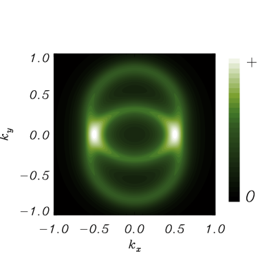
FIG. 1.: Far field intensity Eq. (32) for $A_{0}=0.99$. Space is scaled with diffraction strenght $a_{1}=a_{2}$ and time is scaled with cavity decay $\gamma_{1}=\gamma_{2}$ [33], as reported in Ref.[14, 16]. Other parameters are $\Delta_{1}=\Delta_{2}=-0.25$, $\rho_{1}=0$, $\rho_{2}=1$. The same parameters will be used for all Figures, unless another choice is specified. The lower (upper) ring corresponds to the intensity of the field $1$ ($2$).

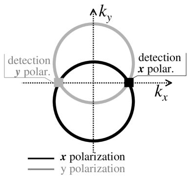
FIG. 2.: FF signal (black) and idler (grey) rings and detection scheme not influenced by the walk-off: The $x$ and $y$ polarizations are detected at the points $\pm\vec{k}_{H}$ where the rings intersect (square symbols).

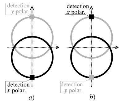
FIG. 3.: FF signal and idler rings and detection scheme influenced by the walk-off: a) The $x$ and $y$ polarized fields are detected in the points $\pm\vec{k}_{V}$ indicated by the square symbols, on the intense $x$ polarized (black) and $y$ polarized (grey) rings (bright detection). b) In the same points $\pm\vec{k}_{V}$ (square symbols) the orthogonal polarizations $y$ and $x$ are detected (dark detection).

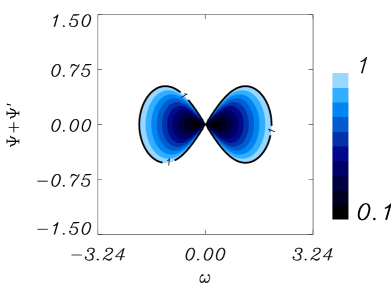
FIG. 4.: ${\mathcal{V}}_{g=1}(\pm\vec{k}_{H},\omega;\vec{\Phi})/{\sigma}$ for $\vec{\Phi}=(\pi,0,\Psi,0,\pi/2,\Psi^{\prime})$ as a function of $\Psi+\Psi^{\prime}$ (rad) and the frequency $\omega$. EPR entanglement is obtained for values less than $1$ (dark line). Values above $1$ outside this line are not displayed.

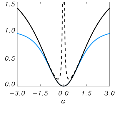
FIG. 5.: ${\mathcal{V}}_{g}(\pm\vec{k}_{H},\omega;\vec{\Phi})/{\sigma}$ for $\Psi+\Psi^{\prime}=0$ and $g=1$ (dark continuous line), for $\Psi+\Psi^{\prime}=0$ and $g=\bar{g}$ (light continuous line), and for $\Psi+\Psi^{\prime}\simeq 0.06$rad and $g=1$ (dashed line).

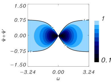
FIG. 6.: Same as in Fig.4, but for the choice $g=\bar{g}$.

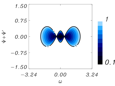
FIG. 7.: ${\mathcal{V}}_{g=1}(\pm\vec{k}_{V},\omega;\vec{\Phi})/{\sigma}$ for $\vec{\Phi}=(\pi,\pi/2,\Psi,0,\pi,\Psi^{\prime})$ as a function of $\Psi+\Psi^{\prime}$ (rad) and the frequency $\omega$. The detection scheme is the one shown in Fig.3a. EPR entanglement is obtained for values less than $1$ (dark line). Values above $1$ outside this line are not displayed.

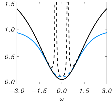
FIG. 8.: Dependence of ${\mathcal{V}}_{g}(\pm\vec{k}_{V},\omega;\vec{\Phi})/{\sigma}$ on the frequency $\omega$, for $\Psi+\Psi^{\prime}=0$ and $g=1$ (dark continuous line), for $\Psi+\Psi^{\prime}=0$ and $g=\bar{g}$ (light continuous line), for $\Psi+\Psi^{\prime}\simeq 0.06$rad and $g=1$ (dark dashed line), and for $\Psi+\Psi^{\prime}\simeq 0.06$rad and $g=\bar{g}$ (light dashed line).

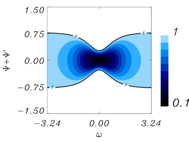
FIG. 9.: ${\mathcal{V}}_{g=\bar{g}}(\pm\vec{k}_{V},\omega;\vec{\Phi})/{\sigma}$ as in Fig.7, but for the choice $g=\bar{g}$.

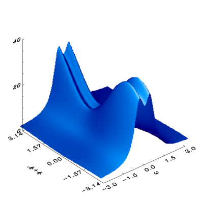
FIG. 10.: ${\mathcal{V}}_{g=1}(\pm\vec{k}_{V},\omega;\vec{\Phi})/{\sigma}$ for $\vec{\Phi}=(\pi,0,\Psi,0,\pi/2,\Psi^{\prime})$, as a function of $\Psi+\Psi^{\prime}$ (rad) and frequency $\omega$. The detection scheme is the one shown in Fig.3b.

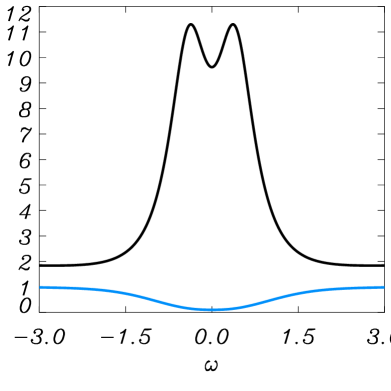
FIG. 11.: Dependence of ${\mathcal{V}}_{g}(\pm\vec{k}_{V},\omega;\vec{\Phi})/{\sigma}$ on the frequency $\omega$, for $\Psi+\Psi^{\prime}=\bar{\Psi}$ and $g=1$ (dark continuous line), for $\Psi+\Psi^{\prime}=\bar{\Psi}$ and $g=\bar{g}$ (light continuous line). $\bar{\Psi}\simeq 0.81$rad.

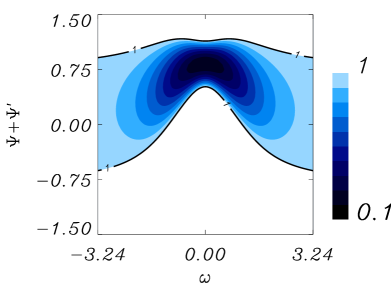
FIG. 12.: Same as in Fig.10, but for the choice of $g=\bar{g}$.EPR entanglement is obtained for values less than $1$ (dark line). Values above $1$ outside this line are not displayed.

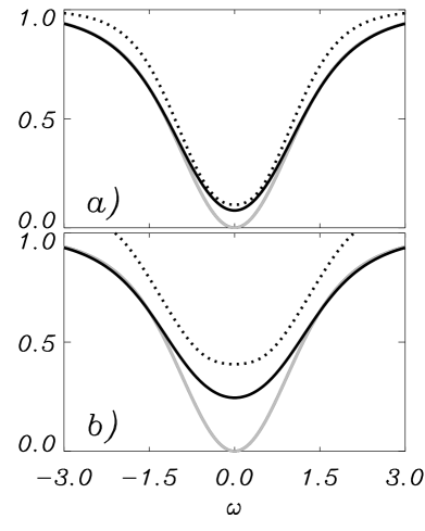
FIG. 13.: Spectral variance ${\mathcal{V}}_{\bar{g}}$ as a function of frequency, for the detection schemes represented in Fig.2 (light line), Fig.3a (dark continuous line), and Fig.3b (dark dotted line). The angles $\Psi+\Psi^{\prime}=0,0,0.81$ rad are selected respectively for each detection scheme. a) walk-off $\rho_{2}=1$; b) walk-off $\rho_{2}=1.5$.

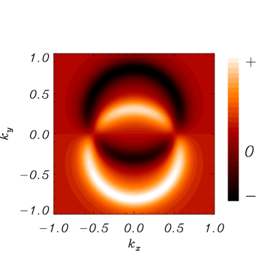
FIG. 14.: Stationary average of the Stokes operator $\langle\hat{S}_{1}(\vec{k})\rangle$ in the FF (Eq.(98)).

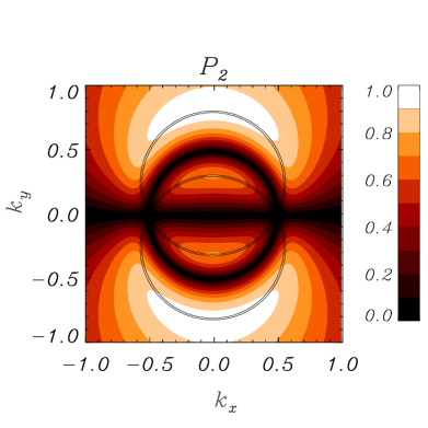
FIG. 15.: Second order polarization degree $P_{2}(\vec{k},t)$ defined in Eq. (100). The two circles of double continuous line show the signal and idler maxima intensities.

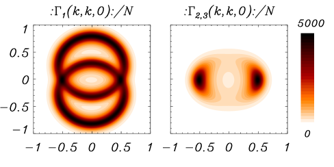
FIG. 16.: Normal ordered variances $\Gamma_{1}(\vec{k},\vec{k},0)$ and $\Gamma_{2,3}(\vec{k},\vec{k},0)$ normalized to the shot noise $N=\langle\hat{S}_{0}(\vec{k},t)\rangle\sigma$.

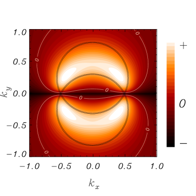
FIG. 17.: $D_{2}(\vec{k},-\vec{k},0)$ normal ordered normalized to the shot noise. The white contour line shows the boundaries between classical and quantum statistics. The two circles of double continuous line show the signal and idler maxima intensities.

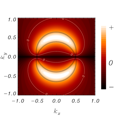
FIG. 18.: The same as in Fig. 17, but with walk-off $\rho_{2}=0.5$.

REFERENCES

- [1] http://www.imedea.uib.es/PhysDept/
- [2] R. Schnabel, W. P. Bowen, N. Treps, T. C. Ralph, H.-A. Bachor, and P. Koy Lam, Phys. Rev. A 67, 012316 (2003), and reference therein.
- [3] Quantum fluctuations and coherence in optical and atomic structures, Special Issue, Eur. Phys. J. D 22, No. 3 (2003) and reference therein.
- [4] P.G. Kwiat, K. Mattle, H. Weinfurter, A. Zeilinger, A. V. Sergienko, and Y.H. Shih, Phys. Rev. Lett. 75, 4337 (1995).
- [5] N. Korolkova, G. Leuchs, R. Loudon, T. C. Ralph, and C. Silberhorn, Phys. Rev. A 65, 052306 (2002).
- [6] W. P. Bowen, N. Treps, R. Schnabel, and P. Koy Lam, Phys. Rev. Lett. 89, 253601 (2002).
- [7] G. Leuchs, Ch. Silberhorn, F. König, A. Sizmann, and N. Korolkova:Quantum solitons in optical fibres: basic requisites for experimental quantum communication, in ”Quantum Information Theory with Continuous Variables”, S.L. Braunstein and A.K. Pati (eds.), Kluwer Academic Publishers, Dodrecht 2002, in press.
- [8] S. Lloyd, S.L. Braunstein, Phys. Rev. Lett. 82, 1784 (1999).
- [9] J. Hald, J. L. Sørensen, C. Schori, and E. S. Polzik, Phys. Rev. Lett. 83, 1319 (1999)
- [10] A. Furusawa et al., Science 282, 706 (1998))
- [11] A. Gatti, R.Zambrini, M. San Miguel and L. A. Lugiato, unpublished.
- [12] Z. Y. Ou and Y. J. Lu, Phys. Rev. Lett. 83, 2556 (1999).
- [13] Oberparleiter, Weinfurter, Opt. Comm. 183, 133 (2000).
- [14] A. Gatti, H. Wiedemann, L. A. Lugiato, I. Marzoli, G. L. Oppo, and S. M. Barnett, Phys. Rev. A 56, 877 (1997).
- [15] C. Szwaj, G.-L. Oppo, A. Gatti, L. A. Lugiato, E. Phys. J. D 10, 433 (2000)
- [16] R. Zambrini, S. M. Barnett, P. Colet, and M. San Miguel, Phys. Rev. A 65, 023813 (2002).
- [17] A. Einstein, B. Podolsky, and N. Rosen, Phys. Rev. 47, 777 (1935).
- [18] Z.Y. Ou, S.F. Pereira, H.J. Kimble, and K.C. Peng, Phys. Rev. Lett. 68, 3663 (1992).
- [19] Y. Zhang, H. Wang, X. Li, J. Jing, C. Xie, and K. Peng, Phys. Rev. A 62, 023813 (2000).
- [20] A. Gatti, L.A. Lugiato, K.I. Petsas and I. Marzoli, Europhys. Lett. 46, 461 (1999).
- [21] A. Gatti, K.I. Petsas, I. Marzoli and L.A. Lugiato Opt. Comm. 179, 591 (2000).
- [22] W. P. Bowen, R. Schnabel, H.-A. Bachor, and P. K. Lam Phys. Rev. Lett. 88, 093601 (2002).
- [23] M.J. Collett and C.W. Gardiner, Phys. Rev. A 30, 1386 (1984).
- [24] For further discussions about singularity problems in presence of a flat pump see Ref. [15].
- [25] G. Izús, M. Santagiustina, M. San Miguel, and P. Colet, J. Opt. Soc. Am. 16, 1592 (1999).
- [26] H. Ward, M. N. Ouarzazi, M. Taki, and P. Glorieux, Phys. Rev. E 63, 016604 (2001).
- [27] C. Jeffries and K. Weisenfeld, Phys. Rev. A 31, 1077 (1985).
- [28] M. D. Reid and P. D. Drummond, Phys. Rev. A 41, 3930 (1990).
- [29] Lu-Ming Duan, G. Giedke, J. I. Cirac, and P. Zoller, Phys. Rev. Lett. 84, 2722 (2000).
- [30] A. S. Chirkin, A. A. Orlov, and D. Y. Paraschuk, Quantum Electron. 23, 870 (1993).
- [31] D. M. Klyshko, JEPT 84, 1065 (1997).
- [32] For further discussions about singularity problems in presence of a flat pump see Ref. [15].
- [33] In this paper we consider the case of symmetrical losses and detunings in the signal, that is a good approximation when there is degeneracy in frequency. The generalization to the case of different losses in a one mode NOPO is considered in: A. S. Lane, M. D. Reid, and D. F. Walls, Phys. Rev. A 38, 788 (1988); G. Björk and Y. Yamamoto, Phys. Rev. A 37, 1991 (1988).
- [34] M. Born and E. Wolf, Principle of Optics (Pergamon, Oxford, 1975).
- [35] E. Hecht, Am. J. of Physics 38, 1156 (1970).
- [36] T. Hakioglu, Phys. Rev. A 59, 1586 (1999).
- [37] T. Tsegaye, J. Söderholm, M. Atatüre, A. Trifonov, G. Björk, A. V. Sergienko, B. E. A. Saleh, and M. C. Teich, Phys. Rev. Lett. 85, 5013 (2000).
- [38] P. Usachev, J. Söderholm, G. Björk, and A. Trifonov, Opt. Commun. 193, 161 (2001).
- [39] J. Söderholm, G. Björk, A. Trifonov, Opt. Spectrosc. 91, 532 (2001).
- [40] H. Prakash and N. Chandra, Phys. Rev. A 4, 796 (1971).
- [41] A. Luis, Phys. Rev. A 66, 013806 (2002)
- [42] J. W. Goodman, Statistical optics (Wiley,New York, 1985), pg. 39.
- [43] These Stokes parameters are function of the discretized FF modes introduced in Eq. 27.
- [44] The factor appears due to the discretization introduced for the fields and is nonvanishing for Stokes parameters measured on overlapping regions.