Abstract

Focusing particularly on one-qubit and two-qubit systems, I explain how the quantum state of a system of $n$ qubits can be expressed as a real function—a generalized Wigner function—on a discrete $2^{n}\times 2^{n}$ phase space. The phase space is based on the finite field having $2^{n}$ elements, and its geometric structure leads naturally to the construction of a complete set of $2^{n}+1$ mutually conjugate bases.

PACS numbers: 03.65.Ca, 03.65.Ta, 03.65.Wj, 02.10.De

On Charlie Bennett’s main webpage one finds two photographs: one of Charlie himself and the other of a vortex created by a beaver dam. A vortex is a wonderful example of a structure that maintains its form by not holding on to its substance; it thrives because it continually gives its material away.

Some summers ago I was supervising four undergraduates in research projects in quantum information theory, and together we drove down to the Watson Research Center for a day to talk with Charlie. He took us to the Croton dam, one of his favorite places. As we sat there on the dam with the sound of water in the background, we discussed quantum information and wrote down quantum states on a large pad of newsprint that Charlie had brought along. The breeze was blowing a bit, and as always around Charlie, ideas were swirling. We talked for hours. In the years that have passed since that afternoon, traces of that experience and traces of those ideas have surely been carried far out into the world—who knows how far—in the lives of those four students and the people they have encountered. I offer this little story as one example of hundreds of similar acts of sharing, through which Charlie Bennett has had an influence on the world of science that could never be captured by any reckoning based on cited publications. It is a pleasure to dedicate this paper to him on the occasion of his sixtieth birthday.

A spin-1/2 particle is probably not a vortex, though there may be some virtue in thinking of it more as a process than a static object. But here I will not be adventurous in that way. This paper is about qubits as normally conceived, and I will use the spin of a spin-1/2 particle as my standard physical example of a qubit. We usually express the quantum state of a system of qubits as a state vector or density matrix. The main point of this paper is to show how one can represent such a quantum state as a real function on a phase space, not a continuous phase space whose axes stand for position and momentum, but a discrete phase space whose axes are associated with a pair of conjugate bases for the finite-dimensional state space. Much of the work I report here was done jointly with Kathleen Gibbons, and many of the mathematical details are given in Ref. [1]. Here I want to lay out the overall contours of this phase space construction.

Discrete phase space representations have been proposed in a number of earlier papers [2–13]. The particular representation to be described here is different in ways that I will discuss later. First, however, I would like to motivate the work by posing what might seem to be an unrelated problem, the problem of determining an unknown quantum state.

1 State determination

Imagine a device whose output is a beam of spin-1/2 particles. We do not know enough about the device to predict the spin state of the particles that it produces. They might all be in the spin-up state, for example, or they might be completely unpolarized. We do, however, assume that the device does not change its operation significantly over time, so that we ought to be able to describe the whole ensemble of particles by a single state (possibly a mixed state) of a single spin-1/2 particle. A general spin state of a spin-1/2 particle can be pictured as a point either on the surface or in the interior of a unit sphere. Points on the surface of the sphere are pure states, points in the interior are mixed states, and the center of the sphere is the completely mixed or completely unpolarized state. Our job is to perform a set of measurements on the particles so as to determine which point represents the spin state actually produced by this mysterious device.

How do we proceed? Suppose we perform the measurement “up vs down” on the first hundred particles that come our way. What do we get from these measurements? We get a rough estimate of the vertical height of the point that represents the ensemble’s state, because the height is what determines the probabilities of “up” and “down”. However we do not get a perfectly precise value of the height, because we have performed only a finite number of trials and therefore still have some statistical error. We know that we will have to live with some statistical error, so we now turn our attention to pinning the state down better along the horizontal dimensions. In order to do this, we perform measurements of spin along two other axes. (Of course we have to use new particles for these measurements. The ones we have already measured hold no further information for us.) If we call the vertical direction $z$, we might let our two new measurements be measurements of spin along the $x$ and $y$ directions. In this way we can narrow the range of likely states to a small region, typically in the interior of the sphere.

It is clear that if we restrict our attention to orthogonal measurements, each represented by a pair of diametrically opposite directions in space, then in order to have any hope of pinning down the state we need to use at least three different measurements. That is, we need to break the whole ensemble into at least three subensembles and measure each of these subensembles along a different axis. As long as the three axes are not coplanar, we will eventually get an arbitrarily good estimate of the state. But some non-coplanar choices are better than others: the statistical error will be minimized if we use three axes that are perpendicular to each other, such as the $x$, $y$, and $z$ axes as imagined above [14]. In this case the three measurements are called “mutually conjugate,” meaning that each eigenvector of one measurement is an equal superposition of the eigenvectors of any of the other measurements. If we choose the measurements in this way, each different measurement gives us information that is as independent as possible of the information provided by the other measurements. A state-determination scheme based on measurements in the $x$, $y$, and $z$ directions is pictured symbolically in Fig. 1, where the measurements are labeled $X$, $Y$, and $Z$.

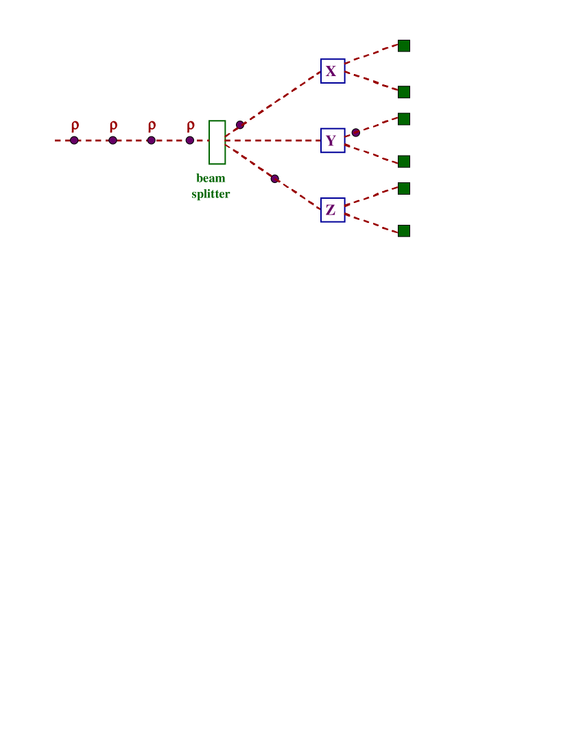
Figure 1: Determining the state of a single qubit. The beam splitter represents the random splitting of the original ensemble into three subensembles.

Let us now consider the problem of state determination for a pair of qubits. We imagine a device that produces a beam of pairs of spin-1/2 particles. For example, each pair might consist of two distinguishable spin-1/2 nuclei in the same molecule. How might we go about determining the state of one of these pairs? One can show that it is sufficient to use the following nine measurements, each performed on a different subensemble [18]: $XX$, $XY$, $XZ$, $YX$, $YY$, $YZ$, $ZX$, $ZY$, $ZZ$. Here $XY$, for example, means measuring the first particle of the pair along the $x$ axis and the second along the $y$ axis. This scheme is illustrated in Fig. 2.

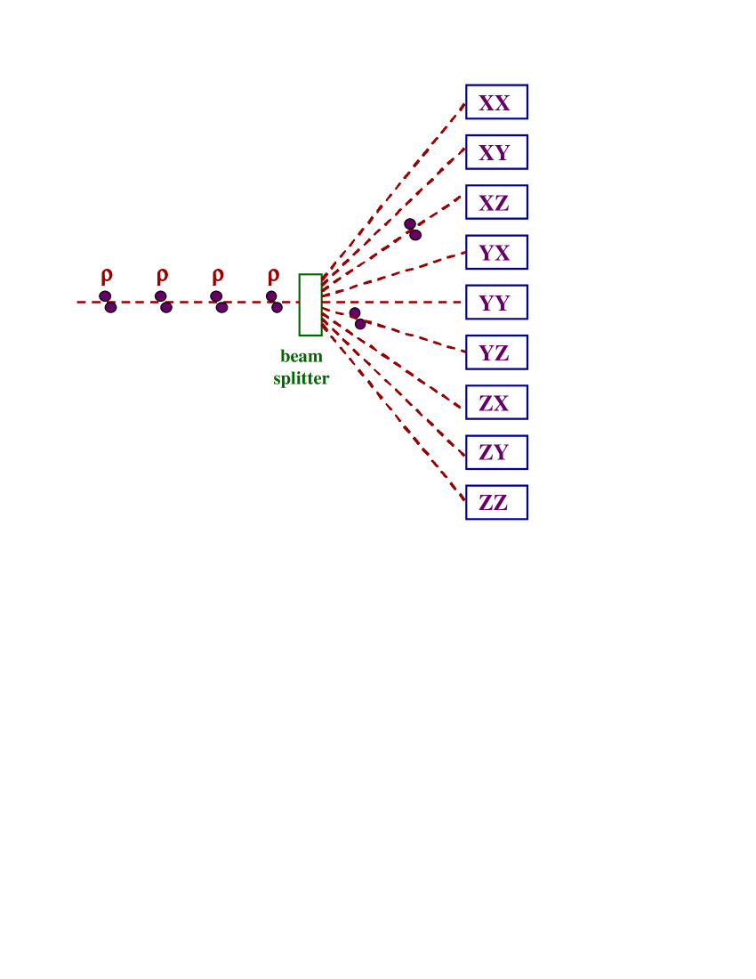
Figure 2: Determining the state of a pair of qubits.

In a certain sense, this nine-measurement scheme is not as efficient as it might be. A general density matrix for a pair of qubits requires $4^{2}-1=15$ real parameters for its specification. A general orthogonal measurement with four outcomes (such as any of the nine measurements listed above) provides $4-1=3$ independent probabilities, since the probabilities must sum to unity. Therefore, if we restrict our attention to orthogonal measurements, we need at least $15/3=5$ such measurements to determine the state. The above scheme thus uses more distinct measurements than would seem to be necessary. We should be able to get away with using only five distinct measurements, and ideally these five measurements would be mutually conjugate so as to minimize the statistical error.

We are thus led to an interesting question: do there exist five orthogonal measurements for a pair of qubits that are all mutually conjugate? The answer is not at all obvious, but it is known: yes, there do exist such measurements [14, 20, 21, 22]. One set that satisfies all the imposed constraints is the following: $XX$, $YY$, $ZZ$, plus two other measurements that are both closely related to the Bell measurement. The Bell measurement, named for John Bell, has the following eigenstates:

$$(1/\sqrt{2})(\mid\uparrow\uparrow\rangle+\mid\downarrow\downarrow\rangle)$$

$$(1/\sqrt{2})(\mid\uparrow\uparrow\rangle-\mid\downarrow\downarrow\rangle)$$

$$(1/\sqrt{2})(\mid\uparrow\downarrow\rangle+\mid\downarrow\uparrow\rangle)$$

$$(1/\sqrt{2})(\mid\uparrow\downarrow\rangle-\mid\downarrow\uparrow\rangle)$$

To get the last two mutually conjugate measurements in our set of five, we rotate the second of the two spins by $120^{\circ}$ around the vector $(1,1,1)$—in one direction or the other—and then perform the Bell measurement. The rotation cyclically permutes the $x$, $y$, and $z$ axes. If the rotation is in the direction $z\rightarrow y\rightarrow x\rightarrow z$, I will call the resulting measurement the “belle” measurement, and if the rotation is in the opposite direction, we get the “beau” measurement. Thus our five mutually conjugate measurements are $XX$, $YY$, $ZZ$, belle, and beau.

Of course one does not have to restrict one’s attention to orthogonal measurements. A single generalized measurement (POVM) with the right number of outcomes, performed on many members of the given ensemble, could be used to determine the state just as efficiently as our conjugate-measurement scheme. I am focusing on the conjugate-measurement scheme mainly because it will lead us to the phase space picture that I want to develop. But in fact mutually conjugate measurements are also interesting in another context, quantum cryptography. From the earliest work on that subject conjugate measurements for qubits have played a special role [24, 25]—Steven Wiesner’s original paper is titled “Conjugate Coding”—and more recently conjugate measurements in higher-dimensional state spaces have likewise been applied to cryptography [26]. They have also been used in a more general analysis of the principle that underlies quantum cryptography, namely, the trade-off between gaining information and preserving the state [27].

It is thus of interest to determine how many mutually conjugate measurements one can find in a general $N$-dimensional state space. The question is really about mutually conjugate bases, since the eigenvalues that one might assign to the outcomes of a measurement are not relevant either for state determination or for cryptography. Two orthonormal bases are mutually conjugate if, given any vector $|v\rangle$ from one of the bases and any vector $|w\rangle$ from another one, the magnitude of the inner product, $|\langle v|w\rangle|$, has a fixed value independent of the choice of vectors—in fact this value must be $1/\sqrt{N}$ in order for the vectors to be normalized. The following facts represent our current state of knowledge about the problem of finding mutually conjugate bases. (1) In a complex vector space of $N$ dimensions, there can exist at most $N+1$ mutually conjugate bases [28, 29]. This is interesting because for state determination, the minimum number of orthogonal measurements needed is also $N+1$, this being the ratio of the number of parameters required to specify a state and the number of independent probabilities one obtains from each measurement: $(N^{2}-1)/(N-1)=N+1$. (2) If $N$ is a power of a prime, then there do exist $N+1$ mutually conjugate bases. Moreover, a number of methods have been devised for constructing such bases in this case [14, 20, 21, 22, 23]. (3) For every $N$ that is not a power of a prime, it is not known whether $N+1$ such bases exist. This is true even for $N=6$.

One interesting feature of the discrete phase space construction described in this paper is that it provides a novel way a generating a complete set of mutually conjugate bases in $N$ dimensions when $N$ is a power of a prime. Before we get to that construction, though, let us review briefly the best known phase-space representation of quantum states of continuous systems, the Wigner function.

2 The Wigner function and quantum tomography

Let $\rho$ be the density matrix of a quantum particle moving in one dimension. The Wigner function $W(q,p)$ is an alternative representation of the quantum state of such a particle [30]. It is defined by

$$W(q,p)=\frac{1}{\pi\hbar}\int\langle q-x|\rho|q+x\rangle\,\exp(2ipx/\hbar)\,dx.$$ (1)

Here $q$ and $p$ are the particle’s position and momentum; so the Wigner function is a real function on ordinary phase space. The integral of the Wigner function over all of phase space is unity, as it would be for a probability distribution, but the Wigner function is not a probability distribution: it can take negative values.

There is, however, an interesting respect in which the Wigner function does act like a probability distribution. Consider any two parallel lines in phase space, described by the equations $aq+bp=c$ and $aq+bp=c^{\prime}$, where $a$, $b$, $c$, and $c^{\prime}$ are real constants. One can show that the integral of the Wigner function over the infinite strip of phase space between these two lines is equal to the probability that the operator $a\hat{q}+b\hat{p}$ will be found to take a value between $c$ and $c^{\prime}$ [5, 31]. In other words, the integral of the Wigner function over any direction in phase space yields the correct probability distribution for an operator associated with that direction. Here a “direction” is defined by a complete set of parallel lines. Such sets of lines will be important for our discrete phase space as well, and we will call them “striations” of the phase space.

The Wigner function has many other special properties [33], of which I will mention just one: translational covariance. Let $\rho$ be an arbitrary state of our one-dimensional particle, and let $W$ be the corresponding Wigner function. The state $\rho^{\prime}$ defined by

$$\rho^{\prime}=\exp[i(q_{0}\hat{p}-p_{0}\hat{q})/\hbar]\,\rho\,\exp[-i(q_{0}\hat{p}-p_{0}\hat{q})/\hbar]$$

represents the result of translating $\rho$ by a displacement $q_{0}$ in space and boosting its momentum by an amount $p_{0}$. When the state is displaced in phase space in this way, the Wigner function follows along as one expects it should: if $W^{\prime}$ is the Wigner function associated with $\rho^{\prime}$, then

$$W^{\prime}(q,p)=W(q-q_{0},p-p_{0}).$$

When we generalize the Wigner function to discrete systems, we will insist on an analog of this translational covariance.

We can use the relation between the Wigner function and actual probability distributions as the basis of a method for determining the quantum state of our one-dimensional particle, assuming that we are given a large ensemble of such particles all described by the same density matrix $\rho$. For each direction in phase space, that is, for each striation, we perform on a subensemble the measurement associated with that striation. Such a measurement can always be represented by an operator of the form $a\hat{q}+b\hat{p}$, and the observed probability distribution for that operator gives us the integral of $W$ along the given direction. From the integrals of $W$ over every direction, it is mathematically possible to reconstruct $W$ itself. The process is closely analogous to medical tomography and is in fact called quantum tomography [31, 32]. Once we have found the Wigner function, we have found the particle’s state, because the Wigner function is an expression of that state. However, if one prefers the density matrix, one can find it via the inverse of Eq. (1):

$$\langle q_{1}|\rho|q_{2}\rangle=\int W\left(\frac{q_{1}+q_{2}}{2},p\right)\,\exp[ip(q_{1}-q_{2})/\hbar]\,dp.$$

Of course in real life we cannot literally perform the infinite number of measurements required by this scheme, but we can estimate the state by performing a large but finite number of measurements.

On first sight quantum tomography may seem impractical because one does not know how to measure a general operator of the form $a\hat{q}+b\hat{p}$. But there is a special case for which such measurements are very natural, namely, the case of a harmonic oscillator. As the quantum state of a harmonic oscillator evolves in time, its Wigner function simply rotates rigidly around the origin of phase space, at least if the relative scale of the position and momentum axes is chosen in the right way. Thus to measure the operator associated with some skew direction, we can simply allow the system to evolve for the right amount of time and then measure the position. Now, a mode of the electromagnetic field can be regarded as a harmonic oscillator. So quantum tomography is particularly suited to finding the quantum state of such a mode, and indeed, quantum tomography has mostly been used in quantum optics.

Notice the similarities between the tomography just described and the method of state determination for one or two qubits described in Section 1. In both cases we use a set of orthogonal measurements which are sufficient for reconstructing all the parameters of the density matrix. If fact, it even turns out that the measurements used in the continuous case are all mutually conjugate: that is, each eigenstate of the operator $a\hat{q}+b\hat{p}$ yields a uniform distribution of the value of $a^{\prime}\hat{q}+b^{\prime}\hat{p}$, as long as $(a,b)$ and $(a^{\prime},b^{\prime})$ define different directions in phase space. The most glaring lack of similarity between the two cases is that in the continuous case the measurements arise naturally from the phase space description of the particle, whereas in the discrete case there is no such description, and the measurements are constructed by other means. The rest of this paper is motivated by the following questions: Can the measurements that we used for determining the state of one or two qubits be obtained from a phase space description of the system? And if so, can this construction be generalized to larger systems? As we will see, the answer to both questions is yes.

3 Phase space for a single qubit

Let us consider first the case of a single qubit, imagined as a single spin-1/2 particle. I will take the horizontal axis of phase space to represent the $z$ component of spin, which takes the two values $\uparrow$ and $\downarrow$. The vertical axis will represent the $x$ component of spin, its two values being $\rightarrow$ and $\leftarrow$. Thus the phase space consists of exactly four points, as shown in Fig. 3a.

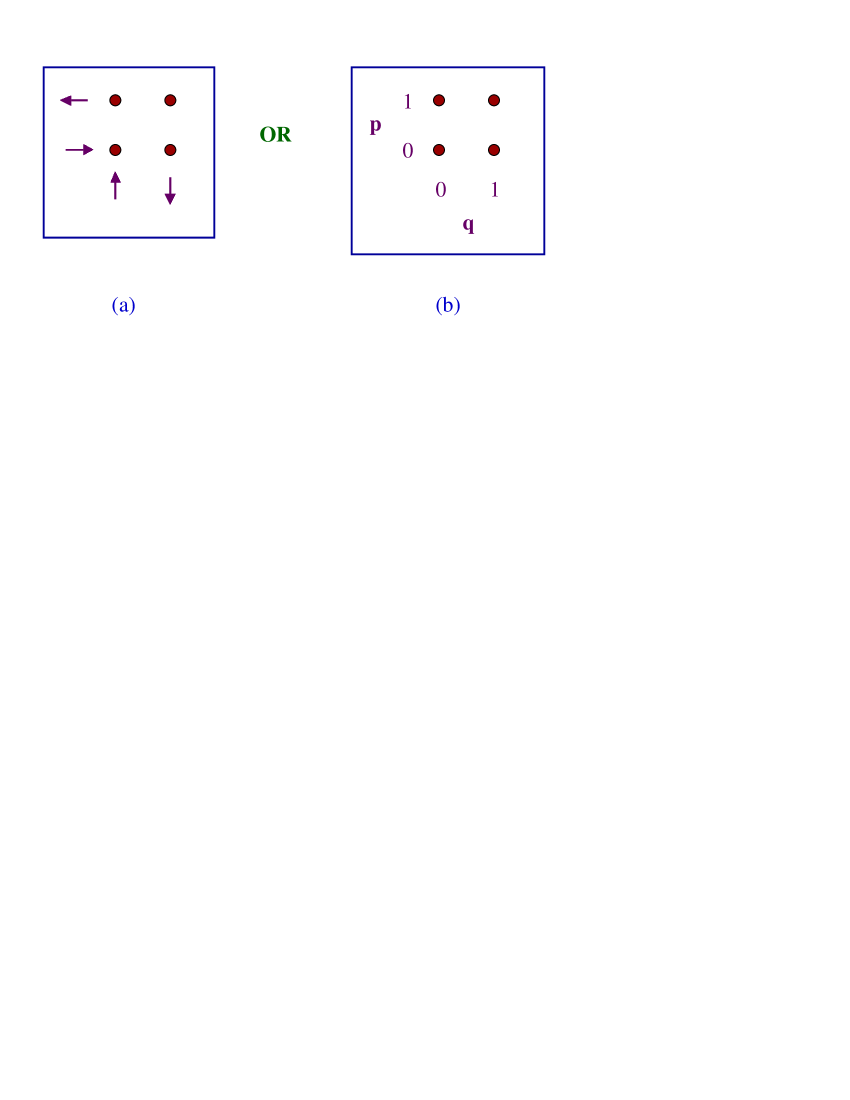
Figure 3: (a) Labeling the phase space with physical states. (b) Labeling the phase space with abstract variables $q$ and $p$ taking values in $\mathbb{Z}_{2}$.

In order to make sense of the notion of a “line” in the discrete phase space, and the notion of “parallel lines,” we want to be able to write down algebraic equations involving the phase space variables. So, in addition to associating with the axes the physical states shown in Fig. 3a, we also want to associate with these axes two variables $q$ and $p$, analogs of position and momentum, that take numerical values. I will let these numerical values be 0 and 1, interpreted as elements of the binary field $\mathbb{Z}_{2}$. That is, addition and multiplication of the values of $q$ and $p$ will be mod 2. This way of labeling the phase space is shown in Fig. 3b.

A line in this phase space is the set of points that satisfies a linear equation, $aq+pb=c$, where $a$, $b$, and $c$ also take values in $\mathbb{Z}_{2}$. For example, the equation $q+p=0$ defines the line consisting of the two points $(0,0)$ and $(1,1)$. It is parallel to the line defined by $q+p=1$, which consists of the points $(0,1)$ and $(1,0)$. In fact there are exactly three sets of parallel lines in this phase space, that is, three striations, and these are shown in Fig. 4.

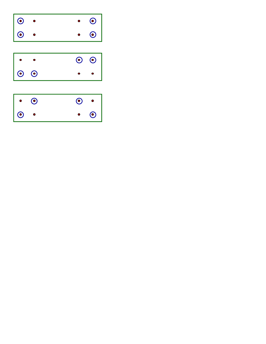
Figure 4: The three striations of the $2\times 2$ phase space.

As in the continuous case, each striation will be associated with a measurement, and each line in the striation will be associated with a particular outcome of the measurement. Shortly we will define a Wigner function on this phase space, which will represent an arbitrary spin state by four real numbers, one for each point in phase space. The Wigner function will have the property that its sum over any line is equal to the probability of the measurement outcome associated with that line.

We are thus led to the following question: What measurement—or more properly, what orthogonal basis—are we to associate with each striation? In labeling the axes, we have implicitly associated bases with the horizontal and vertical striations: the vertical lines are associated with the states $\mid\uparrow\rangle$ and $\mid\downarrow\rangle$, and the horizontal lines are associated with the states $\mid\rightarrow\rangle$ and $\mid\leftarrow\rangle$. So it only remains to associate a basis with the diagonal lines. The reader is likely to be able to guess what basis we will assign to these lines, but I want the structure of the phase space to pick out this basis for us, as if we could not guess it. (The construction will be more impressive in the case of two qubits, where it is harder to guess the measurements.)

The crucial concept for fixing the remaining basis is the concept of a translation in the discrete phase space. A translation is simply the addition, mod 2, of a vector $(q_{0},p_{0})$ to each point in phase space. Note that, according to our physical interpretation of the axes, translating by one unit in the horizontal direction—that is, adding the vector $(1,0)$—amounts to interchanging $\uparrow$ and $\downarrow$ while leaving $\rightarrow$ and $\leftarrow$ unchanged. Physically, these changes correspond to a rotation of the spin by $180^{\circ}$ around the $x$ axis, which is represented mathematically by the unitary operator $\sigma_{x}$, one of the Pauli matrices. We therefore associate a unit horizontal translation on phase space with the operator $\sigma_{x}$ on state space, and we refer to this operator as $H$, the horizontal translation operator. (The operator $\sigma_{x}\exp(i\phi)$, with an arbitrary phase $\phi$, would work just as well. For definiteness we choose $\phi$ to be zero.) Similarly a unit vertical translation must be associated (up to an overall phase factor) with the operator $\sigma_{z}$, which we call $V$. These two unitary operators are analogous to the operators $\exp(iq_{0}\hat{p}/\hbar)$ and $\exp(-ip_{0}\hat{q}/\hbar)$, which effect translations in the continuous phase space.

We will want our Wigner function to be translationally covariant, like the continuous Wigner function. For example, given a Wigner function $W$ that represents some spin state $\rho$, if we change $\rho$ by applying $H$, we want $W$ to change by a horizontal translation; that is, we want the values of $W$ to be swapped in horizontal pairs. In order to achieve covariance for this particular translation, that is, the horizontal translation, we insist that the basis that we associate with the horizontal lines be the basis of eigenvectors of $H$. But these eigenvectors are $\mid\rightarrow\rangle$ and $\mid\leftarrow\rangle$, which, not surprisingly, we have already decided to associate with the horizontal lines. So translational covariance does not tell us anything new about the horizontal lines.

The requirement of translational covariance does give us something new, however, when we apply it to the diagonal lines. In phase space, the diagonal lines are invariant under a combined vertical and horizontal translation. Therefore, the basis we associate with the diagonal lines is the basis of eigenvectors of $VH$. But $VH=\sigma_{z}\sigma_{x}=i\sigma_{y}$, and the eigenvectors of this matrix are the states associated with the spin directions “into the paper” and “out of the paper.” Notice that we would have arrived at these same states if we had multiplied our translation operators in the opposite order: $HV=-i\sigma_{y}$. So these states constitute our third basis, which we associate with the diagonal lines. Thus we started with two conjugate bases, along the $z$ and $x$ directions, and our construction automatically produced a third conjugate basis, along the $y$ direction.

There remains one ambiguity to clear up before we can define the Wigner function for a single qubit. Though our construction with translation operators tells us what basis to associate with the diagonal lines, it does not tell us which basis vector to associate with each line. There are two choices which are equally natural. Let us arbitrarily associate the $+1$ eigenstate of $\sigma_{y}$ with the line $\{(0,0),(1,1)\}$; then the $-1$ eigenstate is associated with the line $\{(0,1),(1,0)\}$. Once this choice is made, the Wigner function of any spin state is determined by the requirement that its sum over any line is equal to probability of the measurement outcome associated with that line. I will not go into the detailed construction here, but will simply give examples of Wigner functions of particular states.

state	Wigner function
$\mid\uparrow\rangle$	$\begin{array}[]{|c|c|}\hline\cr\hbox{\scriptsize$\frac{1}{2}$}&0\\ \hline\cr\hbox{\scriptsize$\frac{1}{2}$}&0\\ \hline\cr\end{array}$
$\mid\rightarrow\rangle$	$\begin{array}[]{|c|c|}\hline\cr 0&0\\ \hline\cr\hbox{\scriptsize$\frac{1}{2}$}&\hbox{\scriptsize$\frac{1}{2}$}\\ \hline\cr\end{array}$
$+1$ eigenstate of $\sigma_{y}$	$\begin{array}[]{|c|c|}\hline\cr 0&\hbox{\scriptsize$\frac{1}{2}$}\\ \hline\cr\hbox{\scriptsize$\frac{1}{2}$}&0\\ \hline\cr\end{array}$
$-1$ eigenstate of $(\sigma_{x}+\sigma_{y}+\sigma_{z})/\sqrt{3}$	$\begin{array}[]{|c|c|}\hline\cr 0.394&0.394\\ \hline\cr-0.183&0.394\\ \hline\cr\end{array}$

The negative number in the last example is the most negative value possible for our one-qubit Wigner function. Note that the sums over lines are legitimate probabilities; for example, in each case the sum of $W$ over the two points $(0,0)$ and $(1,1)$—that is, the lower left and the upper right—is the correct probability of finding the particle with its spin pointing in the positive $y$ direction.

The essential features of this phase-space description of a single spin-1/2 particle were proposed independently by Feynman [4] and Wootters [5] in 1987, and a similar though not identical construction had been worked out a year earlier by Cohen and Scully [3]. So the $2\times 2$ phase space has been around for a while. However, the generalization to two qubits presented in the following section is new.

4 Phase space for a pair of qubits

The state space for a pair of qubits has four dimensions; so I will take the phase space for this system to be a $4\times 4$ array of points. Imagining the qubits as spin-1/2 particles, I will associate the points of the horizontal axis of phase space with the states $\mid\uparrow\uparrow\rangle$, $\mid\uparrow\downarrow\rangle$, $\mid\downarrow\uparrow\rangle$, and $\mid\downarrow\downarrow\rangle$. The vertical axis will represent the conjugate basis consisting of $\mid\rightarrow\rightarrow\rangle$, $\mid\rightarrow\leftarrow\rangle$, $\mid\leftarrow\rightarrow\rangle$, and $\mid\leftarrow\leftarrow\rangle$. This labeling of the axes is shown in Fig. 5a.

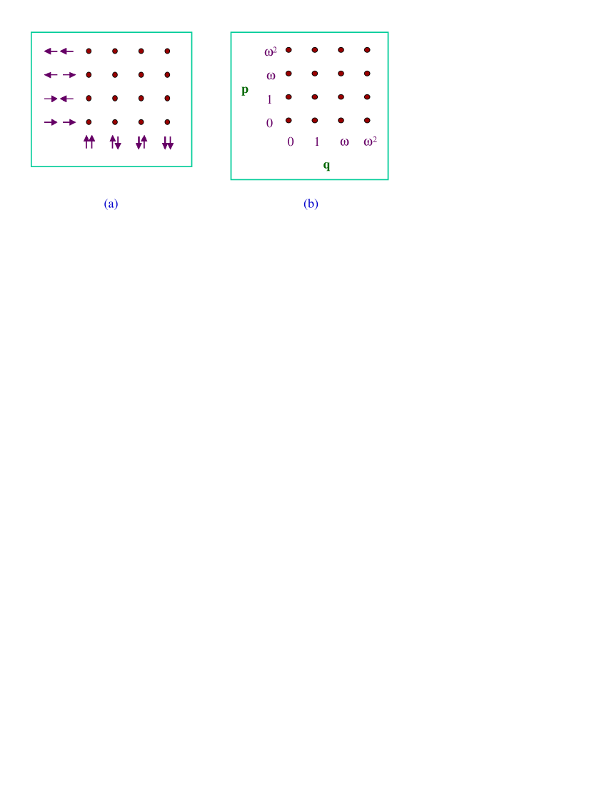
Figure 5: (a) Labeling the $4\times 4$ phase space with physical states. (b) Labeling the same phase space with the variables $q$ and $p$ which take values in $\mathbb{F}_{4}$.

As in the case of a single qubit, we also want to label the axes with variables $q$ and $p$ that take numerical values. The choice of the numerical values is perhaps the most novel feature presented in this paper: $q$ and $p$ will take values in the four-element field $\mathbb{F}_{4}$, whose elements I will write as $\{0,1,\omega,\omega^{2}\}$. We thus get the labeling shown in Fig. 3b. The arithmetic of $\mathbb{F}_{4}$ is the only commutative, associative, and distributive arithmetic on four elements in which both addition and multiplication have inverses [34]. This arithmetic is defined by the following relations:

$$1+1=\omega+\omega=\omega^{2}+\omega^{2}=0$$

$$1+\omega=\omega^{2}$$

$$(\omega)(\omega^{2})=1$$

Notice that it is not the same as arithmetic mod 4. In arithmetic mod 4 there is no multiplicative inverse, because there is no number by which we can multiply 2 to get 1.

The arithmetic of the four-element field actually makes some physical sense for our pair of spin-1/2 particles. Consider, for example, a horizontal translation by the field element 1. This translation interchanges the first two columns ($0\leftrightarrow 1$) as well as the last two columns ($\omega\leftrightarrow\omega^{2}$). According to the labeling given in Fig. 3, this permutation corresponds to interchanging $\uparrow$ and $\downarrow$ for the second particle (while keeping $\rightarrow$ and $\leftarrow$ unchanged), and leaving the first particle entirely unaffected. Physically this corresponds to rotating the second particle by $180^{\circ}$ around the $x$ axis. All the other translations on this phase space, defined by adding other vectors under the addition rules of $\mathbb{F}_{4}$, similarly have simple physical interpretations. From these interpretations we can directly write down unitary translation operators corresponding to the phase-space translations. For example, the translation mentioned above—a horizontal translation by the field element 1—is associated with the unitary operator $I\otimes\sigma_{x}$. We call this operator $H_{1}$, the subscript indicating the field element by which we are translating. For this two-qubit case there are four basic translation operators, which I list here.

$$H_{1}=I\otimes\sigma_{x}$$

$$H_{\omega}=\sigma_{x}\otimes I$$ (2)

$$V_{1}=I\otimes\sigma_{z}$$

$$V_{\omega}=\sigma_{z}\otimes I$$

All other translations can be obtained as combinations of these four. For example, translating by the vector $(1,\omega^{2})$ can be decomposed into a horizontal translation by 1, a vertical translation by $\omega$, and a vertical translation by 1 (since $\omega^{2}=1+\omega$). This translation is therefore associated with the unitary operator $H_{1}V_{\omega}V_{1}=-i\sigma_{z}\otimes\sigma_{y}$. (As before, the order of multiplication of the $H$’s and $V$’s only affects the overall phase factor, which will not be significant for any of what follows.)

As in the case of a single qubit, the notion of a striation is crucial to our construction. Again, lines are defined as the solutions to linear equations, and two lines are parallel if they can be represented by equations that differ only in the constant term. One finds that in the two-qubit phase space there are exactly five striations, which are shown in Fig. 6. Though the lines may not look like lines, notice that the usual rules about parallel lines in a plane hold in this space as well: if two lines are parallel, they have no point in common, and if two lines are not parallel, they have exactly one point in common. These rules follow from the fact that arithmetic in a field is so well behaved, particularly that multiplication is invertible. If we had defined our lines on the basis of mod 4 arithmetic—this arithmetic produces “wrap-around lines”—it would have been possible for two distinct lines to have two points in common.

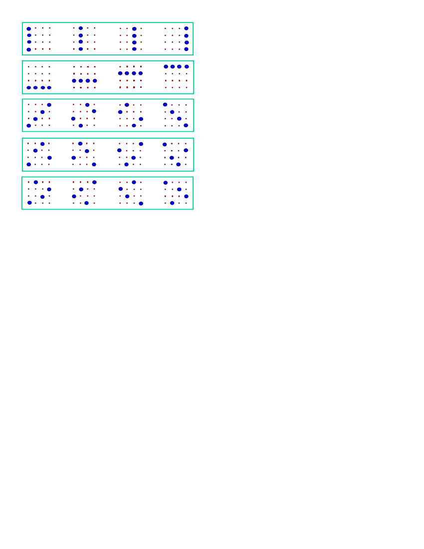
Figure 6: The five striations of the $4\times 4$ phase space.

In order to define a Wigner function, we need to associate an orthogonal basis with each striation. To see how this association is done, let us consider as an example the fourth striation listed in Fig. 6. Notice that each line of this striation is invariant under translations by the vectors $(1,\omega)$, $(\omega,\omega^{2})$, and $(\omega^{2},1)$. These translations are associated with the unitary operators $H_{1}V_{\omega}$, $H_{\omega}V_{\omega}V_{1}$, and $H_{\omega}H_{1}V_{1}$, respectively. Therefore, we want the basis vectors that we assign to these lines to be eigenvectors of all three operators, if that is possible. One can check that these three operators commute with each other; so it is indeed possible to find simultaneous eigenvectors. Moreover this criterion picks out a unique basis, which I write out here in the standard representation in which $\sigma_{z}=\left(\begin{array}[]{cc}1&0\\ 0&-1\end{array}\right)$ and $\sigma_{x}=\left(\begin{array}[]{cc}0&1\\ 1&0\end{array}\right)$.

$$\frac{1}{2}\left(\begin{array}[]{c}1\\ 1\\ i\\ -i\end{array}\right)\hskip 17.07164pt\frac{1}{2}\left(\begin{array}[]{c}1\\ 1\\ -i\\ i\end{array}\right)\hskip 17.07164pt\frac{1}{2}\left(\begin{array}[]{c}1\\ -1\\ i\\ i\end{array}\right)\hskip 17.07164pt\frac{1}{2}\left(\begin{array}[]{c}1\\ -1\\ -i\\ -i\end{array}\right)$$ (3)

One can verify that this is the “belle” basis described in Section 1. In the same way, one finds that the bases associated with the other four striations are precisely the other mutually conjugate bases listed in Section 1. In the order in which the striations are listed in Fig. 6, the corresponding bases are $ZZ$, $XX$, $YY$, belle, and beau. So the measurements we imagined using for state determination do come from a phase space, just as they do in the continuous case.

Let us recapitulate the steps by which we obtain an orthogonal basis from each striation. (1) Two conjugate bases are chosen at the beginning to be associated with the vertical and horizontal striations. (2) From this assignment, one derives a set of unitary operators on state space that correspond to the translations of phase space. (3) Each striation defines a set of phase-space translations that preserve the lines of that striation. (4) The simultaneous eigenvectors of the corresponding unitary operators constitute the basis that we associate with the given striation.

This procedure raises a number of questions, mostly having to do with its potential generalization to other dimensions. Will it always happen that all the translation operators associated with a given striation commute with each other? Will the number of striations always be equal to the number of orthogonal measurements one needs for state determination? And if every striation does generate a definite orthogonal basis, are the bases associated with different striations guaranteed to be conjugate? I will address these questions in the following section. For now, I would like to return to the definition of the Wigner function for a pair of qubits.

Even though we now have a definite correspondence between striations of the phase space and bases for the state space, we have not yet specified which vector in each basis goes with each line of the corresponding striation. As in the single-qubit case, there is no unique way of choosing this assignment. However, the choices are not completely arbitrary. Consider, for example, the first line of the fourth striation shown in Fig. 6. It consists of the points $(0,0)$, $(1,\omega)$, $(\omega,\omega^{2})$, and $(\omega^{2},1)$. To this line, we can assign any of the four “belle” basis vectors listed in Eq. (3). But once we choose one of these vectors, there is no further choice involving that particular striation and that particular basis. This is because the other lines of that striation can be obtained by translating the first one. We can therefore use the following rule: if line $\lambda_{2}$ is obtained from line $\lambda_{1}$ by a translation $T$, then the basis vector we assign to $\lambda_{2}$ should be obtained from the basis vector assigned to $\lambda_{1}$ by the unitary operator associated with $T$. Indeed, one can show that this rule must be followed if the resulting Wigner function is to be translationally covariant [1]. So overall, there is some arbitrariness in the assignment of basis vectors to lines, but not as much arbitrariness as one might have expected.

Once every line in phase space has been assigned a state vector from the appropriate basis, the definition of the Wigner function $W$ is determined: it is determined by the requirement that the sum of $W$ over any line in phase space is equal to the probability of the measurement outcome associated with that line. In order to get a definite Wigner function, I will choose the following correspondence between lines and state vectors.

line		state
$\begin{array}[]{cccc}\circ&\circ&\circ&\bullet\\ \circ&\circ&\bullet&\circ\\ \circ&\bullet&\circ&\circ\\ \bullet&\circ&\circ&\circ\end{array}$	$\longleftrightarrow$	$\frac{1}{2}\left(\begin{array}[]{c}1\\ -i\\ i\\ 1\end{array}\right)$
$\begin{array}[]{cccc}\circ&\circ&\bullet&\circ\\ \circ&\bullet&\circ&\circ\\ \circ&\circ&\circ&\bullet\\ \bullet&\circ&\circ&\circ\end{array}$	$\longleftrightarrow$	$\frac{1}{2}\left(\begin{array}[]{c}1\\ 1\\ i\\ -i\end{array}\right)$
$\begin{array}[]{cccc}\circ&\bullet&\circ&\circ\\ \circ&\circ&\circ&\bullet\\ \circ&\circ&\bullet&\circ\\ \bullet&\circ&\circ&\circ\end{array}$	$\longleftrightarrow$	$\frac{1}{2}\left(\begin{array}[]{c}1\\ -i\\ 1\\ i\end{array}\right)$

These three choices fix the assignments of vectors to lines for the last three bases—$YY$, belle, and beau—and therefore fix the definition of the Wigner function.

With these choices, the Wigner function can be worked out for any two-qubit state [1], some examples of which are shown below.

state	Wigner function
$\mid\uparrow\uparrow\rangle$	$\begin{array}[]{|c|c|c|c|}\hline\cr\hbox{\scriptsize$\frac{1}{4}$}&0&0&0\\ \hline\cr\hbox{\scriptsize$\frac{1}{4}$}&0&0&0\\ \hline\cr\hbox{\scriptsize$\frac{1}{4}$}&0&0&0\\ \hline\cr\hbox{\scriptsize$\frac{1}{4}$}&0&0&0\\ \hline\cr\end{array}$
$\mid\uparrow\rightarrow\rangle$	$\begin{array}[]{|c|c|c|c|}\hline\cr 0&0&0&0\\ \hline\cr\hbox{\scriptsize$\frac{1}{4}$}&\hbox{\scriptsize$\frac{1}{4}$}&0&0\\ \hline\cr 0&0&0&0\\ \hline\cr\hbox{\scriptsize$\frac{1}{4}$}&\hbox{\scriptsize$\frac{1}{4}$}&0&0\\ \hline\cr\end{array}$
$\frac{1}{\sqrt{2}}(\mid\uparrow\downarrow\rangle-\mid\downarrow\uparrow\rangle)$	$\begin{array}[]{|c|c|c|c|}\hline\cr 0&0&0&0\\ \hline\cr 0&\hbox{\scriptsize$\frac{1}{4}$}&\hbox{\scriptsize$\frac{1}{4}$}&0\\ \hline\cr 0&\hbox{\scriptsize$\frac{1}{4}$}&\hbox{\scriptsize$\frac{1}{4}$}&0\\ \hline\cr 0&0&0&0\\ \hline\cr\end{array}$

Again one can check that the sums over lines make sense. For example, the sum over the first vertical line in each case is the probability of finding the pair in the state $\mid\uparrow\uparrow\rangle$.

To return to the problem of state determination, we see that tomography for a two-qubit system is very similar to tomography for a continuous system. Each “direction” in phase space, as defined by a striation, is associated with a measurement, and the collection of measurements obtained in this way is just sufficient to determine the state of the system. It is interesting that, in a paper on reconstructing the state of discrete quantum systems, Asplund and Björk discuss the use of mutually conjugate bases and refer to these bases as being like different directions in phase space [35]. The above construction based on the four-element field shows, at least for two qubits, that this analogy is indeed quite apt.

5 Generalization to other dimensions

To what extent can the above phase-space representations be generalized to state spaces of other dimensions? First, it is crucial to our construction that the axes be labeled by the elements of a field, with its invertible addition and multiplication. Now, it is a fact that there exists a field with $N$ elements if and only if $N$ is a power of a prime, and in that case, there is essentially only one field possible [34]. So our construction does not apply directly to every quantum system, but it does apply to a system of $n$ qubits, since the dimension then is $N=2^{n}$, which is a power of a prime. When the phase space axes are labeled by the $N$-element field, it is not hard to show that the number of striations is $N+1$, exactly the number of orthogonal bases needed for state determination.

Moreover, whenever the dimension is a power of a prime, it turns out that there is a systematic way of labeling the axes with field elements so that the above construction always works. That is, the translation operators associated with a given striation commute with each other and define a unique basis of eigenstates, and the bases thereby derived are guaranteed to be mutually conjugate [1]. Thus this phase-space construction provides a new method of generating a complete set of mutually conjugate bases whenever the dimension $N$ is a power of a prime. It is closely related to, and indeed is inspired by, the methods of Bandyopadhyay et al [21] and Lawrence et al [22]. For example, our translation operators appear in these earlier constructions, though not as translation operators per se. Our method is distinguished from these others in that it is based on phase space and is explicitly geometrical.

6 Discussion

The phase-space representation presented in this paper follows many other papers on discrete phase spaces. As I have said earlier, Feynman proposed the $2\times 2$ phase space we are using for a single spin-1/2 particle [4]. He was interested in the concept of negative probability and asked whether some or all of the mysteries of quantum mechanics could be rendered more intelligible if we could make sense of negative probabilities. Discrete phase spaces for higher-dimensional quantum systems have been proposed by a number of authors. In the formulations of Cohendet et al [6], Galetti and de Toledo Piza [7], Leonhardt [9], and Wootters [5], one sees manifestations of certain number-theoretic issues that arise when one tries to generalize the Wigner function to discrete systems. The work of Cohendet et al, for example, applies only to systems with an odd-dimensional state space. My own earlier work, as well as that of Galetti and de Toledo Piza, applies most naturally to systems for which the dimension $N$ of the state space is prime, though one can also apply it to any composite value of $N$ by treating each prime factor separately. Leonhardt, who introduced a systematic, phase-space approach to finite-state tomography, finds problems with even-dimensional state spaces that he avoids by making his discrete phase space a $2N\times 2N$ grid when $N$ is even. Other approaches use an $N\times N$ phase space for arbitrary $N$ but do not insist on any special properties associated with striations other than those defined by the two axes [10, 12]. A discrete Wigner function adapted particularly to quantum optics was introduced by Vaccaro and Pegg [8] (see also the review by Miranowicz et al [36]), and a Wigner function applicable whenever the configuration space is a finite group of odd order has been developed by Mukunda et al [13]. Recently various authors have used both the Wigner function of Ref. [5] for prime $N$ [37], and Leonhardt’s $2N\times 2N$ formulation generalized to all $N$ [11], to analyze quantum information processes such as Grover’s search algorithm and teleportation.

The work I have described here follows most naturally from Ref. [5] and is essentially a generalization of that paper from the primes to the powers of primes. This new work is also more systematic than Ref. [5] in that it brings out the choices one needs to make in defining a discrete Wigner function. Further details about these choices, and about how many truly distinct definitions are possible, are spelled out in Ref. [1].

As the authors of Refs. [37] and [11] have already shown, there is some value in using phase space to visualize the effects of quantum information processing. I am hoping that the Wigner function described here will have its own advantages in this respect. Another possible application is in the foundations of quantum mechanics. Hardy [38] and Spekkens [39] have recently proposed toy models of quantum mechanics that facilitate the study of certain foundational issues. Our discrete Wigner function appears to provide a natural framework in which to express these toy models and relate them to standard quantum mechanics. For example, in both Hardy’s and Spekkens’ models, a “toybit” has exactly four underlying ontic states, which could be taken to correspond to the four points of our one-qubit phase space. Moreover these models allow exactly six pure epistemic states, which correspond to the six one-qubit Wigner functions in which two of the four values are zero and the other two are 1/2.

For many purposes, it is good to have a way of picturing quantum states. Discrete Wigner functions allow such picturing in that they require us to imagine only three dimensions: two for phase space itself and one for the value of $W$. I have to admit that as a picture, a discrete Wigner function will never be as graceful as, say, a Bennett photograph, but it may give us a new perspective on some of the remarkable things that Charlie and others have shown can be done with qubits.

References

- [1] K. S. Gibbons and W. K. Wootters, “Discrete Phase Space Based on Finite Fields,” in preparation.
- [2] Discrete phase space descriptions have arisen naturally from the study of quantum systems with an imposed periodicity. Papers exemplifying this line of research are J. Schwinger, Proc. Nat. Acad. Sci 46, 570 (1960); F. A. Buot, Phys. Rev. B 10, 3700 (1974); J. H. Hannay and M. V. Berry, Physica D 1, 267 (1980); P. Kasperkovitz and M. Peev, Annals of Physics 230, 21 (1994); A. Bouzouina and S. De Bièvre, Comm. Math. Phys. 178, 83 (1996); A. M. F. Rivas and A. M. Ozorio de Almeida, Annals of Physics 276, 123 (1999).
- [3] L. Cohen and M. Scully, Found. Phys. 16, 295 (1986).
- [4] R. Feynman, “Negative Probabilities” in Quantum Implications: Essays in Honour of David Bohm, edited by B. Hiley and D. Peat (Routledge, London, 1987).
- [5] W. K. Wootters, Annals of Physics 176, 1 (1987).
- [6] O. Cohendet, Ph. Combe, M. Sirugue, and M. Sirugue-Collin, J. Phys. A 21, 2875 (1988).
- [7] D. Galetti and A. F. R. De Toledo Piza, Physica A 149, 267 (1988).
- [8] J. A. Vaccaro and D. T. Pegg, Phys. Rev. A 41, 5156 (1990).
- [9] U. Leonhardt, Phys. Rev. Lett. 74, 4101 (1995); Phys. Rev. A 53, 2998 (1996); Phys. Rev. Lett. 76, 4293 (1996).
- [10] A. Luis and J Peřina, J. Phys. A 31, 1423 (1998).
- [11] P. Bianucci, C. Miquel, J. P. Paz, and M. Saraceno, quant-ph/0106091; C. Miquel, J. P. Paz, M. Saraceno, E. Knill, R. Laflamme, and C. Negrevergne, quant-ph/0109072; C. Miquel, J. P. Paz, M. Saraceno, Phys. Rev. A 65, 062309 (2002); J. P. Paz, Phys. Rev. A 65, 062311 (2002).
- [12] A. Takami, T. Hashimoto, M. Horibe, and A. Hayashi, quant-ph/0010002; see also M. Horibe, A. Takami, T. Hashimoto, and A. Hayashi, quant-ph/0108050.
- [13] N. Mukunda, S. Chaturvedi, and R. Simon, quant-ph/0305127.
- [14] W. K. Wootters and B. D. Fields, Annals of Physics 191, 363 (1989).
- [15] D. G. Fischer, S. H. Kienle, and M. Freyberger, Phys. Rev. A 61, 032306 (2000).
- [16] R. Derka, V. Bužek, and A. K. Ekert, Phys. Rev. Lett. 80, 1571 (1998).
- [17] V. Bužek, G. Drobny, R. Derka, G. Adam, and H. Wiedermann, quant-ph/9805020.
- [18] S. Bergia, F. Cannata, A. Cornia, and R. Livi, Found. Phys. 10, 723 (1980); W. K. Wootters, in Complexity, Entropy, and the Physics of Information, edited by W. H. Zurek (Addison-Wesley, New York, 1991), pp. 39-46.
- [19] G. M. D’Ariano, L. Maccone, and M. Paini, J. Opt. B: Quantum Semiclass. Opt. 5, 77 (2003).
- [20] A. R. Calderbank, P. J. Cameron, W. M. Kantor, and J. J. Seidel, Proc. London Math. Soc. 75, 436 (1997).
- [21] S. Bandyopadhyay, P. O. Boykin, V. Roychowdhury, and F. Vatan, quant-ph/0103162. See also A. Yu. Vlasov, quant-ph/0302064.
- [22] J. Lawrence, C. Brukner, A. Zeilinger, Phys. Rev. A 65, 032320 (2002).
- [23] S. Chaturvedi, Phys. Rev. A 65, 044301 (2002).
- [24] S. Wiesner, Sigact News, 15, no. 1, 78 (1983).
- [25] C. H. Bennett and G. Brassard, in Proceedings of the IEEE International Conference on Computers, Systems, and Signal Processing, Bangalore, India (IEEE, New York, 1984), pp. 175-179.
- [26] H. Bechmann-Pasquinucci and A. Peres, Phys. Rev. Lett. 85, 3313 (2000); D. Bruß and C. Machiavello, Phys. Rev. Lett. 88, 127901 (2002); N. J. Cerf, M. Bourennane, A. Karlsson, and N. Gisin, Phys. Rev. Lett. 88, 127902 (2002); D. B. Horoshko and S. Ya. Kilin, quant-ph/0203095; P. O. Boykin, quant-ph/0210194.
- [27] H. Barnum, quant-ph/0205155.
- [28] P. Delsarte, J. M. Goethals, and J. J. Seidel, Philips Res. Repts. 30, 91 (1975).
- [29] I. D. Ivanovic, J. Phys. A 14, 3241 (1981).
- [30] E. P. Wigner Phys. Rev. 40, 749 (1932).
- [31] J. Bertrand and P. Bertrand, Foundations of Physics 17, 397 (1987); K. Vogel and H. Risken, Phys. Rev. A 40, 2847 (1989); D. T. Smithey, M. Beck, M. G. Raymer, and A. Faridani, Phys. Rev. Lett. 70, 1244 (1993).
- [32] For a review, see U. Leonhardt, Measuring the Quantum State of Light (Oxford Univ. Press, Oxford, 1997).
- [33] M. Hillery, R. F. O’Connell, M. O. Scully, and E. P. Wigner Phys. Rep. 106, 123 (1984).
- [34] R. Lidl and H. Niederreiter, Introduction to finite fields and their applications (Cambridge Univ. Press, Cambridge 1986).
- [35] R. Asplund and G. Björk, Phys. Rev. A 64, 012106 (2001).
- [36] A. Miranowicz, W. Leonski, and N. Imoto, Adv. Chem. Phys. 119, 155 (2001).
- [37] M. Koniorczyk, V. Bužek, and J. Janszky, Phys. Rev. A 64, 034301 (2001).
- [38] L. Hardy, quant-ph/9910028.
- [39] R. Spekkens, “In defense of the epistemic view of quantum states,” lecture available at http://perimeterinstitute.ca/activities/seminarseries/ alltalks.cfm.