Multi-photon, multi-mode polarization entanglement in parametric down-conversion

Abstract

We study the quantum properties of the polarization of the light produced in type II spontaneous parametric down-conversion in the framework of a multi-mode model valid in any gain regime. We show that the the microscopic polarization entanglement of photon pairs survives in the high gain regime (multi-photon regime), in the form of nonclassical correlation of all the Stokes operators describing polarization degrees of freedom.

I Introduction

The quantum properties of light polarization have been widely studied in the regime of single photon counts. In comparison, only recently there has been a rise of interest towards the quantum properties of the polarization of macroscopic light beams Bowen ; Korolkova ; Bowen2 ; Bowen3 , mainly due to their potential applications to the field of quantum information with continuous variables and to the possibility of mapping the quantum state from light to atomic media Polzik .
A well-known source of polarization entangled photons is parametric down-conversion in a type II crystal. Here, a pump field at high frequency is partially converted into two fields at lower frequency, distinguished by their polarizations. Due to spatial walk-off in the crystal, the two emission cones are slightly displaced one with respect to the other, and the the far-field intensity distribution has the shape of two rings, whose centers are displaced along the walk-off direction, as e.g. shown by Fig.1.

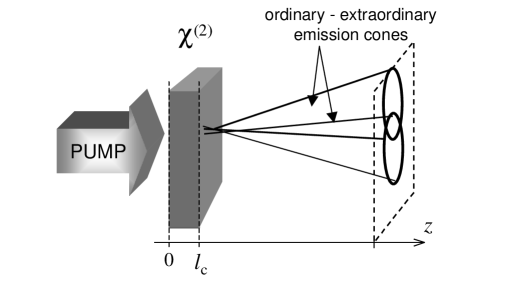
Figure 1: Parametric down-conversion from a type II crystal showing the two down-conversion cones at degeneracy.

The two regions where the far-field rings intersect have a very special role. In the regime of single photon pair detection, the polarization of a photon detected in one of this region is completely undetermined. However, once the polarization of one photon has been measured, the polarization of the other photon, which propagates at the symmetric position, is exactly determined. In other words, when considering photodetection from these regions, the two-photon state can be described as the ideal polarization-entangled statekwiat . Photons produced by this process has become an essential ingredient in many implementations of quantum imformation schemes (see e.g. teleportation ; cryptography ).

The question that we address in this paper is whether the microscopic photon polarization entaglement leaves any trace in the regime of high parametric down-conversion efficiency, where the number of down-converted photons can be rather large Ottavia , and in which form.

To this end parametric down-conversion is described in the framework of a multi-mode model, valid for any gain regime, which includes typical effects present in a realistic crystal, as diffraction and spatio-temporal walk-off. Quantum-optical polarization properties of the down-converted light are described within the formalism of Stokes operators. These operators obey to angular momentum-like commutation rules, and the associated observables are in general non compatible. We define a local version of Stokes operators and study the quantum correlation between Stokes operators measured from symmetric portions of the beam cross-section in the far field zone. In the regions where the two down-conversion cones intersect we find that all the Stokes operators are correlated at the quantum level. Although the light is completely unpolarized and Stokes operators are very noisy, a measurement of a Stokes parameter in one of these regions in any polarization basis determines the value of the Stokes parameter in the symmetric region within an uncertainty much below the standard quantum limit.

A continuous variable polarization entanglement, in the form of quantum correlation between Stokes operators of two light beams, have been recently demonstrated Bowen2 . In this work the entanglement is of macroscopic nature, and spatial degrees of freedom do not play any role since the beams are single-mode. Continuous variable polarization entanglement which takes into account spatial spatial degrees of freedom of light beams is described in Zambrini , where we study the properties of the light emitted by a type II optical parametric oscillator below threshold.
The analysis of this paper is rather focussed on providing a bridge between the miscroscopic and macroscopic domain, since our model is able to describe the polarization entanglement in parametric down-conversion with a continuous passage from the single photon pair production regime to the regime of high down-conversion efficiency.
Besides its fundamental interest, we believe that the form of entanglement described in this work can be quite promising for new quantum information schemes, due the increased number of degrees of freedom in play (photon number, polarization, frequency and spatial degrees of freedom), and is well inserted in the recent trend toward entangled state of increasing complexity (see e.g. Bowmeester , where a four-photon polarization entangled state is characterized)

The paper is organised as follow. Section II describes the model for spontaneous parametric down-conversion, in terms of propagation equations for field operators. Similar models are known in literature (see e.g. Misharev and references quoted therein), but besides presenting it in a systematic way, we include all the relevant features of propagation through a nonlinear crystal and we provide a precise link with the empirical parameters of real crystals. Section III is devoted to the description of the quantum polarization properties of the down-converted light. Stokes operators definition and properties are briefly reviewed in section III.1. In Sec III.2 we generalize this definition to a local measurement in the beam far field plane, and we introduce the spatial correlation functions of interest. Analytical and numerical results for the degree of correlation of the various Stokes parameters detected from symmetric portions of the beam cross-section are presented in sections III.3, III.4, both in the case when a narrow frequency filter is employed (Sec.III.4.1), and when the filter is broad-band (Sec.III.4.2). Section IV provides an alternative description of the system and of its polarization correlations in the framework of the quantum state formalism. Section V finally concludes.

II A multi mode model for type II parametric down-conversion

II.1 Field propagation

The starting point of our analysis is an equation describing the propagation of the three waves (signal, idler and pump) inside a nonlinear $\chi^{(2)}$ crystal. We consider a crystal slab of length $l_{c}$, ideally infinite in the transverse directions, cut for type II quasi-collinear phase-matching. In the framework of the slowly varying envelope approximation the electric field operator associated to the three waves is described by means of three quasi-monochromatic wave-packets. We take the $z$ axis as the laser pump mean propagation direction (Fig.1), and indicate with $\vec{x}=(x,y)$ the position coordinates in a generic transverse plane. $\hat{E}^{(+)}_{i}(z,\vec{x},t)$, $i=o,e,p$ designate the positive frequency part of the field operator (with dimensions of a photon annihilation operator) associated to the ordinary ($i=o$, the ”signal”) and extraordinary ($i=e$, the ”idler”) polarization components of the downconverted beam, and ($i=p$ the ”pump”) the high frequency laser beam activating the down-conversion process. Next we introduce their Fourier transform in time and in the transverse domain:

$$\hat{A}_{i}(z,\vec{q},\Omega)=\int\frac{{\rm d}\vec{x}}{2\pi}\int\frac{{\rm d}t}{\sqrt{2\pi}}{\rm e}^{-{\rm i}\vec{q}\cdot\vec{x}}{\rm e}^{{\rm i}(\omega_{i}+\Omega)t}\hat{E}^{(+)}_{i}(z,\vec{x},t)\qquad i=o,e,p$$ (1)

Here $\vec{q}$ is the transverse component of the wave-vector and $\Omega$ represents the frequency offset from the carriers $\omega_{o}+\omega_{e}=\omega_{p}$. In the following, we shall assume degenerate phase matching, so that $\omega_{o}=\omega_{e}=\omega_{p}/2$. It is convenient to subtract from the field operators the fast variation along z arising from linear propagation inside the birefringent crystal. We write:

$$\hat{A}_{i}(z,\vec{q},\Omega)=\exp{\left[{\rm i}k_{iz}(\vec{q},\Omega)z\right]}\hat{a}_{i}(z,\vec{q},\Omega)\>,$$ (2)

where $k_{iz}(\vec{q},\Omega)=\sqrt{k_{i}^{2}({\vec{q},\omega_{i}+\Omega})-q^{2}}$ is the projection of the wave-vector along the z direction, with $k_{i}(\vec{q},\omega_{i}+\Omega)$ being the wave number of the i-th wave. In the absence of any nonlinear interaction, we would have

$$\frac{{\rm d}}{{\rm d}z}\hat{a}_{i}(z,\vec{q},\Omega)=0\,$$ (3)

being Eq.(2) with $\hat{a}_{i}(z,\vec{q},\Omega)=\hat{a}_{i}(z=0,\vec{q},\Omega)$ the forward solution of Maxwell wave equation in linear dispersive media. For the pump wave, we assume that the intense laser pulse is undepleted by the down-convertion process, so that $\hat{a}_{p}(z,\vec{q},\Omega)=\hat{a}_{p}(z=0,\vec{q},\Omega)$. Moreover, we assume that the pump is an intense coherent beam and the operator can be replaced by its classical mean value $\alpha_{p}(\vec{q},\Omega)$.
For the signal and idler beams, the variation of $\hat{a}_{i}$ operators along z is only due to the nonlinear term, proportional to the $\chi^{(2)}$ material second order susceptibility. This is usually very small, so that $\hat{a}_{i}$ are slowly varying along z. This allows us to neglect the second order derivative with respect to $z$ in the wave-equation. Hence the resulting propagation equation takes the form (see also Brambilla02 for more details, and Scotto02 for an alternative derivation):

$$\frac{{\rm d}}{{\rm d}z}\hat{a}_{i}\left(z,\vec{q},\Omega\right)=\chi\int{\rm d}\vec{q}^{\,\prime}\,\int{\rm d}\Omega^{\prime}\,\,\alpha_{p}\left(\vec{q}+\vec{q}^{\,\prime},\Omega+\Omega^{\prime}\right)\hat{a}_{j}^{\dagger}\left(z,\vec{q}^{\,\prime},\Omega^{\prime}\right){\rm e}^{-{\rm i}\Delta_{ij}(\vec{q},\vec{q}^{\,\prime};\Omega,\Omega^{\prime})z/l_{c}}\qquad i\neq j=o,e\>,$$ (4)

where $\chi$ is a parameter proportional to the second order susceptibility of the medium, and

$$\Delta_{ij}\left(\vec{q},\vec{q}^{\,\prime};\Omega,\Omega^{\prime}\right)=l_{c}\left[k_{iz}\left(\vec{q},\Omega\right)+k_{jz}\left(\vec{q}^{\,\prime},\Omega^{\prime}\right)-k_{pz}\left(\vec{q}+\vec{q}^{\,\prime},\Omega+\Omega^{\prime}\right)\right]$$ (5)

is the phase mismatch function. Equation (4 ) describes all the possible microscopic processes through which a pump photon of frequency $\omega_{p}+\Omega+\Omega^{\prime}$, propagating in the direction $\vec{q}+\vec{q}^{\,\prime}$ is annihilated at position $z$ inside the crystal, and gives rise to a signal and an idler photon, with frequencies $\omega_{p}/2+\Omega$, $\omega_{p}/2+\Omega^{\prime}$, and transverse wave vectors $\vec{q}$, $\vec{q}^{\,\prime}$, with an overall conservation of energy and transverse momentum. The effectiveness of each process is weighted by the phase mismatch function (5), which accounts for conservation of the longitudinal momentum. In the limit of an infinitely long crystal, where longitudinal radiation momentum has to be conserved, only those processes for which $\Delta_{ij}=0$ are allowed. For a finite crystal, however, the phase matching function has finite bandwidths, say $q_{0}$ in the transverse domain and $\Omega_{0}$ in the frequency domain.
Equation (4 ) couples all the signal and idler spatial and temporal frequencies within the angular bandwith of the pump $\delta q\approx\frac{1}{w_{p}}$, with $w_{p}$ being the pump beam waist, and within the pump temporal spectrum $\delta\Omega\approx 1/\tau_{p}$, where $\tau_{p}$ is the pump pulse duration. In general, no analytical solution is available and one has to resort to numerical methods in order to calculate the quantities of interest, as described inBrambilla02 .
A limit where analytical results can be obtained is that of a pump waist and a pump duration large enough, so that $\delta q<<q_{0}$, $\delta\Omega<<\Omega_{0}$. In this case the pump beam can be approximated by a plane wave

$$\alpha_{p}\left(\vec{q}+\vec{q}^{\prime},\Omega+\Omega^{\prime}\right)\to\alpha_{p}\delta\left(\vec{q}+\vec{q}^{\prime}\right)\delta\left(\Omega+\Omega^{\prime}\right)\>,$$ (6)

Equation (4) reduces to

$$l_{c}\frac{{\rm d}}{{\rm d}z}a_{o}\left(z,\vec{q},\Omega\right) = \sigma a_{e}^{\dagger}\left(z,-\vec{q},-\Omega\right){\rm e}^{-{\rm i}\Delta(\vec{q},\Omega)z/l_{c}}\>,$$

$$l_{c}\frac{{\rm d}}{{\rm d}z}a_{e}\left(z,-\vec{q},-\Omega\right) = \sigma a_{o}^{\dagger}\left(z,\vec{q},\Omega\right){\rm e}^{-{\rm i}\Delta(\vec{q},\Omega)z/l_{c}}\>,$$ (7)

where $\sigma=l_{c}\chi\alpha_{p}$ is a linear gain parameter, and

$$\Delta(\vec{q},\Omega)=l_{c}\left[k_{oz}(\vec{q},\Omega)+k_{ez}(-\vec{q},-\Omega)-k_{p}\right]\>.$$ (8)

is the phase mismatch of a couple of ordinary and extraordinary waves propagating with symmetric transverse wave vectors $\vec{q}$ and $-\vec{q}$, and with frequencies $\omega_{p}/2+\Omega$, $\omega_{p}/2-\Omega$.

Solution of the propagation equation (7) is found in terms of the field distributions at the input face of the crystal. Coming back to the field operators defined by Eq. (1), we define the field operators at the input and output faces of the crystal slab as

$$\hat{A}_{i}^{in}(\vec{q},\Omega) = \hat{a}_{i}(z=0,\vec{q},\Omega)$$ (9)

$$\hat{A}_{i}^{out}(\vec{q},\Omega) = \hat{a}_{i}(z=l_{c},\vec{q},\Omega)\exp{\left[{\rm i}k_{iz}(\vec{q},\Omega)l_{c}\right]}$$ (10)

By solving Eq.(7) the transformation from the input to the output operators is found in the form of a two-mode squeezing transformation:

$$\hat{A}_{o}^{out}(\vec{q},\Omega) = U_{o}(\vec{q},\Omega)\hat{A}_{o}^{in}(\vec{q},\Omega)+V_{o}(\vec{q},\Omega)\hat{A}_{e}^{\dagger\,in}(-\vec{q},-\Omega)$$

$$\hat{A}_{e}^{out}(\vec{q},\Omega) = U_{e}(\vec{q},\Omega)\hat{A}_{e}^{in}(\vec{q},\Omega)+V_{e}(\vec{q},\Omega)\hat{A}_{o}^{\dagger\,in}(-\vec{q},-\Omega)\;,$$ (11)

linking only symmetric modes $\vec{q},\Omega$ and $-\vec{q},-\Omega$ in the signal and idler beams (see e.g. Misharev for a similar transformation in the type I case). If we require that free space commutation relations

$$\left[\hat{A}_{i}^{in}(\vec{q},\Omega),\,\hat{A}_{j}^{in}(\vec{q}^{\,\prime},\Omega^{\prime})\right]=\delta_{i,j}\delta(\vec{q}-\vec{q}^{\,\prime})\delta(\Omega-\Omega^{\prime})\qquad i,j=o,e$$ (12)

are preserved from the input to the output, it can be easily shown that the complex coefficients of the transformation (11) need to satisfy the following conditions:

$$\left|U_{i}(\vec{q},\Omega)\right|^{2}-\left|V_{i}(\vec{q},\Omega)\right|^{2} = 1\qquad(i=o,e)$$ (13)

$$U_{o}(\vec{q},\Omega)V_{e}(-\vec{q},-\Omega) = V_{o}(\vec{q},\Omega)U_{e}(-\vec{q},-\Omega)$$ (14)

By taking the modulus of the second relation and making use of the first two ones, the complex equation (14) can be written as two equivalent real equations:

$$\left|V_{o}(\vec{q},\Omega)\right|^{2} = \left|V_{e}(-\vec{q},-\Omega)\right|^{2}$$ (15)

$$\mbox{arg}\left[U_{o}(\vec{q},\Omega)V_{e}(-\vec{q},-\Omega)\right] = \mbox{arg}\left[V_{o}(\vec{q},\Omega)U_{e}(-\vec{q},-\Omega)\right]:=2\psi(\vec{q},\Omega)$$ (16)

With this in mind, the coefficients of the transformation (11) can be recasted in the form

$$\begin{array}[]{ll}U_{o}(\vec{q},\Omega)=U(\vec{q},\Omega)e^{i\varphi(\vec{q},\Omega)}\quad,&V_{o}(\vec{q},\Omega)=V(\vec{q},\Omega)e^{i\varphi(\vec{q},\Omega)}\\ U_{e}(\vec{q},\Omega)=U(-\vec{q},-\Omega)e^{-i\varphi(-\vec{q},-\Omega)}\quad,&V_{e}(\vec{q},\Omega)=V(-\vec{q},-\Omega)e^{-i\varphi(-\vec{q},-\Omega)}\;,\end{array}$$ (17)

with

$$U(\vec{q},\Omega) = \cosh r(\vec{q},\Omega)e^{i\psi(\vec{q},\Omega)}e^{i\theta(\vec{q},\Omega)}$$

$$V(\vec{q},\Omega) = \sinh r(\vec{q},\Omega)e^{i\psi(\vec{q},\Omega)}e^{-i\theta(\vec{q},\Omega)},$$ (18)

where $r(\vec{q},\Omega)$,$\varphi(\vec{q},\Omega$, $\psi(\vec{q},\Omega$, $\theta(\vec{q},\Omega$, are independent real functions of $\vec{q},\Omega$.

We outline that the form of the transformation (11), together with the unitarity requirements (13, 14), are enough the derive the general form of the results presented in this paper. In the following, we shall present results for a specific device, namely travelling wave parametric down-conversion, and we shall take as an example the case of a BBO ($beta$-barium-borate) crystal. However, a similar investigation can be carried out for any device characterized by an input/ouput transformation of the form (11). The case of Type II parametric down-conversion inside an optical resonator is for example investigated in Zambrini .

More insight into the problem is gained by looking at the explicit solution of the propagation equation (7). We obtain

$$U(\vec{q},\Omega) = {\rm e}^{{\rm i}\frac{k_{p}l_{c}}{2}}\left\{\cosh\left[\Gamma(\vec{q},\Omega)\right]+{\rm i}\frac{\Delta(\vec{q},\Omega)}{2\Gamma(\vec{q},\Omega)}\sinh\left[\Gamma(\vec{q},\Omega)\right]\right\}\>,$$ (19)

$$V(\vec{q},\Omega) = {\rm e}^{{\rm i}\frac{k_{p}l_{c}}{2}}\frac{\sigma}{\Gamma(\vec{q},\Omega)}\sinh\left[\Gamma(\vec{q},\Omega)\right]\>,$$ (20)

$$\varphi(\vec{q},\Omega) = \frac{l_{c}}{2}\left[k_{oz}(\vec{q},\Omega)-k_{ez}(-\vec{q},-\Omega)\right]\>,$$ (21)

with

$$\Gamma(\vec{q},\Omega)=\sqrt{\sigma^{2}-\frac{\Delta^{2}(\vec{q},\Omega)}{4}}\>,$$ (22)

and $\Delta(\vec{q},\Omega)$ is the phase mismatch function defined by (8).

II.2 Phase matching curves

The gain functions (19, 20) reach their maximum value for phase matched modes, that is, the modes for which $\Delta(\vec{q},\Omega)=0$. By assuming the validity of the paraxial and slowly varying envelope approximations, the longitudinal wave-vector components $k_{iz}(\vec{q},\Omega)$ can be expanded in power series of $\vec{q},\Omega$. By keeping only the leading terms we obtain:

$$k_{iz}(\vec{q},\Omega)\approx k_{i}+\frac{1}{v_{g}^{i}}\Omega+\frac{1}{2}\frac{{\rm d}^{2}k_{i}}{{\rm d}\Omega^{2}}\Omega^{2}+\frac{{\rm d}k_{i}}{{\rm d}q_{y}}q_{y}-\frac{q^{2}}{2k_{i}}\qquad i=o,e\>.$$ (23)

The first term at r.h.s. is $k_{i}=n_{i}(\omega_{i},\vec{q}=0)\,\omega_{i}/c$, with $n_{i}$ being the index of refraction at the carrier frequency of an ordinary (extraordinary) wave propagating along $z$ direction. The second term, $\frac{1}{v_{g}^{i}}\Omega=\frac{{\rm d}k_{i}}{{\rm d}\Omega}\Omega$, accounts for the fact that the three wave-packets move with different group velocities $v_{g}^{i}$. The third term describes the effects of temporal dispersion. In writing the fourth term, we assumed that the crystal is uniaxial and the crystal optical axis lies in the z-y plane. This term is present only for the extraordinary waves , and $\frac{{\rm d}k_{i}}{{\rm d}q_{y}}=-\rho_{i}$ where $\rho_{i}$ is the walk-off angle of the wave. Finally, the last term describes the effects of diffraction for a paraxial wave.
With this in mind, the phase matching function can be written in the form:

$$\Delta(\vec{q},\Omega)=\Delta_{0}+\rho_{e}l_{c}q_{y}-\frac{q^{2}}{q_{0}^{2}}+\Omega\tau_{coh}+\frac{1}{2}\epsilon(\Omega\tau_{coh})^{2}$$ (24)

where

1)

$$\Delta_{0}=(k_{o}+k_{e}-k_{p})l_{c}$$ (25)

is the collinear phase mismatch (i.e. the phase mismatch of the three waves at the carrier frequencies when propagating along the longitudinal direction);

2)

$$q_{0}=\sqrt{\frac{1}{l_{c}}\frac{k_{e}+k_{o}}{2k_{e}k_{o}}}=\sqrt{\frac{2\pi}{\lambda l_{c}}\frac{n_{e}+n_{o}}{2n_{e}n_{o}}}$$ (26)

with $\lambda=4\pi c/\omega_{p}$ being the wavelength in vacuum at the carrier frequency $\omega_{p}/2$, and $n_{e},n_{o}$ the odinary and extraordinary refraction indexes inside the crystal at the carrier frequency. This parameter defines the typical bandwidth of phase matching in the transverse q-space domain. Its inverse $l_{coh}=1/q_{0}$ will be referred to as the coherence length.

3)

$$\tau_{coh}=\frac{l_{c}}{v_{g}^{o}}-\frac{l_{c}}{v_{g}^{e}}$$ (27)

with $v_{g}^{i}$ being the group velocities of the two waves, is the the difference between the time taken by the signal and idler wave-packets to cross the crystal. This defines the typical scale of variation of gain functions in the temporal domain for type II phase matching, and it will be referred to as the amplifier coherence time.

4) Finally

$$\epsilon=\left(\frac{{\rm d}^{2}k_{o}}{{\rm d}\Omega^{2}}+\frac{{\rm d}^{2}k_{e}}{{\rm d}\Omega^{2}}\right)\frac{l_{c}}{\tau_{coh}^{2}}$$ (28)

is a dimensioneless parameter that depends on the temporal dispersion properties of the signal and idler pulses (typically $\epsilon<<1$).

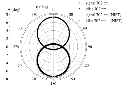
Figure 2: Polar plot of phase matching curves in a BBO crystal. Comparison of the approximated formula (24) with the “exact” phase matching formula, calculated with the method in NIST (NIST). $\theta$ is the polar angle from the pump direction of propagation, $\phi$ is the azymuthal angle. $\lambda_{signal}=\lambda_{idler}=702nm$. ($\lambda_{pump}=351nm$), and the pump propagates at an angle of $49.6$ degrees from the crystal optical axis

The equation $\Delta(\vec{q},\Omega)=0$ defines in the $(q_{x},q_{y})$ plane a circonference, centered at the position

$$q_{x}=0,\quad q_{y}=q_{C}=\frac{1}{2}q_{0}^{2}\rho_{e}l_{c}$$ (29)

and with radius given by

$$q_{R}=q_{0}\sqrt{\Delta_{0}+\frac{q_{C}^{2}}{q_{0}^{2}}+\Omega\tau_{coh}+\frac{1}{2}\epsilon(\Omega\tau_{coh})^{2}}\>.$$ (30)

This corresponds to the phase matched modes for the signal (ordinary) wave. Phase matched modes for the idler wave, emitted at the frequency $-\Omega$, lye on the symmetric circonference.
Figure 2 plots some examples of this phase matching circles, in the form of polar plot, with $\theta$ being the polar angle from the pump direction ($z$ axis) outside the crystal and $\phi$ the azymutal angle around $z$. Parameters are those of a BBO crystal, cut for degenerate phase matching at $49.6$ degrees, for a pump wavelength of $351$ nm. They have been calculated with the help of empirical Sellmeier formulas for refraction indices in Ref.Sellmeier . For comparison, superimposed to the curves calculated by means of Eq.(24), the figure shows the “exact” phase matching curves, calculated with the method described in NIST , by means of a public domain numerical routine available at NISTweb . The plots show a rather good agreement, in any case within the error inplicit in the use of empirical Sellmeier formulas.

III Polarization correlation: quantum field formalism

III.1 Stokes operators:definition and properties

Quantum-optical polarization properties of light are conveniently described within the formalism of Stokes operators, which represent the quantum conterparts of the Stokes vectors of classical optics. The polarization state of a classical beam can be described by means of a Stokes vector, and of its associated Poincarè sphere. Stokes vectors pointing on the equator of the sphere represents linearly polarized light; if the vector points in the positive (negative) directon of $S_{1}$ the light is horizontally (vertically) polarized, while the $S_{2}$ direction identifies light polarized at 45 (-45) degrees. The $S_{3}$ direction corresponds to circulary (right and left) polarized light. A fourth parameter, $S_{0}$ is the total beam intensity, and gives the radius of the Poincarè sphere. For a polarized beam $S_{1}^{2}+S_{2}^{2}+S_{3}^{2}=S_{0}^{2}$, so that the polarization state is represented by a point on the sphere surface.
In the quantum mechanical description of light polarization, Stokes parameters are replaced by a set of four Stokes operators. For a single mode of an electromagnetic field, they are defined in terms of the photon annihilation operators for a vertical and horizontal linear polarization mode $\hat{a}_{H},\hat{a}_{V}$, as:

$$\hat{S}_{0} = \hat{a}^{\dagger}_{H}\hat{a}_{H}+\hat{a}^{\dagger}_{V}\hat{a}_{V}$$ (31)

$$\hat{S}_{1} = \hat{a}^{\dagger}_{H}\hat{a}_{H}-\hat{a}^{\dagger}_{V}\hat{a}_{V}$$ (32)

$$\hat{S}_{2} = \hat{a}^{\dagger}_{H}\hat{a}_{V}+\hat{a}^{\dagger}_{V}\hat{a}_{H}=\hat{a}^{\dagger}_{45}\hat{a}_{45}-\hat{a}^{\dagger}_{-45}\hat{a}_{-45}$$ (33)

$$\hat{S}_{3} = -{\rm i}\left(\hat{a}^{\dagger}_{H}\hat{a}_{V}-\hat{a}^{\dagger}_{V}\hat{a}_{H}\right)=\hat{a}^{\dagger}_{R}\hat{a}_{R}-\hat{a}^{\dagger}_{L}\hat{a}_{L}\>,$$ (34)

where $\hat{a}_{45}$ , $\hat{a}_{-45}$ denote annihilation operators on the oblique polarization basis, and $a_{R}$ $a_{L}$ are annihilation operators on the circular right and circular left polarization basis. The first two operators represent, respectively, the sum and difference of photon numbers in the vertical/horizontal polarization basis. Operators $\hat{S}_{2}$ and $\hat{S}_{3}$ are the difference of photon numbers in the oblique and circular polarization basis, respectively. All these observables can be measured by means of a polarizing beam splitter and quarter and half wave plates, as e.g. described in BornWolf . However, while operator $\hat{S}_{0}$ commutes with all the others, the remaining three do not:

$$[\hat{S}_{1},\hat{S}_{2}]=2{\rm i}\hat{S}_{3}\>,\quad[\hat{S}_{2},\hat{S}_{3}]=2{\rm i}\hat{S}_{1}\>,\quad[\hat{S}_{3},\hat{S}_{1}]=2{\rm i}\hat{S}_{2}\;.$$ (35)

The set of Stokes operators has angular momentum-like commutation relation, and the associated observables are in general non compatible. The quantum state of a light beam cannot be any more visualized as a point on the Poincaré sphere, since quantum noise introduces a minimum uncertainty in the values of the Stokes parameter. Polarization squeezed states, whose uncertainty can be represented by an ellipsoid (see e.g. Korolkova ) has been recently realized Bowen .

III.2 Stokes operator correlation in the far field of parametric down-conversion

The main idea of this paper is to study the quantum correlation between Stokes operators measured from symmetric portions of the far field beam cross-section. To this end, we consider a measurement of the Stokes operators over a small region $D(\vec{x})$ centered around a position $\vec{x}$ in the far-field plane of the down-converted field, and over a detection time $T$ (tpically we will take $T$ much larger than the crystal coherence time).

$$\hat{S}_{i}(\vec{x})=\int_{T}dt^{\prime}\int_{D(\vec{x})}d\vec{x}^{\,\prime}\hat{\sigma}_{i}(\vec{x}^{\,\prime},t^{\prime})\;,$$ (36)

where

$$\hat{\sigma}_{0}(\vec{x},t) = \hat{A}_{o}^{\dagger}(\vec{x},t)\hat{A}_{e}(\vec{x},t)+\hat{A}_{o}^{\dagger}(\vec{x},t)\hat{A}_{e}(\vec{x},t)\;,$$ (37)

$$\hat{\sigma}_{1}(\vec{x},t) = \hat{A}_{o}^{\dagger}(\vec{x},t)\hat{A}_{o}(\vec{x},t)-\hat{A}_{e}^{\dagger}(\vec{x},t)\hat{A}_{e}(\vec{x},t)\>,$$ (38)

$$\hat{\sigma}_{2}(\vec{x},t) = \hat{A}_{o}^{\dagger}(\vec{x},t)\hat{A}_{e}(\vec{x},t)+\hat{A}_{e}^{\dagger}(\vec{x},t)\hat{A}_{o}(\vec{x},t)\;,$$ (39)

$$\hat{\sigma}_{3}(\vec{x},t) = -{\rm i}\left[\hat{A}_{o}^{\dagger}(\vec{x},t)\hat{A}_{e}(\vec{x},t)-\hat{A}_{o}^{\dagger}(\vec{x},t)\hat{A}_{e}(\vec{x},t)\right]\>.$$ (40)

$\hat{A}_{o/e}$ denotes the field operator for the ordinary/extraordinary polarized beam in the far-field plane, which can be observed in the focal plane of a lens, placed as shown in figure 3.
By using the free field commutation relations (12), it can be easily shown that

$$[\hat{S}_{1}(\vec{x}),\hat{S}_{2}(\vec{x})]=2{\rm i}\hat{S}_{3}(\vec{x})\>,\quad[\hat{S}_{2}(\vec{x}),\hat{S}_{3}(\vec{x})]=2{\rm i}\hat{S}_{1}(\vec{x})\>,\quad[\hat{S}_{3}(\vec{x}),\hat{S}_{1}(\vec{x})]=2{\rm i}\hat{S}_{2}(\vec{x})\;,$$ (41)

while operators measured from different (and not connected) detection pixels commute.

In the following, we shall consider Stokes operator correlation functions of the form:

$$\langle\delta\hat{S}_{i}(\vec{x})\,\delta\hat{S}_{j}(\vec{x}^{\,\prime})\rangle=\langle\hat{S}_{i}(\vec{x})\,\hat{S}_{j}(\vec{x}^{\,\prime})\rangle-\langle\hat{S}_{i}(\vec{x})\rangle\,\langle\,\hat{S}_{j}(\vec{x}^{\,\prime})\rangle\>,\qquad(i,j=0,\ldots 3)\>.$$ (42)

A useful tool for calculation are the correlation functions of the Stokes operator densities (37-40) :

$$G_{ij}(\vec{x},\vec{x}^{\,\prime};\tau)=\langle\hat{\sigma}_{i}(\vec{x},t+\tau)\,\hat{\sigma}_{j}(\vec{x}^{\,\prime},t)\rangle-\langle\hat{\sigma}_{i}(\vec{x},t+\tau)\rangle\,\langle\,\hat{\sigma}_{j}(\vec{x}^{\,\prime},t)\rangle$$ (43)

and their spectral densities

$$\tilde{G}_{ij}(\vec{x},\vec{x}^{\,\prime};\Omega)=\int d\tau{\rm e}^{{\rm i}\Omega\tau}G_{ij}(\vec{x},\vec{x}^{\,\prime};\tau)$$ (44)

Their relation with the correlation functions of the measured Stokes operator (42) is given by:

$$\langle\delta\hat{S}_{i}(\vec{x})\,\delta\hat{S}_{j}(\vec{x}^{\,\prime})\rangle=\int_{D(\vec{x})}d{\vec{x}}_{1}\int_{D(\vec{x}^{\,\prime})}d{\vec{x}}_{1}^{\,\prime}\int d\Omega\frac{T^{2}}{2\pi}{\rm sinc}^{2}\left(\Omega\frac{T}{2}\right)\tilde{G}_{ij}\left(\vec{x}_{1},\vec{x}_{1}^{\,\prime};\Omega\right)\>.$$ (45)

We notice that:

$$\lim_{T\to\infty}\frac{T}{2\pi}{\rm sinc}^{2}\left(\Omega\frac{T}{2}\right)=\delta(\Omega)\;,$$ (46)

and that this function acts under the integral as a frequency filter with bandwidth $\Delta\Omega=2\pi/T$. We shall assume in the following that the detection time is much larger than the crystal coherence time. Under this assumption

$$\langle\delta\hat{S}_{i}(\vec{x})\,\delta\hat{S}_{j}(\vec{x}^{\,\prime})\rangle\stackrel{{\scriptstyle T\gg\tau_{coh}}}{{\longrightarrow}}T\int_{D(\vec{x})}d{\vec{x}}_{1}\int_{D(\vec{x}^{\,\prime})}d{\vec{x}}_{1}^{\,\prime}\tilde{G}_{ij}\left(\vec{x}_{1},\vec{x}_{1}^{\,\prime};\Omega=0\right)$$ (47)

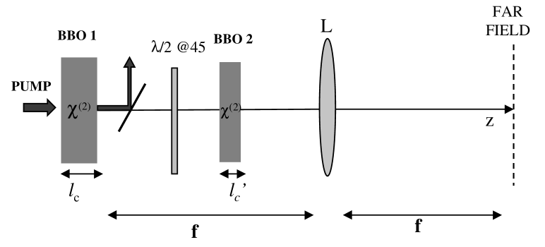
Figure 3: Schematic set-up for a measurement in the far field plane with a compensation crystal. BBO1, down-conversion crystal of length $l_{c}$; $\lambda/2@45$ half-wave plate, rotates polarization by 90 degrees; BBO2, compensation crystal of length $l_{c}^{\prime}$, $L$ lens of focal length $f$.

When a lens of focal length $f$ is placed at a focal distance both from the crystal output plane and the observation plane (see figure 3), the field operators in the far-field plane are connected to those at the crystal output by the usual mapping Goodman

$$\hat{A}_{i}(\vec{x},\Omega)=\frac{2\pi}{{\rm i}\lambda_{i}f}\hat{A}_{i}^{out}\left(\vec{q}=\frac{2\pi\vec{x}}{\lambda_{i}f},\Omega\right)\;,$$ (48)

where $f$ is the focal length of the lens used to image the far field plane and $\lambda_{i}$ is the wavelength (in vacuum) at the frequency $\omega_{p}/2+\Omega$.
Since the light statistics is Gaussian (the output operators are obtained by a linear transformation acting on input vacuum field operators) all expectation values and correlation functions of interest can be calculated by making use of the second order moments of field operators. These can be easily calculated in the far field plane by assuming that the down-converted field operators at the input crystal face are in the vacuum state and by using the input/output relations (11), toghether with (48), thus obtaining

$$\left\langle\hat{A}_{i}^{\dagger}(\vec{x},\Omega)\hat{A}_{j}(\vec{x}^{\,\prime},\Omega^{\,\prime})\right\rangle = \delta_{i,j}\delta(\vec{x}-\vec{x}^{\,\prime})\,\delta(\Omega-\Omega^{\,\prime})\left|{\cal V}_{i}(\vec{x},\Omega)\right|^{2}\>,$$ (49)

$$\left\langle\hat{A}_{i}(\vec{x},\Omega)\hat{A}_{j}(\vec{x}^{\,\prime},\Omega^{\,\prime})\right\rangle = -\frac{\lambda_{j}}{\lambda_{i}}(1-\delta_{i,j})\delta(\vec{x}\frac{\lambda_{j}}{\lambda_{i}}+\vec{x}^{\,\prime})\,\delta(\Omega+\Omega^{\,\prime}){\cal U}_{i}(\vec{x},\Omega){\cal V}_{j}(-\vec{x}\frac{\lambda_{j}}{\lambda_{i}},-\Omega)\>,\qquad(i,j=o,e)\;.$$ (50)

In this formula

$${\cal U}_{i}(\vec{x},\Omega)=U_{i}\left(\vec{q}=\vec{x}\frac{2\pi}{\lambda_{i}f},\Omega\right)\>,\qquad{\cal V}_{i}(\vec{x},\Omega)=V_{i}\left(\vec{q}=\vec{x}\frac{2\pi}{\lambda_{i}f},\Omega\right)$$ (51)

where $U_{i},V_{i}$ are are the gain functions defined by (17–22). It can be noticed the presence of the nonzero “anomalous” propagator (50), a term which is characteristic of processes where particles are created in pairs. In order to simplify the notation, in the following we shall consider the case $\Omega<<\omega_{p}/2$, and take $\lambda_{o}=\lambda_{e}=\lambda=2\lambda_{p}$. In a real experimental implementation, however, the validity of such an approximation should be carefully checked when not using narrow frequency filters; twin photons produced at different wavelengths $\lambda_{e}$, $\lambda_{o}$, and travelling with symmetric $\vec{q}$, $-\vec{q}$ transverse wave vectors are actually propagating at different angles from the pump and will be intercepted in the far field at two sligtly different radial positions.
The fact that the field spatial correlation are perfectly localized in the far field (the Dirac-delta form of the correlation peak) is a consequence of the traslational symmetry of the model in the transverse plane (plane wave pump and a crystal slab infinite in the transverse direction). A trivial formal fault is that the far field mean intensity of the downconverted beams diverges, as a consequence of the infinite energy of a plane-wave pump. This artificial divergence can be formally eliminated with the trick used in Kolobov99 ; Brambilla , where a finite size pupil was inserted at the output face of the crystal. The spatial Dirac-delta functions in Eqs.(49,50) are substituted by a finite version, and a typical resolution area, proportional to the diffraction spot of the pupil in the far field plane, is introduced in the scheme. For a pupil of transverse area $S_{P}$, this is given by $D_{R}=(\lambda f)^{2}/S_{P}$. The typical scale of variation of the gain functions (51) in the far field plane is

$$X_{0}=q_{0}\lambda f/(2\pi)\>;$$ (52)

when $X_{0}$ is much larger than the resolution area (or, equivalently, when the pupil size is much larger than the amplifier coherence length), the mean photon number distribution in the far field plane is given by

$$\langle\hat{N}_{i}(\vec{x})\rangle = \int_{D(\vec{x})}d\vec{x}^{\,\prime}\int_{T}dt\langle\hat{A}^{\dagger}_{i}(\vec{x}^{\,\prime},t)\hat{A}_{i}(\vec{x}^{\,\prime},t)\rangle=$$ (53)

$$\approx \frac{T}{D_{R}}\int_{D(\vec{x})}d\vec{x}^{\,\prime}\int\frac{d\Omega}{2\pi}\left|{\cal V}_{i}(\vec{x}^{\,\prime},\Omega)\right|^{2}\>,$$

When the finite size of the pump is taken into account in a numerical model Brambilla02 , it is easily seen that the resolution area is rather given in terms of the spot size of the pump as it is imaged in the far field plane. For a Gaussian pump of waist $w_{p}$, $D_{R}\approx(\lambda f)^{2}/(\pi w_{p}^{2})$.

In this limit of small resolution area, the mean value of Stokes operators is given by:

$$\langle\hat{S}_{0}(\vec{x})\rangle = \frac{T}{D_{R}}\int_{D(\vec{x})}d\vec{x}^{\,\prime}\int\frac{d\Omega}{2\pi}\left[\left|{\cal V}_{o}(\vec{x}^{\,\prime},\Omega)\right|^{2}+\left|{\cal V}_{e}(\vec{x}^{\,\prime},\Omega)\right|^{2}\right]$$ (54)

$$\langle\hat{S}_{1}(\vec{x})\rangle = \frac{T}{D_{R}}\int_{D(\vec{x})}d\vec{x}^{\,\prime}\int\frac{d\Omega}{2\pi}\left[\left|{\cal V}_{o}(\vec{x}^{\,\prime},\Omega)\right|^{2}-\left|{\cal V}_{e}(\vec{x}^{\,\prime},\Omega)\right|^{2}\right]$$ (55)

$$\langle\hat{S}_{2}(\vec{x})\rangle = \langle\hat{S}_{3}(\vec{x})\rangle=0$$ (56)

III.3 Correlation in Stokes operators $S_{1},S_{0}$

The first and second Stokes operators represent the sum and the difference, respectively, between the number of ordinary and extraordinary photons (say horizontally and vertically polarized photons) measured from a detection pixel in the far field plane.

$$\hat{S}_{0}(\vec{x}) = \hat{N}_{o}(\vec{x})+\hat{N}_{e}(\vec{x})\;$$ (57)

$$\hat{S}_{1}(\vec{x}) = \hat{N}_{o}(\vec{x})-\hat{N}_{e}(\vec{x})$$ (58)

The plane wave pump model predicts that the number of ordinary and extraordinary photons collected from any two symmetric portions of the far field plane are perfectly correlated observables Brambilla02 ; Brambilla . This result is a direct consequence of pairwise emission of photons with horizontal (ordinary) and vertical (extraordinary) polarizations, propagating in symmetric directions, as required by transverse light momentum conservation. Hence, this model predicts an ideally perfect correlation, both between $\hat{S}_{0}(\vec{x})$, $\hat{S}_{0}(-\vec{x})$, and between $\hat{S}_{1}(\vec{x})$, $-\hat{S}_{1}(-\vec{x})$ for any choice of the position $\vec{x}$ in the far field (notice that $\hat{S}_{0}(\vec{x})$ commutes with $\hat{S}_{1}(\vec{x}^{\prime})$).
In a more sofisticated numerical model Brambilla02 , it is readily seen that the finite width of the pump profile introduces an uncertainty in the directions of propagation of the down-converted photons. As described by the propagation equation (4), when a $o$ photon is emitted in direction $\vec{q}$, its twin $e$ photon is emitted in the direction $-\vec{q}$ within an uncertainty $\delta q\propto 2/w_{p}$, which is the bandwidth of the pump spatial Fourier transform. A photon number correlation well beyond the shot noise level is recovered when photons are collected from regions larger than a resolution area $D_{R}\approx\pi\left(\delta q\frac{\lambda f}{2\pi}\right)^{2}=(\lambda f)^{2}/(\pi w_{p}^{2})$.

In the limit of a small resolution area, long but straigthforward calculations calc show that:

$$\tilde{G}_{00}(\vec{x},\vec{x}^{\,\prime};\Omega) = \frac{1}{D_{R}}\left[\delta(\vec{x}-\vec{x}^{\,\prime})F_{1}(\vec{x},\Omega)+\delta(\vec{x}+\vec{x}^{\,\prime})F_{2}(\vec{x},\Omega)\right]$$ (59)

$$\tilde{G}_{11}(\vec{x},\vec{x}^{\,\prime};\Omega) = \frac{1}{D_{R}}\left[\delta(\vec{x}-\vec{x}^{\,\prime})F_{1}(\vec{x},\Omega)-\delta(\vec{x}+\vec{x}^{\,\prime})F_{2}(\vec{x},\Omega)\right]$$ (60)

with

$$F_{1}(\vec{x},\Omega) = \int\frac{d\omega}{2\pi}\left\{\left|{\cal V}_{o}(\vec{x},\omega){\cal U}_{o}(\vec{x},\omega+\Omega)\right|^{2}+\left|{\cal V}_{e}(\vec{x},\omega){\cal U}_{e}(\vec{x},\omega+\Omega)\right|^{2}\right\}$$ (61)

$$F_{2}(\vec{x},\Omega) = \int\frac{d\omega}{2\pi}\left\{{\cal U}_{o}(\vec{x},\omega){\cal U}_{o}^{*}(\vec{x},\omega-\Omega){\cal V}_{e}(-\vec{x},-\omega){\cal V}_{e}^{*}(-\vec{x},-\omega+\Omega)\right.$$ (62)

$$+ \left.{\cal U}_{e}(\vec{x},\omega){\cal U}_{e}^{*}(\vec{x},\omega-\Omega){\cal V}_{o}(-\vec{x},-\omega){\cal V}_{0}^{*}(-\vec{x},-\omega+\Omega)\right\}$$

The correlation functions have two peaks; the first one, located at $\vec{x}^{\,\prime}=\vec{x}$, accounts for the noise in the measurement of Stokes parameter from a single pixel. The second one is located at $\vec{x}^{\,\prime}=-\vec{x}$ and accounts for correlation (anticorrelation) between measurements performed over symmetric pixels. By taking into account the unitarity relations (13,15), it can be immediately noticed that when $\Omega=0$ (corresponding to long detection times) $F_{1}(\vec{x},0)=F_{2}(\vec{x},0)$, and the two corelation function peaks have the same size. This represents the maximum amount of correlation allowed by Schwarz inequality, which requires that

$$\left|\langle\delta\hat{S}_{i}(\vec{x})\,\delta\hat{S}_{i}(-\vec{x})\rangle\right|\leq\left[\langle\delta\hat{S}_{i}(\vec{x})\,\delta\hat{S}_{i}(\vec{x})\rangle\langle\delta\hat{S}_{i}(-\vec{x})\,\delta\hat{S}_{i}(-\vec{x})\rangle\right]^{\frac{1}{2}}$$ (63)

In our case, assuming two symmetric detection pixels $D(\vec{x})$ and $D(-\vec{x})$, we have e.g.

$$\langle\delta\hat{S}_{1}(\vec{x})\,\delta\hat{S}_{1}(\vec{x})\rangle = \langle\delta\hat{S}_{1}(-\vec{x})\,\delta\hat{S}_{1}(-\vec{x})\rangle=\frac{T}{D_{R}}\int_{D(\vec{x})}d\vec{x}^{\,\prime}F_{1}(\vec{x}^{\,\prime},0)$$ (64)

$$\langle\delta\hat{S}_{1}(\vec{x})\,\delta\hat{S}_{1}(-\vec{x})\rangle = -\frac{T}{D_{R}}\int_{D(\vec{x})}d\vec{x}^{\,\prime}F_{2}(\vec{x}^{\,\prime},0)=-\langle\delta\hat{S}_{1}(\vec{x})\,\delta\hat{S}_{1}(\vec{x})\rangle$$ (65)

Finally, the existence of such a perfect correlation implies that both $\hat{S}_{1}(\vec{x})+\hat{S}_{1}(-\vec{x})$ and $\hat{S}_{0}(\vec{x})-\hat{S}_{0}(-\vec{x})$ are noiseless observables. For example:

$$\langle\left[\delta\hat{S}_{1}(\vec{x})+\delta\hat{S}_{1}(-x)\right]^{2}\rangle = 2\left[\langle\delta\hat{S}_{1}(\vec{x})\,\delta\hat{S}_{1}(\vec{x})\rangle+\langle\delta\hat{S}_{1}(\vec{x})\,\delta\hat{S}_{1}(-\vec{x})\rangle\right]=0$$ (66)

III.4 Correlation in Stokes operators $S_{2},S_{3}$

Quite different is the situation for the other two Stokes operators $S_{2},S_{3}$, which involve measurements of the photon number in a polarization basis different from the ordinary and extraordinary ones of the crystal, namely in the oblique and circular polarization basis.
Calculations along the same lines of those performed for the first two Stokes operators show that also in this case the correlation functions display two peaks, one representing the noise associated to the measurement over a single pixel, the other the correlation between symmetric pixels.

$$\tilde{G}_{22}(\vec{x},\vec{x}^{\,\prime};\Omega) = \tilde{G}_{33}(\vec{x},\vec{x}^{\,\prime};\Omega)$$ (67)

$$= \frac{1}{D_{R}}\left[\delta(\vec{x}-\vec{x}^{\,\prime})H_{1}(\vec{x},\Omega)+\delta(\vec{x}+\vec{x}^{\,\prime})H_{2}(\vec{x},\Omega)\right]$$ (68)

with

$$H_{1}(\vec{x},\Omega) = \int\frac{d\omega}{2\pi}\left\{\left|{\cal V}_{o}(\vec{x},\omega){\cal U}_{e}(\vec{x},\omega+\Omega)\right|^{2}+\left|{\cal V}_{e}(\vec{x},\omega){\cal U}_{o}(\vec{x},\omega+\Omega)\right|^{2}\right\}$$ (69)

$$H_{2}(\vec{x},\Omega) = \int\frac{d\omega}{2\pi}\left\{{\cal U}_{o}^{*}(\vec{x},\omega){\cal U}_{e}(\vec{x},\omega+\Omega){\cal V}_{e}^{*}(-\vec{x},-\omega){\cal V}_{o}(-\vec{x},-\omega-\Omega)\right.$$ (70)

$$+ \left.{\cal U}_{e}^{*}(\vec{x},\omega){\cal U}_{o}(\vec{x},\omega+\Omega){\cal V}_{o}^{*}(-\vec{x},-\omega){\cal V}_{e}(-\vec{x},-\omega-\Omega)\right\}$$

However, at difference with the previous case, the two peaks in general do not have the same size, even for a long measurement time. Letting $\Omega=0$ in Eqs. (69, 70) and using the definition (17), which is a consequence of unitarity, we have

$$H_{1}(\vec{x},0) = \int\frac{d\omega}{2\pi}\left\{\left|{\cal V}(\vec{x},\omega){\cal U}(-\vec{x},-\omega)\right|^{2}+\left|{\cal V}(-\vec{x},-\omega){\cal U}(\vec{x},\omega)\right|^{2}\right\}$$ (71)

$$H_{2}(\vec{x},0) = \int\frac{d\omega}{2\pi}2{\rm Re}\left\{{\cal U}^{*}(\vec{x},\omega){\cal U}(-\vec{x},-\omega){\cal V}^{*}(\vec{x},\omega){\cal V}(-\vec{x},-\omega)\right\}\;,$$ (72)

$$H_{1}(\vec{x},0)-H_{2}(\vec{x},0) = \int\frac{d\omega}{2\pi}\left|{\cal V}^{*}(\vec{x},\omega){\cal U}(-\vec{x},-\omega)-{\cal V}^{*}(-\vec{x},-\omega){\cal U}(\vec{x},\omega)\right|^{2}$$ (73)

where ${\cal U},{\cal V}$ appearing in these equations are the functions defined by Eqs.(19,20), calculated at $\vec{q}=\vec{x}2\pi/(\lambda f)$. Moreover,

$$\langle\left[\hat{S}_{2}(\vec{x})-\hat{S}_{2}(-\vec{x})\right]^{2}\rangle = \langle\left[\hat{S}_{3}(\vec{x})-\hat{S}_{3}(-\vec{x})\right]^{2}\rangle$$ (74)

$$= \frac{2T}{D_{R}}\int_{D(\vec{x})}d\vec{x}^{\,\prime}\left[H_{1}(\vec{x}^{\,\prime},0)-H_{2}(\vec{x}^{\,\prime},0)\right]$$ (75)

The noise in the difference between Stokes operators measured from symmetric pixels in general does not vanish, due to the lack of symmetry $\vec{x},\Omega\to-\vec{x},-\Omega$ in the gain functions. In turns, this reflects the effect of spatial walk-off between the ordinary/extraordinary beams (described by the term proportional to $q_{y}$ in the phase mismatch function 24) and the group velocity mismatch beteween the two waves (described by the term proportional to $\Omega$ in 24).

III.4.1 Narrow-band frequency filtering results

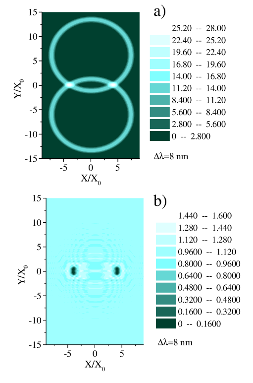
Figure 4: a) Far field photon number distribution of the down-converted field. b)Distribution of the noise in the difference between $\hat{S}_{2}$ measured from symmetric portions of the beam cross-section, scaled to the shot-noise level. The distribution for $\hat{S}_{3}$ is identical. A step function frequency filter $\Delta\lambda=8$ nm wide, centered around the degenerate frequency is used in both plots. $\sigma=2$

Part (b) of Fig.4 shows a typical result for the noise in the difference between Stokes operators measured from small (but larger than $D_{R}$) symmetric portions of the far-field. Precisely, the figure shows $\langle\left[\hat{S}_{2}(\vec{x})-S_{2}(-\vec{x})\right]^{2}\rangle=\langle\left[\hat{S}_{3}(\vec{x})-S_{3}(-\vec{x})\right]^{2}\rangle$, scaled to the shot noise level, represented by $\langle\left[\hat{S}_{0}(\vec{x})+S_{0}(-\vec{x})\right]\rangle$, as a function of the transverse coordinate $\vec{x}=(x,y)$ scaled to $X_{0}$. Parameters in this plot are those of a 2 mm long BBO crystal, cut at $49.6$ degrees for degenerate type II phase matching at $702\rm{nm}$. For comparison, part (a) of the figure shows the mean photon number distribution in the far field. The numbers associated with the scale in (a) represent the number of photons detected over a resolution area $D_{R}$ and over a crystal coherence time, that is the mean photon number per mode. Both plots have been obtained by filtering the emitted frequencies in a bandwidth $\Delta\lambda=8$ nm wide around the degenerate frequency, by means of a step function filter. Precisely, we let

$$\hat{A}_{i}(\vec{x},\Omega)\to\sqrt{f(\Omega)}\hat{A}_{i}(\vec{x},\Omega)+\sqrt{1-f(\Omega)}\hat{v}_{i}(\vec{x},\Omega)\quad i=o,e\;,$$ (76)

where $\hat{v}_{i}(\vec{x},\Omega)$ are vacuum field operators uncorrelated from the signal and idler fields $\hat{A}_{i}(\vec{x},\Omega)$, and the filter function $f(\Omega)$ is this case the step function $f(\Omega)=1$ for $\Omega\epsilon[-\frac{\Delta\Omega}{2},\frac{\Delta\Omega}{2}]$, $f(\Omega)=0$ elsewhere.

In plot (b) we see clearly two large dark zones, in correspondence of the intersections of the emission cones, where the Stokes operator correlation is almost perfect. Out of these regions, basically no spatial correlation at the quantum level exists for Stokes operator $S_{2}$ and $S_{3}$.
Remarkably, at the intersection of the two degenerate emission cones, the light is completly unpolarized. Figure 5 shows the distribution of $\langle\hat{S}_{1}(\vec{x})\rangle/\langle\hat{S}_{0}(\vec{x})\rangle$ in the transverse far-field plane, showing that it vanishes at the emission ring intersection; recalling that the mean value of $\hat{S}_{2}$ and $\hat{S}_{3}$ is zero everywhere, this means a vanishing degree of polarization in these regions. Moreover, in these regions a measurement of Stokes parameters over a single detection pixel is very noisy, as shown by figure 6, which plots the distribution of $\langle[\delta\hat{S}_{2}(\vec{x})]^{2}\rangle=\langle[\delta\hat{S}_{3}(\vec{x})]^{2}\rangle$, scaled to the shot noise level $\langle\hat{S}_{0}(\vec{x})\rangle$. In this plot the uniform dark background correponds to the shot noise level, while the bright spots correspond to a noise level 10-12 times larger than the shot noise.

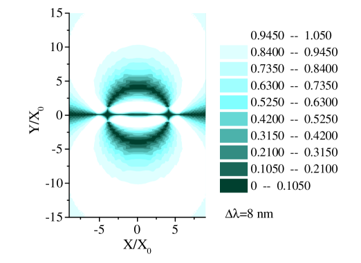
Figure 5: Degree of polarization of the light downconverted by a BBO crystal. Far field distribution of $\langle\hat{S}_{1}(\vec{x})\rangle/\langle\hat{S}_{0}(\vec{x})\rangle$. Same parameters as in Fig.4

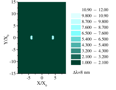
Figure 6: Noise in the measurement of Stokes parameters of the downconverted light by a BBO crystal. Far field distribution of $\langle[\delta\hat{S}_{2}(\vec{x})]^{2}\rangle/\langle\hat{S}_{0}(\vec{x})\rangle=\langle\hat{[}\delta S_{3}(\vec{x})]^{2}\rangle/\langle\hat{S}_{0}(\vec{x})\rangle$. Same parameters as in Fig.4

Similar results are obtained in any gain regime. In the small gain limit, the noise statistics associated to a measurement over a single pixel becomes essentially Poissonian, but the correlation between Stokes parameters measured from symmetric pixels is basically the same as in the high gain regime. Fig. 7 compares the noise in the difference between Stokes parameters measured from symmetric pixels in the small and high gain regimes, plotted as a function of the vertical coordinate along the circle of maximum gain for the degenerate frequency. The dashed lines were obtained with $\sigma=0.01$, corresponding to a mean photon number per mode $\approx 10^{-4}$, the solid lines with $\sigma=2$, corresponding to a mean photon number per mode $\approx 15$ (see Fig.4a),. In this plot, the two dark lines are, as usual, obtained by filtering the frequencies with a step function ($\Delta\lambda=5$nm). For comparison, the two light lines show the results obtained by means of a more realistic frequency filter, with a Gaussian profile. Precisely, we take the filter function in Eq.(76) as $f(\Omega)=\exp{\left[-(\Omega^{2}4{\rm ln}2)/(\Delta\Omega^{2})\right]}$ where $\Delta\Omega$ is the full width at half maximum (FWHM), and corresponds to an interval in wavelengths of 5nm. In this case, losses introduced by the Gaussian shape of the filter slightly deteriorates the correlation.

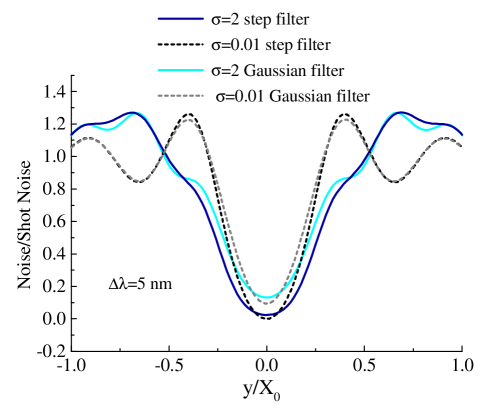
Figure 7: Noise in the difference between $\hat{S}_{2}$ ($\hat{S}_{3}$) measured from symmetric portions of the beam cross-section, scaled to the shot-noise level, as a function of the vertical coordinate $y$ along the maximum gain circle for the degenerate frequency. Dashed lines: $\sigma=0.01$, solid lines $\sigma=2$ Light lines: Gaussian frequency filter, of FWHM = 5nm. Dark lines: step function filter 5nm wide.

The results described above were obtained by exploiting a trick commonly used in the experiments performed in the single photon pair regime ( for example in the experiment of kwiat ), in order to partially compensate for the temporal and spatial walk-off of the down-converted beams. In the regime of single photon pair production, the ordinary and extraordinary photons can be in principle distinguished because of their different group velocities inside the crystal, and because of their offsets in propagation directions due to walk-off effects inside the crystal. The mere existence of this possibility is detrimental for the entanglement of the state. As it is discussed in details in Appendix A, in the general case (arbitrary number of down-converted photons), the group velocity mismatch and the spatial walk-off are responsible for the appearance of a propagation phase factor that lower the value of the correlation function between Stokes operators measured from symmetric regions. In principle, this problem can be solved by using a vey narrow frequency filter, and by performing the measurement over narrow regions centered around the ring intersections. However, this lower the efficiency of the set up. An other possibility is to insert a second crystal, after the pump beam has been removed, and after the field polarization has been rotated by $90^{0}$ (see Fig.3). In this way, the slow and fast wave in the first crystal become the fast and slow wave, respectively, in the second crystal, and the direction of walk-off is reversed. At difference from the single photon pair regime, the correlation is optimized when the length of this second crystal is chosen as

$$l^{\prime}_{c}=l_{c}\frac{\tanh\sigma}{2\sigma}\>,$$ (77)

where $\sigma$ is the linear gain parameter, proportional to the pump amplitude and to the first crystal length (see Appendix A). The fact that the optimal length of the compensation crystal decreases with increasing gain can be understood as following John ; Bahaa : in the regime of single photon pair production (limit $\sigma\to 0$), the photon pair can be produced at any point along the crystal length with uniform probability, so that the average temporal delay of the two photons due to the group velocity mismatch are those corresponding to half of the crystal length, and best compensation is achieved for $l^{\prime}_{c}=\frac{l_{c}}{2}$. In the large gain regime, more and more photon pairs are produced towards the end of the crystal (the number of down-converted photons increases exponentially with the crystal length), so that walk-off effects are best compensated by a shorter crystal, whose length is given by formula (77).

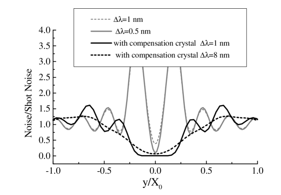
Figure 8: Effect of the compensation crystal. Noise in the difference between $\hat{S}_{2}$ measured from symmetric pixels, scaled to the shot-noise level. $y$ is the far-field vertical position along the maximum gain circle. Gray lines: without compensation crystal, dashed gray line $\Delta\lambda=1$nm, solid gray line $\Delta\lambda=0.5$nm. Black lines: with optimal compensation crystal, solid black line $\Delta\lambda=1$nm, dashed black line $\Delta\lambda=8$nm.

When this kind of optimization is not possible, our calculations show that similar results can be obtained by a narrow-band temporal and spatial filtering, and/or by using crystals that exhibit a smaller amount of walk-off. Figure 8 details the role of the compensation crystal. It plots the noise in the difference between Stokes parameters measured from symmetric pixels as a function of the vertical coordinate $y$ along the circle corresponding to the maximum gain at the degenerate frequency.

III.4.2 Broad-band frequency filtering results

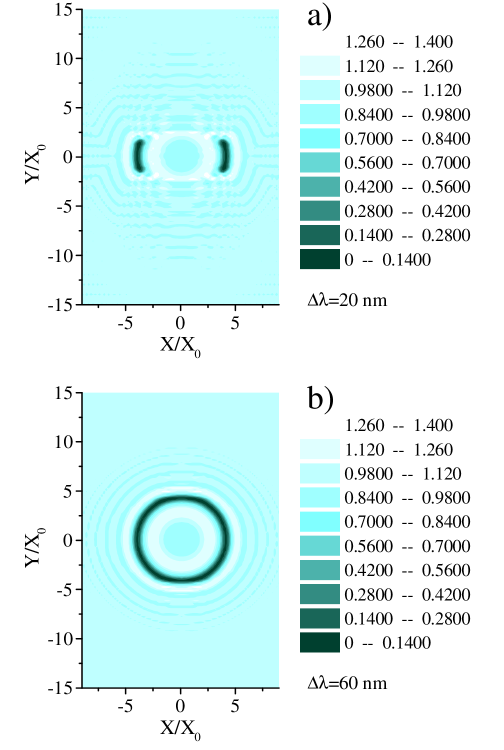
Figure 9: Broad-band frequency filtering. Distribution of the noise in the difference between $\hat{S}_{2}$ ($\hat{S}_{3}$) measured from symmetric portions of the beam cross-section, scaled to the shot-noise level. In part a) a frequency filter $\Delta\lambda=20$ nm wide, centered around the degenerate frequency is used; in b) $\Delta\lambda=60$ nm.

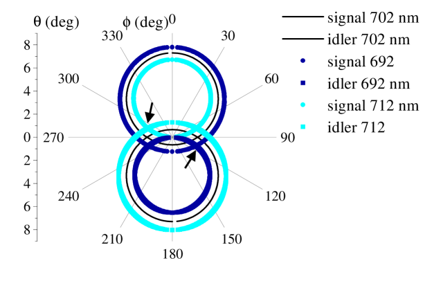
Figure 10: Polar plot of phase matching curves in a 2 mm BBO crystal cut at 49.6 degrees. $\theta$ is the polar angle from the pump direction of propagation; $\phi$ is the azymuthal angle around the pump. Black thin curves: $\lambda_{signal}=\lambda_{idler}=702nm$ Dark thick curves: $\lambda_{signal}=\lambda_{idler}=692nm$. Light thick curves:$\lambda_{signal}=\lambda_{idler}=712.29$ nm. The signal is the ordinary (slow) wave, and correspond to curves in the upper half of the plot. Idler is the extraordinary (fast) wave.

The results described in section III.4.1 were obtained by using relatively narrow frequency filters (5-8 nm). Remarkably, when a broader frequency filter is employed, the regions where Stokes parameter are correlated stretch to form a ring-shaped region around the pump direction (see Fig. 9). This kind of shape can be understood by considering the geometry of the downconversion cones emitted at the various frequencies by a BBO crystal. Figure 10 is a polar plot of the phase matching curves (geometrical loci of the phase matched modes), with $\theta$ being the polar angle from the pump direction of propagation ($z$ axis) and $\phi$ the azymuthal angle around $z$. In this plot the same color identifies the same emission wavelength; dark/light thick curves correspond to two conjugate wavelengths, while the thin black curves are the two emission cones at the degenerate wavelength. The signal (ordinary) wave emission curves are those in the upper half of the plot. When considering the intersection points of a dark circle with a light circle, which correspond to two conjugate wavelenghts, we cannot expect any kind of entanglement, since photons arriving in these positions are clearly distinguishable by their different frequencies. Let us consider, instead, one of the intersection of the light curves (e.g the one pointed by the arrow in the plot). Here ordinary and extraordinary photons arrive with identical probability, and have the same wavelength. As a consequence, the photon polarization is undetermined, and the light is completely unpolarized. However, each time an ordinary (extraordinary) photon arrives at this position, an extraordinary (ordinary) photon, at the conjugate wavelength, will be found at the symmetric position. This corresponds to the intersection of the two dark curves, indicated in the plot by the second arrow. Hence, when considering photodetection from the two regions indicated by the arrows in the plot we can expect a high degree of polarization entanglement. The same reasoning can be made for any of intesection of circles corresponding to the same wavelength (light with light, dark with dark and thin black with thin black). By connecting all these points toghether, we can for example recognize the geometrical shape of the dark regions in Fig.9a, where a high degree of correlation in all the Stokes parameters exists. By including more frequencies, the ring-shaped region if Fig. 9b shows up.
From the mathematical point of view, the form of the region where Stokes parameters are quantum correlated is given by the solution of the equation:

$$\Delta(\vec{q},\Omega)=\Delta(-\vec{q},-\Omega)=0$$ (78)

with $\vec{x}=2\pi\vec{q}/(\lambda f)$. By introducing the explicit form the the phase mismatch function 24, (78) is the equation of an ellipse (with a small eccentricity) centered around the origin, that is, the best correlated modes form a slightly asymmetric cone around the pump direction.

IV Polarization correlation: Quantum state formalism

This section is devoted to the discussion of the problem in terms of an equivalent quantum state formalism. Our aim is, on the one side, to give an alternative and istructive point of view on the problem, which can be compared with already existing quantum-state description of the problem (see e.g Bowmeester ). On the other side, we think that this section will show how the quantum field formalism developed in the first part of this paper is more powerful and strightforward, in terms of calculation efforts, than the commonly used quantum state formalism, at least for this kind of multi-mode problems.

Equation (11) defines a linear transformation acting on field operators, that maps field operators at the entrance face of the crystal into those at the output face. An equivalent transformation, acting on the quantum state of the signal/idler fields at the crystal input and mapping it into the state at the crystal output, is derived in details in Appendix B. As described in the appendix, in order to avoid formal difficulties coming from a continuum of modes, we have introduced a quantisation box both in the transverse spatial domain and in the temporal domain, so that the continuum of spatio-temporal modes $\vec{q},\Omega$ is replaced by a discrete set of modes.

When at the input of the parametric crystal there is the vacuum state for both signal and idler fields

$$\left|\psi\right\rangle_{in}=\left|vac\right\rangle=\prod_{\vec{q},\Omega}\left|0;-\vec{q},-\Omega\right\rangle_{o}\,\left|0;\vec{q},\Omega\right\rangle_{e}\;,$$ (79)

we find that the output state takes the form

$$\left|\psi\right\rangle_{out} = \prod_{\vec{q},\Omega}\left\{\sum_{n=0}^{\infty}c_{n}(\vec{q},\Omega)\left|n;\vec{q},\Omega\right\rangle_{o}\,\left|n;-\vec{q},-\Omega\right\rangle_{e}\right\}\;$$ (80)

$$c_{n}(\vec{q},\Omega) = \frac{1}{\cosh r(\vec{q},\Omega)}\left[\tanh r(\vec{q},\Omega)\right]^{n}{\rm e}^{2{\rm i}n\psi(\vec{q},\Omega)}=\frac{\left[U_{o}(\vec{q},\Omega)V_{e}(-\vec{q},-\Omega)\right]^{n}}{\left|U_{o}(\vec{q},\Omega)\right|^{2n+1}}\>,$$ (81)

where the notation $\left|n;\vec{q},\Omega\right\rangle_{o/e}$ indicates the Fock state with n photons in mode $(\vec{q},\Omega)$ of the ordinary/extraordinary polarized beam. Here the functions $U_{o},V_{e}$ are the coefficients of the operator transformation (11), and functions $r$ and $\psi$ are defined by Equations (17,18) toghether with (19, 20).
The state (81) is clearly entangled (non factorizable) with respect to the ordinary and extraordinary polarized beam components.

Let us focus on two conjugate modes $\vec{q},\Omega$ and $-\vec{q},-\Omega$ for both the ordinary and extraordinary field components. These can be for example observed by using a narrow filter around the degenerate frequency $\Omega=0$ and collecting light from two diaphragms placed around two symmetric regions in the far field zone. For brevity of notation, let us label these modes with the 3D vectors $\vec{\xi}=(q_{x},q_{y},\Omega)$, $-\vec{\xi}=(-q_{x},-q_{y},-\Omega)$. When restricted to these modes, the state takes the form

$$\left|\psi\right\rangle_{out}^{\vec{\xi}} = \left\{\sum_{n}c_{n}(\vec{\xi})\left|n;\vec{\xi}\right\rangle_{o}\,\left|n;-\vec{\xi}\right\rangle_{e}\right\}\left\{\sum_{n^{\,\prime}}c_{n^{\,\prime}}(-\vec{\xi})\left|n^{\,\prime};-\vec{\xi}\right\rangle_{o}\,\left|n^{\,\prime};\vec{\xi}\right\rangle_{e}\right\}$$ (82)

$$= \sum_{N=0}^{\infty}\left|\phi\right\rangle_{N}^{\vec{\xi}}$$ (83)

$$\left|\phi\right\rangle_{N}^{\vec{\xi}} = \sum_{m=0}^{N}\gamma_{N,m}(\vec{\xi})\left|m;\vec{\xi}\right\rangle_{o}\,\left|N-m;\vec{\xi}\right\rangle_{e}\left|N-m;-\vec{\xi}\right\rangle_{o}\,\left|m;-\vec{\xi}\right\rangle_{e}$$ (84)

where the last two lines have been obtained by changing the dummy summation variables $n,n^{\,\prime}$ into $m=n$, $N=n+n^{\,\prime}$.
The state can be represented as a superposition of states with a fixed total number of photons $N$. In each N-photon state described by Eq.(84)

$$\gamma_{N,m}(\vec{\xi}) = c_{m}(\vec{\xi})c_{N-m}(-\vec{\xi})$$ (85)

$$= \frac{[{\rm tanh}r(\vec{\xi})]^{m}[{\rm tanh}r(-\vec{\xi})]^{N-m}}{{\rm cosh}r(\vec{\xi})\,{\rm cosh}r(-\vec{\xi})}{\rm e}^{2{\rm i}N\psi(-\vec{\xi})}{\rm e}^{2{\rm i}m[\psi(\vec{\xi})-\psi(-\vec{\xi})]}$$

represents the probability amplitude of finding m ordinary photons, N-m extraordinary photons in mode $\vec{\xi}$, and N-m ordinary photons, m extraordinary photons in the conjugate mode $-\vec{\xi}$. The description of the state given by Eqs.(82-84) is a generalization of that derived in e.g.Bowmeester . The main improvement is that our description includes the effects of spatial and temporal walk-off, and allows the quantitative evaluation of all the quantities of interest by using the parameters of a real crystal. Remarkably, when the spatial and temporal walk-off are not taken into account, it holds the symmetry $(\vec{q},\Omega)\to(-\vec{q},-\Omega)$. In this case, in Eq.(85) we would have $r(-\vec{\xi})=r(\vec{\xi})$ and $\psi(-\vec{\xi})=\psi(\vec{\xi})$, and all the coefficients $\gamma_{N,m}(\vec{\xi})$ would be identical for a given $N$, so that all the terms in the expansion(84) would have the same weight, thus leading to a “maximally entangled state for polarization”Bowmeester .

Coming to Stokes parameter correlation we notice the following property of the state:

$$[\hat{A}^{\dagger}_{o}(\vec{\xi})\hat{A}_{o}(\vec{\xi})-\hat{A}^{\dagger}_{e}(\vec{\xi})\hat{A}_{e}(\vec{\xi})]\left|\phi\right\rangle_{N}^{\vec{\xi}} = \sum_{m=0}^{N}c_{m}(\vec{\xi})c_{N-m}(-\xi)(2m-N)\left|m;\vec{\xi}\right\rangle_{o}\,\left|N-m;\vec{\xi}\right\rangle_{e}\left|N-m;-\vec{\xi}\right\rangle_{o}\,\left|m;-\vec{\xi}\right\rangle_{e}$$ (86)

$$= -[\hat{A}^{\dagger}_{o}(-\vec{\xi})\hat{A}_{o}(-\vec{\xi})-\hat{A}^{\dagger}_{e}(-\vec{\xi})\hat{A}_{e}(-\vec{\xi})]\left|\phi\right\rangle_{N}^{\vec{\xi}}$$ (87)

By recalling the definition of the Stokes operator densities given by Eqs.(38-40) $\hat{\sigma}_{1}(\vec{\xi})=\hat{A}^{\dagger}_{o}(\vec{\xi})\hat{A}_{o}(\vec{\xi})-\hat{A}^{\dagger}_{e}(\vec{\xi})\hat{A}_{e}(\vec{\xi})$, $\hat{\sigma}_{2}(\vec{\xi})=\hat{A}^{\dagger}_{o}(\vec{\xi})\hat{A}_{e}(\vec{\xi})+\hat{A}^{\dagger}_{e}(\vec{\xi})\hat{A}_{o}(\vec{\xi})$ and $\hat{\sigma}_{3}(\vec{\xi})=-i[\hat{A}^{\dagger}_{o}(\vec{\xi})\hat{A}_{e}(\vec{\xi})-\hat{A}^{\dagger}_{e}(\vec{\xi})\hat{A}_{o}(\vec{\xi})]$, we can hence conclude that the state is an eigenstate of $\hat{\sigma}_{1}(\vec{\xi})+\hat{\sigma}_{1}(-\vec{\xi})$ with zero eigenvalue. On the other side, we have

$$\hat{A}^{\dagger}_{o}(\vec{\xi})\hat{A}_{e}(\vec{\xi})\left|\phi\right\rangle_{N}^{\vec{\xi}}=\sum_{m=0}^{N-1}c_{m}(\vec{\xi})c_{N-m}(-\xi)\sqrt{(m+1)(N-m)}\left|m+1;\vec{\xi}\right\rangle_{o}\,\left|N-m-1;\vec{\xi}\right\rangle_{e}\left|N-m;-\vec{\xi}\right\rangle_{o}\,\left|m;-\vec{\xi}\right\rangle_{e}\;.$$ (88)

$$\hat{A}^{\dagger}_{o}(-\vec{\xi})\hat{A}_{e}(-\vec{\xi})\left|\phi\right\rangle_{N}^{\vec{\xi}} = \sum_{m=1}^{N}c_{m}(\vec{\xi})c_{N-m}(-\xi)\sqrt{m(N-m+1)}\left|m;\vec{\xi}\right\rangle_{o}\,\left|N-m;\vec{\xi}\right\rangle_{e}\left|N-m+1;-\vec{\xi}\right\rangle_{o}\,\left|m-1;-\vec{\xi}\right\rangle_{e}$$ (89)

$$= \sum_{l=0}^{N-1}c_{l+1}(\vec{\xi})c_{N-l-1}(-\xi)\sqrt{(l+1)(N-l)}\left|l+1;\vec{\xi}\right\rangle_{o}\,\left|N-l-1;\vec{\xi}\right\rangle_{e}\left|N-l;-\vec{\xi}\right\rangle_{o}\,\left|l;-\vec{\xi}\right\rangle_{e}\;,$$ (90)

where the last line has been obtained by introducing the summation index $l=m-1$. This implies that the equation

$$\left[\hat{A}^{\dagger}_{o}(\vec{\xi})\hat{A}_{e}(\vec{\xi})-\hat{A}^{\dagger}_{o}(-\vec{\xi})\hat{A}_{e}(-\vec{\xi})\right]\left|\psi\right\rangle_{out}^{\vec{\xi}}=0$$ (91)

is verified if and only if

$$c_{m}(\vec{\xi})c_{N-m}(-\vec{\xi})=c_{m+1}(\vec{\xi})c_{N-m-1}(-\vec{\xi})$$ (92)

for all $N=0,+\infty$ and $m=0,N-1$.
Similar considerations for the hermitian conjugate operator $\hat{A}^{\dagger}_{e}(\vec{\xi})\hat{A}_{o}(\vec{\xi})-\hat{A}^{\dagger}_{e}(-\vec{\xi})\hat{A}_{o}(-\vec{\xi})$ lead to the equivalent condition

$$c_{m}(\vec{\xi})c_{N-m}(-\vec{\xi})=c_{m-1}(\vec{\xi})c_{N-m+1}(-\vec{\xi})$$ (93)

for all $N=0,+\infty$ and $m=1,N$.
Hence, the state is also an eigenstate of both $\hat{\sigma}_{2}(\vec{\xi})-\hat{\sigma}_{2}(-\vec{\xi})$ and $\hat{\sigma}_{3}(\vec{\xi})-\hat{\sigma}_{3}(-\vec{\xi})$, with zero eingevalue, if and only if the conditions (92,93 ) are satisfied. These conditions amount to requiring that all the coefficients in the expansion of the N-photon state (84) are identical, and that the N photon state is a superposition with equal probability amplitude of all the possibile partitions in m ordinary and N-m extraordinary photons (m=0,N) in mode $\vec{\xi}$, with N-m ordinary and m extraordinary photons in the conjugate mode $-\vec{\xi}$. This is the mathematical equivalent of the commonly used statement “ordinary and extraordinary photons in mode $\vec{\xi}$ are not distinguishable, but each time we have m ordinary and N-m extraordinary photon in mode $\vec{\xi}$, there are N-m ordinary and m extraordinary photons in mode $-\vec{\xi}$”. For modes having a non vanishing parametric gain the conditions (92,93) amount to requiring

$${\rm tanh}r(\vec{\xi})e^{2{\rm i}\psi(\vec{\xi})}={\rm tanh}r(-\vec{\xi})e^{2{\rm i}\psi(-\vec{\xi})}\;,$$ (94)

a condition that is satisfied only in the presence of the symmetry $\Delta(\vec{q},\Omega)=\Delta(-\vec{q},-\Omega)$. This in turns implies the absence of spatial walk-off between the two waves(i.e. the two modes correspond to the intersection of the down-conversion cones) and the absence of temporal walk-off (use of a narrow frequency filter and/or compensation by means of a second crystal).
Formula (94) can be also written as:

$$U(\vec{\xi})V^{*}(-\vec{\xi})=U(-\vec{\xi})V^{*}(\vec{\xi})\;.$$ (95)

By comparing with equation (73), we notice that this is the condition that ensures that the correlation between Stokes parameter measured from symmetric pixels calculated in Section III.4 reaches its maximum value. Hence, in the framework of the quantum state formalism, we start to recover the same results of Section III.2, as it obviously must be. One could proceed further on, and derive quantitative results for the correlation, as those showed by Figs.4-9, but at this point it should be rather clear (and for sure we are not the first ones to notice this) how the quantum state formalism, although instructive, is cumbersome and not transparent in comparison with the quantum field formalism.

V Conclusions

In conclusion, we have shown that the polarization entanglement of photon pairs emitted in parametric down-conversion survives in high gain regimes, where the number of converted photons can be rather large. In this case, it takes the form of non-classical spatial correlations of all light Stokes operators associated to polarization degrees of freedom. We have shown that in the regions where the two rings intersect (in a ring-shaped region around the pump direction when a broad frequency filter is employed) all the Stokes operators are highly correlated at a quantum level, realizing in this way a macroscopic polarization entanglement. Although Stokes parameters are extremely noisy and the state is unpolarized, measurement of a Stokes parameter in any polarization basis in one far-field region determines the Stokes parameter collected from the symmetric region, within an uncertainty much below the standard quantum limit.
We call this situation “polarization entanglement” because, on the one side, the quantum state derived in Section IV is entangled with respect to polarization degrees of freedom, and, on the other, because in our description there is no gap in the passage from the single photon pair regime, where the polarization entanglement is a widely accepted concept, to the multiple photon pair regime. However, we want to remark that for spontaneous parametric down-conversion there is no way, to our knowledge, to derive a sufficient criterium for inseparability based on the degree of correlation of the Stokes operators, as this derived in Duan and generalized by Bowen2 . This depends on the fact that the average values of commutators (and anticommutators) of Stokes operators are in this system intrinsically state dependent, at difference to what happens in the experiment performed in Bowen2 , where bright entangled beams were used. Further discussion about this important point is postponed to a future publication.

We have developed a multi-mode model for spontaneous parametric down-conversion, both within the framework of quantum field formalism and quantum state formalism. They are valid in any gain regime, from the single photon pair production to the high gain regime where the number of downconverted photons can be rather large. The model allows quantitative estimations of all the quantities of interest, by using empirical parameters of real crystals. We hope that this description can be a useful tool for experimentalists working in this field.

Quite interesting, and to our knowledge completely novel, are the results concerning the correlation of Stokes parameters observed by using a broad frequency filter, described in Section III.4.2. They basically show how by increasing the number of temporal degrees of freedom in play , the number of spatial degrees of freedom which are simultaneously entangled increases, so that the two isolated correlated spots in Figure 4 become the ring shaped region of Figure 9, where many symmetric spots are correlated in pairs.

We believe that this form of entanglement, with its increased complexity in terms of degrees of freedom (photon number, polarization, temporal and spatial degrees of freedom)can be quite promising for new quantum information schemes.

Appendix A

In this Appendix we calculate the phase shift induced by the propagation of the down-converted fields through a compensation crystal, and we evaluate the length of this second crystal necessary for optimal walk-off compensation.
As shown by the scheme of Fig.3, we assume that after producing down-conversion in a first crystal (BBO1), the pump beam is eliminated. The polarisations of the downconverted beams is then rotated by 90 degrees, and they pass through a second crystal(BBO2) of length $l_{c}^{\prime}$, identical to the first one.
In the region between the second crystal and the lens $L$ the ordinary/extraordinary field operators can be written as:

$$\hat{A}_{o}(\vec{q},\Omega,z) = \hat{A}_{e}^{out}(\vec{q},\Omega)\exp{\left[{\rm i}k_{oz}(\vec{q},\Omega)l_{c}^{\prime}\right]}\exp{[{\rm i}\phi_{vac}(z-l_{c}^{\prime})]}$$ (96)

$$\hat{A}_{e}(\vec{q},\Omega,z) = \hat{A}_{o}^{out}(\vec{q},\Omega)\exp{\left[{\rm i}k_{ez}(\vec{q},\Omega)l_{c}^{\prime}\right]}\exp{[{\rm i}\phi_{vac}(z-l_{c}^{\prime})]}\>.$$ (97)

The first phase shift accounts for propagation inside the compensation crystal. Here $k_{oz}(\vec{q},\Omega)$, $k_{ez}(\vec{q},\Omega)$ are the projections along z-axis of the ordinary/extraordinary wave-vectors inside the crystal, whose explicit expressions depend on the linear properties of the crystal as described by Eq.(23). The second phase shift accounts for paraxial propagation in vacuum $\phi_{vac}(z)=(k-\frac{q^{2}}{2k})z$ , $k=2\pi/\lambda$.
In the far field plane, all the results described in Sections III.3, III.4 remain unchanged provided that one makes the following substitutions:

$${\cal U}_{o}(\vec{x},\Omega) \to \!\!\!\!\!\!\!\!\left.\phantom{\sum}U_{e}(\vec{q},\Omega)\exp{\left[{\rm i}k_{oz}(\vec{q},\Omega)l_{c}^{\prime}\right]}\right|_{q=\vec{x}\frac{2\pi}{\lambda f}}$$ (98)

$${\cal V}_{o}(\vec{x},\Omega) \to \!\!\!\!\!\!\!\!\left.\phantom{\sum}V_{e}(\vec{q},\Omega)\exp{\left[{\rm i}k_{oz}(\vec{q},\Omega)l_{c}^{\prime}\right]}\right|_{q=\vec{x}\frac{2\pi}{\lambda f}}$$ (99)

$${\cal U}_{e}(\vec{x},\Omega) \to \!\!\!\!\!\!\!\!\left.\phantom{\sum}U_{o}(\vec{q},\Omega)\exp{\left[{\rm i}k_{ez}(\vec{q},\Omega)l_{c}^{\prime}\right]}\right|_{q=\vec{x}\frac{2\pi}{\lambda f}}$$ (100)

$${\cal V}_{e}(\vec{x},\Omega) \to \!\!\!\!\!\!\!\!\left.\phantom{\sum}V_{o}(\vec{q},\Omega)\exp{\left[{\rm i}k_{ez}(\vec{q},\Omega)l_{c}^{\prime}\right]}\right|_{\vec{q}=\vec{x}\frac{2\pi}{\lambda f}}\;,$$ (101)

where global phase factors have been omitted, since they do not affect the results.
This transformation leaves unchanged all the results described in Sec. III.3 (noise and correlation for measurements of Stokes operators 0 and 1). For the second and third Stokes parameters (Sec. III.4) , while the transformation does not affect the amount of noise of the measurement, given by Eqs. 69,71, it does affect the correlation between measurements from symmetric pixels (Eqs. 70,72)

$$H_{2}(\vec{x},0) \to \int\frac{d\omega}{2\pi}2{\rm Re}\left\{{\cal U}^{*}(-\vec{x},-\omega){\cal U}(\vec{x},\omega){\cal V}^{*}(-\vec{x},-\omega){\cal V}(\vec{x},\omega){\rm e}^{{\rm i}\phi_{c}(\vec{x},\Omega)}\right\}\>,$$ (102)

$$\phi_{c}(\vec{x},\Omega) = \!\!\!\!\!\!\!\!\left.\phantom{\sum}\left[k_{ez}(\vec{q},\Omega)+k_{oz}(-\vec{q},-\Omega)-k_{oz}(\vec{q},\Omega)-k_{ez}(-\vec{q},-\Omega)\right]l_{c}^{\prime}\right|_{\vec{q}=\vec{x}\frac{2\pi}{\lambda f}}$$ (103)

$$= \!\!\!\!\!\!\!\!\left.\phantom{\sum}\left[\Delta(-\vec{q},-\Omega)-\Delta(\vec{q},\Omega)\right]\frac{l_{c}^{\prime}}{l_{c}}\right|_{\vec{q}=\vec{x}\frac{2\pi}{\lambda f}}\>.$$ (104)

On the other side, by using the explicit expression of the gain functions in Eqs. (19,20), we have

$${\rm arg}\left\{{\cal U}^{*}(-\vec{x},-\omega){\cal U}(\vec{x},\omega){\cal V}^{*}(-\vec{x},-\omega){\cal V}(\vec{x},\omega)\right\}=\!\!\!\!\!\!\!\!\left.\phantom{\sum}2\psi(\vec{q},\Omega)-2\psi(-q,-\Omega)\right|_{\vec{q}=\vec{x}\frac{2\pi}{\lambda f}}\,$$ (105)

with

$$2\psi(\vec{q},\Omega) = \tan^{-1}\left\{\Delta(\vec{q},\Omega)\frac{{\rm tanh}\Gamma(\vec{q},\Omega)}{2\Gamma(\vec{q},\Omega)}\right\}$$ (106)

$$\approx \Delta(\vec{q},\Omega)\frac{{\rm tanh}\sigma}{2\sigma}\>.$$ (107)

The last line has been obtained by taking the limit $\Delta(\vec{q},\Omega)\ll 1$; this is meaningful since the most important contribution to the correlation function is given by phase matched modes. The phase factor (105) can be partially compensated by the phase shift induced by propagation in the second crystal (104). Best compensation is achieved for

$$\frac{l_{c}^{\prime}}{l_{c}}=\frac{{\rm tanh}\sigma}{2\sigma}$$ (108)

In this conditions the value of the correlation between measurements from symmetric pixel (the value of the function $H_{2}$) is maximized by the presence of a compensation crystal.

Appendix B

Equation (11) defines a linear transformation acting on field operators, that maps field operators at the entrance face of the crystal into those at the output face. The aim of this appendix is to find is an equivalent transformation acting on the quantum state of the signal/idler fields at the crystal input and mapping it into the state at the crystal output.
In order to avoid formal difficulties coming from a continuum of modes, we introduce a quantisation box of side $b$ in the transverse plane, with periodic boundary conditions. In this way the continuum of wave-vectors $\vec{q}$ is replaced by a set of discrete wave vectors $q_{\vec{l}}=(l_{x}\vec{u}_{x}+l_{y}\vec{u}_{y})\frac{2\pi}{b}$ $l_{x},l_{y}=0,\pm 1,\pm 2...$. In the same way, we introduce a quantization box in the time domain of length $T$, with periodic boundaries, so that we need to consider only a discrete set of temporal frequencies $\Omega_{p}=p\frac{2\pi}{T}$ $p=0,\pm 1..$. The free field commutation relation (12) are thus replaced by their discrete version $\left[\hat{A}_{i}(\vec{q}_{\vec{l}},\Omega_{p}),\hat{A}_{j}^{\dagger}(\vec{q}_{\vec{m}},\Omega_{s})\right]=\delta_{i,j}\delta_{l_{x},m_{x}}\delta_{l_{y},m_{y}}\delta_{n,s}\quad$, $i,j=0,e$.
For brevity of notation, in the following we shall indicate the spatio-temporal mode $\vec{q}_{\vec{l}},\Omega_{p}$ with the three dimensional vector $\vec{\xi}$, and we shall not write explicitly the modal indices.

The input/output transformation (11) can be written in a equivalent way as:

$$\hat{A}_{i}(\vec{\xi})=\hat{R}^{\dagger}\hat{A}_{i}^{in}(\vec{\xi})\hat{R},$$ (109)

with

$$\hat{R}=\hat{R}_{0}\hat{R}_{1}\hat{R}_{2}\;,$$ (110)

and

$$\hat{R}_{0} = \exp\left\{{\rm i}\sum_{\vec{\xi}}\left[\psi(\vec{\xi})+\varphi(\vec{\xi})\right]\hat{A}^{\dagger}_{o}(\vec{\xi})\hat{A}_{o}(\vec{\xi})+\left[\psi(\vec{\xi})-\varphi(\vec{\xi})\right]\hat{A}^{\dagger}_{e}(-\vec{\xi})\hat{A}_{e}(-\vec{\xi})\right\}$$ (111)

$$\hat{R}_{1} = \exp\left\{\sum_{\vec{\xi}}r(\vec{\xi})\left[\hat{A}^{\dagger}_{o}(\vec{\xi})\hat{A}^{\dagger}_{e}(-\vec{\xi})-\hat{A}_{o}(\vec{\xi})\hat{A}_{e}(-\vec{\xi})\right]\right\}\>,$$ (112)

$$\hat{R}_{2} = \exp\left\{{\rm i}\sum_{\vec{\xi}}\theta(\vec{\xi})\left[\hat{A}^{\dagger}_{o}(\vec{\xi})\hat{A}_{o}(\vec{\xi})+\hat{A}^{\dagger}_{e}(-\vec{\xi})\hat{A}_{e}(-\vec{\xi})\right]\right\}$$ (113)

with functions $\psi(\vec{\xi}),\varphi(\vec{\xi}),r(\vec{\xi}),\theta(\vec{\xi})$ defined by Eqs. (17,18), toghether with (19,20, 21).
In order to demonstrate the ansatz (109), we first notice that the action of operators $\hat{R}_{0}$ and $\hat{R}_{2}$ on field operators corresponds to phase rotations. For any operator $c$, for which $[c,c^{\dagger}]=1$, we have

$${\rm e}^{-{\rm i}sc^{\dagger}c}c{\rm e}^{{\rm i}sc^{\dagger}c}={\rm e}^{{\rm i}s}c\;.$$ (114)

As a consequence,

$$\hat{R}_{0}^{\dagger}\hat{A}_{o}(\vec{\xi})\hat{R}_{0} = \hat{A}_{o}(\vec{\xi}){\rm e}^{{\rm i}\left[\psi(\vec{\xi})+\varphi(\vec{\xi})\right]}$$ (115)

$$\hat{R}_{0}^{\dagger}\hat{A}_{e}(\vec{\xi})\hat{R}_{0} = \hat{A}_{e}(\vec{\xi}){\rm e}^{{\rm i}\left[\psi(-\vec{\xi})-\varphi(-\vec{\xi})\right]}\>.$$ (116)

Operator $\hat{R}_{1}$ is the product of an infinity of two mode squeezing operators, each of them acting on the couple of modes $(\vec{\xi})$ in the signal beam and $(-\vec{\xi})$ in the idler beam. For any couple of independent boson operators $c_{1}$, $c_{2}$, and for $r$ real, it holds the identity

$$e^{-r\left[c_{1}^{\dagger}c_{2}^{\dagger}-c_{1}c_{2}\right]}c_{1}e^{+r\left[c_{1}^{\dagger}c_{2}^{\dagger}-c_{1}c_{2}\right]}=c_{1}\cosh{r}+c_{2}^{\dagger}\sinh{r}\;.$$ (117)

Hence, letting $c_{1}\to\hat{A}_{o}(\vec{\xi})$, $c_{2}\to\hat{A}_{e}(-\vec{\xi})$, we have

$$\hat{R}_{1}^{\dagger}\hat{A}_{o}(\vec{\xi})\hat{R}_{1} = \hat{A}_{o}(\vec{\xi})\cosh{r(\vec{\xi})}+\hat{A}_{e}^{\dagger}(-\vec{\xi})\sinh{r(\vec{\xi})}$$ (118)

$$\hat{R}_{1}^{\dagger}\hat{A}_{e}(\vec{\xi})\hat{R}_{1} = \hat{A}_{e}(\vec{\xi})\cosh{r(-\vec{\xi})}+\hat{A}_{o}^{\dagger}(-\vec{\xi})\sinh{r(-\vec{\xi})}\;.$$ (119)

Finally, by letting also the operator $\hat{R}_{2}$ act:

$$\hat{R}_{2}^{\dagger}\hat{R}_{1}^{\dagger}\hat{R}_{0}^{\dagger}\hat{A}_{o}(\vec{\xi})\hat{R}_{0}\hat{R}_{1}\hat{R}_{2} = {\rm e}^{{\rm i}\left[\psi(\vec{\xi})+\varphi(\vec{\xi})\right]}\left\{\hat{A}_{o}(\vec{\xi})\cosh{r(\vec{\xi})}{\rm e}^{{\rm i}\theta(\vec{\xi})}+\hat{A}_{e}^{\dagger}(-\vec{\xi})\sinh{r(\vec{\xi})}{\rm e}^{-{\rm i}\theta(\vec{\xi})}\right\}$$ (120)

$$= {\rm e}^{{\rm i}\varphi(\vec{\xi})}\left\{\hat{A}_{o}(\vec{\xi})U(\vec{\xi})+\hat{A}_{e}^{\dagger}(-\vec{\xi})V(\vec{\xi})\right\}$$ (121)

where in passing from the first to the second line we used the relation (18), which is a consequence of the unitarity of the transformation (11). Moreover, we have

$$\hat{R}_{2}^{\dagger}\hat{R}_{1}^{\dagger}\hat{R}_{0}^{\dagger}\hat{A}_{e}(\vec{\xi})\hat{R}_{0}\hat{R}_{1}\hat{R}_{2} = {\rm e}^{{\rm i}\left[\psi(-\vec{\xi})-\varphi(-\vec{\xi})\right]}\left\{\hat{A}_{e}(\vec{\xi})\cosh{r(-\vec{\xi})}{\rm e}^{{\rm i}\theta(-\vec{\xi})}\right.$$ (122)

$$+ \left.\hat{A}_{o}^{\dagger}(-\vec{\xi})\sinh{r(-\vec{\xi})}{\rm e}^{-{\rm i}\theta(-\vec{\xi})}\right\}$$

$$= {\rm e}^{-{\rm i}\varphi(-\vec{\xi})}\left\{\hat{A}_{e}(\vec{\xi})U(-\vec{\xi})+\hat{A}_{o}^{\dagger}(-\vec{\xi})V(-\vec{\xi})\right\}\>.$$ (123)

Finally, taking into account the relation (17), which is again a consequence of the unitarity of the transformation (11), we recover the input/output transformation (11).

Any quantum mechanical expectation value of the output operators (mean values, correlation functions etc.) taken on the input state, is equivalent to the quantum mechanical expectation value of the input operators taken on the transformed state:

$$\left|\psi\right\rangle_{out}=\hat{R}\,\left|\psi\right\rangle_{in}$$ (124)

In the following we shall derive the form of the output state, when at the input of the parametric crystal there is the vacuum state for both signal and idler fields.

$$\left|\psi\right\rangle_{in}=\left|vac\right\rangle=\prod_{\vec{\xi}}\left|0;\vec{\xi}\right\rangle_{o}\,\left|0;-\vec{\xi}\right\rangle_{e}\;,$$ (125)

where the notation $\left|n;\vec{\xi}\right\rangle_{o/e}$ indicates the Fock state with n photons in mode $(\vec{\xi})$ of the ordinary/extraordinary polarized beam.
First of all we notice that the operator $\hat{R}_{2}$ has no effect on the vacuum state, corresponding to a phase rotation of the vacuum. For what concern operator $\hat{R}_{1}$, by using proper operator ordering techniques (see e.g. Barnett-Radmore ) pag. 75), it can be recasted in the following form (disentangling theorem)

$$\hat{R}_{1} = \prod_{\vec{\xi}}\left\{{\rm e}^{G(\vec{\xi})\hat{A}_{o}^{\dagger}(\vec{\xi})\hat{A}_{e}^{\dagger}(-\vec{\xi})}{\rm e}^{-g(\vec{\xi})\left[\hat{A}_{o}^{\dagger}(\vec{\xi})\hat{A}_{o}(\vec{\xi})+\hat{A}_{e}^{\dagger}(-\vec{\xi})\hat{A}_{e}(-\vec{\xi})+1\right]}{\rm e}^{-G(\vec{\xi})\hat{A}_{o}(\vec{\xi})\hat{A}_{e}(-\vec{\xi})}\right\}$$ (126)

$$G(\vec{\xi}) = \tanh[r(\vec{\xi})]$$ (127)

$$g(\vec{\xi}) = \log\{\cosh[r(\vec{\xi})]\}$$ (128)

By letting this operator acting on the vacuum state

$$\hat{R}_{1}\left|vac\right\rangle=\prod_{\vec{\xi}}\frac{1}{\cosh[r(\vec{\xi})]}\sum_{n=0}^{\infty}\left[\tanh{r(\vec{\xi})}\right]^{n}\left|n;\vec{\xi}\right\rangle_{o}\left|n;-\vec{\xi}\right\rangle_{e}\;,$$ (129)

where the usual expansion of the exponential operator, $exp{\hat{M}}=\sum_{n=0}^{\infty}\frac{\hat{M}^{n}}{n!}$, has been used , toghether with the standard action of boson creation operators on Fock states. Finally, by adding the action of operator $\hat{R}_{0}$,

$$\hat{R}_{0}\hat{R}_{1}\left|vac\right\rangle=\prod_{\vec{\xi}}\frac{1}{\cosh[r(\vec{\xi})]}\sum_{n}\left[\tanh{r(\vec{\xi})}\right]^{n}{\rm e}^{2{\rm i}n\psi(\vec{\xi})}\left|n;\vec{\xi}\right\rangle_{o}\left|n;-\vec{\xi}\right\rangle_{e}\;,$$ (130)

the output state can be written in the form

$$\left|\psi\right\rangle_{out} = \prod_{\vec{\xi}}\left\{\sum_{n}c_{n}(\vec{\xi})\left|n;\vec{\xi}\right\rangle_{o}\,\left|n;-\vec{\xi}\right\rangle_{e}\right\}\;$$ (131)

$$c_{n}(\vec{\xi}) = \frac{1}{\cosh r(\vec{\xi})}\left[\tanh r(\vec{\xi})\right]^{n}{\rm e}^{2{\rm i}n\psi(\vec{\xi})}=\frac{\left[U_{o}(\vec{\xi})V_{e}(-\vec{\xi})\right]^{n}}{\left|U_{o}(\vec{\xi})\right|^{2n+1}}$$ (132)

- (1) W.P. Bowen, R. Schnabel, H-A. Bachor and P.K. Lam, Phys. Rev. Lett. 88, 093601 (2002)
- (2) N.Korolkova, G.Leuchs, R. Loudon, T.C. Ralph and C. Silberhorn, Phys. Rev. A 65, 052306 (2002); e-print quant-ph/0108098 (2001)
- (3) W.P. Bowen, N.Treps,R. Schnabel and P.K. Lam, Phys. Rev. Lett. 89, 253601 (2002)
- (4) R. Schnabel,W. P. Bowen, N. Treps,T. C. Ralph, H-A. Bachor and P.K. Lam, Phys. Rev. A 67, 012316 (2003)
- (5) J. Hald, J. L. S rensen, C. Schori, and E. S. Polzik, Phys. Rev. Lett 83, 1319 (1999)
- (6) P.G. Kwiat,K. Mattle, H. Weinfurter, A. Zeilinger, A.V. Sergienko and Y. Shih, Phys. Rev. Lett. 75, 4337 (1995).
- (7) D. Bouwmeester,Jian-Wei Pan, K. Mattle, M. Eibl, H.Weinfurter and A.Zeilinger, Nature (London) 390, 575 (1997); D. Boschi, S. Branca, F. De Martini, L. Hardy, and S. Popescu, Phys. Rev. Lett. 80, 1121 (1998).
- (8) A. V. Sergienko, M. Atat re, Z. Walton, G. Jaeger, B. E. A. Saleh, and M. C. Teich1, Phys.Rev.A 60, R2622 (1999); T. Jennewein C. Simon, G. Weihs, H. Weinfurter and A. Zeilinger Phys. Rev. Lett 84, 4729 (2000).
- (9) O. Jedrkciewicz, Y.Jang, P.Di Trapani, E. Brambilla, A.Gatti and L.A. Lugiato, Quantum properties of images and entanglement in multi-photon regime, Technical Digest of CLEO/Europe EQEC 2003, (talk EH5-4-THU), to appear
- (10) A. Lamas-Linares, J.C. Howell and D. Bowmeester, Nature 412, 887 (2001)
- (11) E.Brambilla, A. Gatti, and L. A. Lugiato, Simultaneous near-field and far field spatial quantum correlations in spontaneous parametric down-conversion, submitted (2003); e-print quanth-ph/0306116
- (12) Pierre Scotto and Maxi San Miguel, Phys. Rev. A 65,043811 (2002)
- (13) M. I. Kolobov,The spatial behavior of nonclassical light, Rev. Mod. Phys. 71, 1539 (1999)
- (14) R.Zambrini, A.Gatti, M. San Miguel and L.A. Lugiato, Polarization quantum properties in type II Optical Parametric Oscillator below threshold, in preparation (2003)
- (15) K. Katz, IEEE J. Quant. Electron. 22, 1013-4 (1986)
- (16) N.Boeuf,D.Branning,I.Chaperot,E.Dauler,S.Guerin,G.Jaeger,A.Muller and A. Migdall, Opt. Eng. 39, 1016 (2000)
- (17) http://physics.nist.gov/Divisions/Dv844/facilities/cprad.html.
- (18) M.Born and E. Wolf, Principles of Optics (Pergamon, Oxford, 1975).
- (19) E. Brambilla, A. Gatti and L.A. Lugiato, Eur.Phys. J. D, 15, 127 (2001); A. Gatti, E. Brambilla, L.A. Lugiato and M.I. Kolobov, Phys. Rev. Lett 83, 1763 (1999)
- (20) Goodman, Introduction to Fourier optics,p.83 (McGraw-Hill, New York).
- (21) Similar calculations are reported in details in the first reference of Brambilla , for a type I crystal and in C. Szwaj, G.-L. Oppo, A. Gatti and L.A. Lugiato, Eur. Phys. J. D 10, 433(2000), for a nondegenerate optical parametric oscillator.
- (22) I. V. Sokolov, M. I. Kolobov and L. A. Lugiato, Phys. Rev. A 60, 2420 (1999).
- (23) J.Rarity, private communication.
- (24) B.E.A. Saleh, private communication.
- (25) S.M. Barnett and P.M. Radmore, Methods in Theoretical Quantum Optics, (Clarendon Press, Oxford 1997)
- (26) Lu-Ming Duan, G.I Giedke,J.I.Cirac and P.Zoller, Phys. Rev. Lett 84, 2722 (2000).