Sampling Weak Values: A Non-Linear Bayesian Model for Non-Ideal Quantum Measurements
by

Alonso Botero, B.S, M.A.
Dissertation

Presented to the Faculty of the Graduate School of

The University of Texas at Austin

in Partial Fulfillment

of the Requirements

for the Degree of

Doctor of Philosophy

The University of Texas at Austin

December 1999

Sampling Weak Values: A Non-Linear Bayesian Model for Non-Ideal Quantum Measurements

Approved by Dissertation Committee:
\begin{picture}(67.0,70.0)(0.0,0.0) \end{picture}

To my parents

Contents

toc

List of Figures

lof

Chapter 1 Introduction

In this dissertation we propose an alternative model for the statistical analysis of measurements in quantum mechanics, which is based on a non-standard interpretation of the theory known as the two vector formulation of Quantum Mechanics. The picture that we wish to associate with this model is that the underlying “signal” in a measurement of some observable $\hat{A}$ are not the eigenvalues $a$, but rather a totally different property attached to the measured system known as the “weak value of $\hat{A}$”. We refer to this as the picture of “sampling weak values”.

In order to get a clearer understanding of the statement of the problem, we shall first review the underlying motivation for the two vector formulation and the operational definition of weak values.

1.1 Two Vector Formulation and Weak Values

As is well-known, standard quantum mechanics is grounded operationally in terms of ideal measurements, that is, measurements yielding a precise eigenvalue of some observable $\hat{A}$. Such measurements consist of an interaction between the microscopic system and some macroscopic reference object–the so-called apparatus. This ideal measurement process plays a two-fold role in the mathematical formulation of the theory:

1. On the one hand, the distinguishable effect on the apparatus, i.e., the measured eigenvalue ${a}$, provides a selection criterion on the system. This establishes at the macroscopic level the correspondence between statistical ensembles and the basic mathematical object of the theory: the quantum state $|\psi\rangle$ attached to the system. The state encodes the maximal available information for the purpose of prediction, in other words, the outcome probabilities for all possible future similarly ideal measurements that may be performed on the system.

2. On the other hand, the apparatus also serves the role of a mechanical reference object or “test body” for the standard operational definition of the physical property (i.e. “momentum”, ”energy”, “position”, etc.) associated with the observable $\hat{A}$. According to this definition, the property $``A=a"$ is defined specifically in the context of an ideal measurement whereby the quantum state $|\psi\rangle$ is determined to be an eigenstate of $\hat{A}$ with eigenvalue $a$.

the mathematical formulation, the standard interpretation of the theory adds an additional postulate, the so-called completeness hypothesis [1]. This states that at any given time it is the quantum state $|\psi\rangle$ which constitutes the ultimate description of the microscopic system.

It is this hypothesis, in conjunction with the standard operational definition of the physical property $``A=a"$, which brings about one of the many well-known problems of interpretation in quantum mechanics. The problem has to do with the fact that while the property $``A=a"$ is attached “to” the measured system in the sense that it labels the state if $\hat{A}|\psi\rangle=a|\psi\rangle$, the property nevertheless refers implicitly to the actual experimental arrangement by which the state was determined; this is in contrast to a classical description where similar properties are always regarded as being intrinsically “of the system”. The question of what it is about the system that is measured by the apparatus is therefore a very delicate one.

Or stated in other words, it is hard to escape viewing the apparatus in the ideal measurement process as something of a transducer, i.e, as if its purpose were merely to raise to discernible levels an actually existing microscopic “signal” associated with the system. But this assumption is equivalent to the assumption that properties registered in an ideal measurement, say for instance the two possible spin components $``S_{z}=+1/2"$ or $``S_{z}=-1/2"$, are in fact intrinsic or “non-contextual” properties of the particle (see e.g, DeEspagnat  [1]). And it is this assumption which is problematic.

The problem may seen as follows. Suppose for instance that in a measurement of $\hat{S}_{z}$ it was $``S_{z}=1/2"$ which was actually obtained. Then, it must be the case that if one measures $\hat{S}_{z}$ again, the outcome will be, with certainty $+1/2$. In this sense then, one can say that the measurement determines a property of the system towards the future. But this is different from saying that one infers a property that existed beforehand. In fact, such inferences are meaningless according to standard quantum mechanics. For suppose that we had earlier measured $S_{x}$, with outcome $1/2$; then, from our later measurement of $S_{z}$ we could claim that both $``S_{x}=1/2"$ and $``S_{z}=1/2"$ are true at the intermediate time. But this clearly contradicts the completeness hypothesis as no state vector can be simultaneously an eigenstate of both $\hat{S}_{x}$ and $\hat{S}_{z}$. Instead, according to the standard interpretation, it was only $``S_{x}=1/2"$ which was defined in the intermediate time, and only when the state vector is “collapsed” by the measurement of $\hat{S}_{z}$ does $``S_{z}=1"$ become a definite property.

Thus we see that to strictly uphold the standard interpretation of the theory, means to give up the idea of inference in the ordinary sense, in other words, the sense in which we ordinarily tend to think of a measurement as “revealing” properties of the system. Instead, one is forced to introduce in the description of the system an irreversible and discontinuous element, the famous “collapse of the wave function”. And the converse implication follows: to develop an inferential framework in which the results of the measurement are seen as having to do with “actual” properties of the system, one must go beyond standard textbook quantum mechanics, i.e., to non-standard interpretations.

The non-standard framework on which our model is based emerged from a proposed solution to the “collapse” problem by Aharonov, Bergmann, and Lebowitz  [3]. In 1964, the authors noted that Quantum Mechanics already contains the seeds for a time-symmetric interpretation in which the microscopic irreversibility associated with the “collapse of the wave function” could be eliminated. This proposal was based on the interesting observation that the complete initial conditions encoded in the quantum state $|\psi\rangle$ are not the most restrictive conditions that can be used to delimit a sample of quantum systems at a given time $t$; for the purpose of retrodiction, the sample may further be delimited by using final conditions, for instance the result of a subsequent measurement performed at times later than $t$.

For example, suppose that it is known that at two subsequent times $t_{1}$ and $t_{2}$ ($t_{2}>t_{1}$) complete ideal measurements were performed on a system. The outcomes of these measurements are described by two state vectors $|\psi_{1}\rangle$ and $|\psi_{2}\rangle$ respectively. If it is also known that at an intermediate time $t$ an ideal measurement of $\hat{A}$ was performed (and assuming that otherwise the system was free), then the conditional probability distribution for the outcomes of this measurement is given by

$$P(a|\psi_{2}\psi_{1};t)=\frac{|\langle\psi_{2}|\hat{U}(t_{2},t)\hat{\Pi}(a)\hat{U}(t,t_{1})|\psi_{1}\rangle|^{2}}{\sum_{a}^{\prime}|\langle\psi_{2}|\hat{U}(t_{2},t)\hat{\Pi}(a^{\prime})\hat{U}(t,t_{1})|\psi_{1}\rangle|^{2}}$$ (1.1)

where $\hat{\Pi}(a)$ is a projector onto the eigenspace with the eigenvalue $a$, and $\hat{U}$ is the free evolution operator of the system. To cast this in a time-symmetric form, one defines two state vectors, propagated from $|\psi_{1}\rangle$ and $|\psi_{2}\rangle$ to the intermediate measurement time $t$. The first is the usual time-evolved initial vector

$$|\psi_{1};t\rangle\equiv\hat{U}(t,t_{1})|\psi_{1}\rangle\,,$$ (1.2)

while the second is the final vector evolved backwards in time,

$$|\psi_{2};t\rangle\equiv\hat{U}(t,t_{2})|\psi_{2}\rangle=\left[\ \langle\psi_{2}|\hat{U}(t_{2},t)\ \right]^{\dagger}\,.$$ (1.3)

In terms of these two vectors,

$$P(a|\psi_{2}\psi_{1};t)=\frac{|\langle\psi_{2};t|\hat{\Pi}(a)|\psi_{1};t\rangle|^{2}}{\sum_{a}^{\prime}|\langle\psi_{2};t|\hat{\Pi}(a^{\prime})|\psi_{1};t\rangle|^{2}}\,.$$ (1.4)

This form shows then that the probability formula for retrodiction involves two state vectors which may be attached to the system at the time $t$, with respect to which it is time-symmetric (i.e., under the exchange $|\psi_{1};t\rangle\leftrightarrow|\psi_{2};t\rangle$). The non-trivial feature in this formula is that the probabilities are not necessarily equivalent to probabilities derived from a single state vector according to the Born interpretation, i.e., $P(a|\psi;t)=\left\|\ \hat{\Pi}(a)|\psi;t\rangle\right\|^{2}$ [4]. In other words, there is generally no single state vector $|\psi;t\rangle$ such that $P(a|\psi;t)=P(a|\psi_{2}\psi_{1};t)$.

Thus, in contrast to classical mechanics where a probability statement based on mixed boundary conditions (i.e., initial and final) may always be recast in terms of initial conditions only, in quantum mechanics initial and mixed boundary conditions are inequivalent with respect to the probabilistic statements they entail. It was argued therefore that quantum theory could be formulated in terms of the more basic notion of the pre- and post-selected ensemble labeled by both initial and final conditions.

It was this idea which later gave rise the so-called Two-Vector formulation of Aharonov, Vaidman and Reznik [5, 6, 7], according to which the reality of the system at a given time $t$ is described not by one but rather by the two state vectors $|\psi_{1};t\rangle$ and $|\psi_{2};t\rangle$. As in the standard interpretation, the forward-evolving $|\psi_{1};t\rangle$ represents the outcome of a prior complete ideal measurement at a time $t_{1}<t$; in this interpretation, however, this vector contains only “half of the story”. The remainder of the story is given by the backward-evolving vector $|\psi_{2};t\rangle$, which can only be determined a posteriori from the outcome of a complete ideal measurement on the system performed at a time $t_{2}>t$ (see Fig. 1.1).

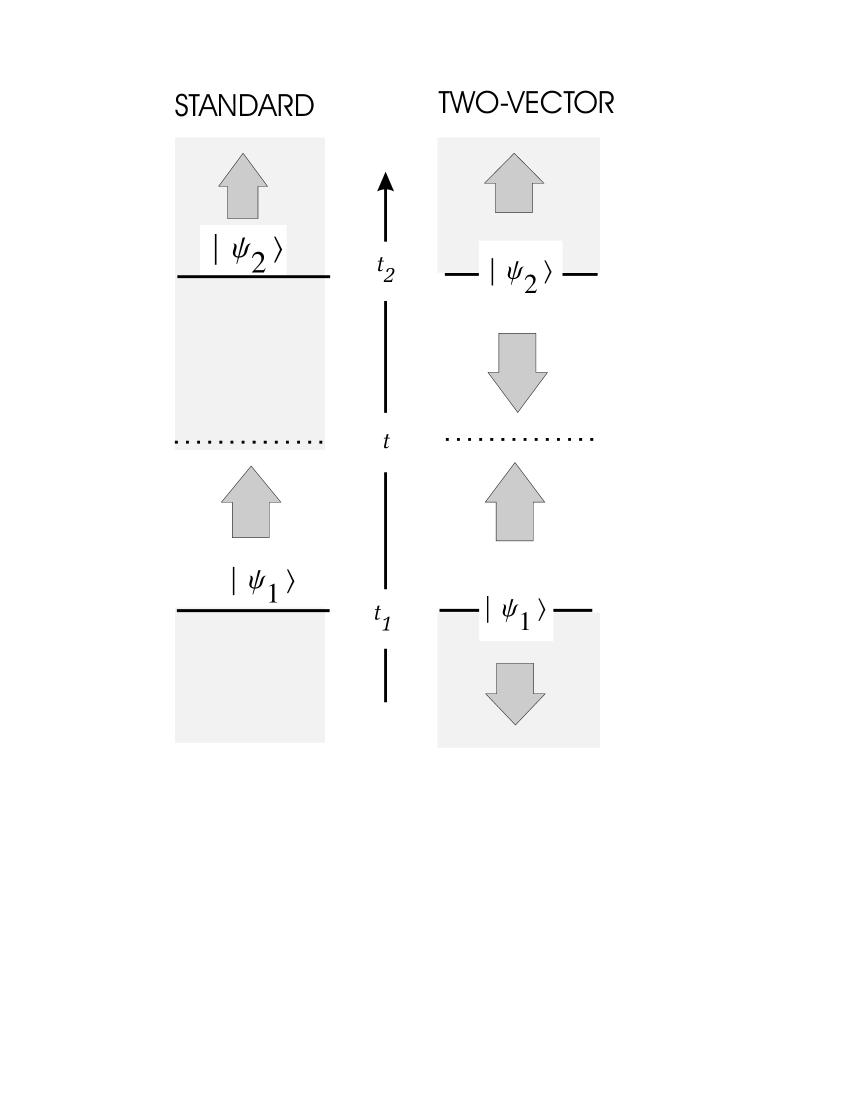
Figure 1.1: Description of the system at a time $t$ according to the Standard vs. the Two-Vector Formulations. The solid horizontal lines represent complete ideal measurements. The lightly shaded regions represent information that according to each of the formulations is irrelevant for the description of the system at the time $t$.

It seems therefore that in this formulation, it should indeed be possible to assign simultaneous properties to two non-commuting observables, for instance, in the case considered earlier of two successive measurements of $S_{x}$ and $S_{z}$, where $|\psi_{1};t\rangle$ corresponds to $``S_{x}=1/2"$, and $|\psi_{2};t\rangle$ to $``S_{z}=1/2"$. This however still leaves the question open as to how to give a non-trivial operational meaning to statements such as $``S_{x}=1/2$ and $S_{z}=1/2"$ at the intermediate time $t$.

One possibility is of course to consider ordinary ideal measurements of $S_{x}$ or $S_{z}$ that could have been performed at this intermediate time. In this sense, it is clear that given the two boundary conditions, had one also measured $S_{x}$ at time $t$ then the outcome certainly must have been $+1/2$. Similarly, had one measured $S_{z}$ instead, then the outcome must also have been $+1/2$, with certainty. But what about a joint measurement of $S_{x}$ and $S_{z}$? Or say a single measurement of the component $(\hat{S}_{x}+\hat{S}_{z})/\sqrt{2}$, which would seem to be well-defined except that the “inferred value” is the impossible value $1/\sqrt{2}$!

Such questions demand a closer examination into the actual dynamics of the measurement process and in particular the general notion that in quantum mechanics, a measurement is accompanied by a disturbance of the system. This notion may be argued from simple complementarity [2] arguments, which suggest how the conditions on the apparatus which define what is “ideal” about an ideal measurement –namely that they yield precise readings, entail conditions which are far from ideal from the point of view of the back-reaction effects on the system.

For concreteness, suppose one wishes to measure the spin component $S_{x}$ of an atom as in a Stern-Gerlach experiment, by imparting an impulse $\delta p=g\,S_{x}$ to the momentum $p$ along the $x$ direction (where $g$ is a coupling constant). This momentum plays the role of the “pointer variable” of the apparatus. An effective Hamiltonian describing the coupling between the two degrees of freedom is then $H=-g\delta(t)xS_{x}$, which simulates a brief passage of the atom through an inhomogeneous magnetic field with a linear gradient in the $x$ direction. This coupling, however, also describes a back-reaction effect on the spin, namely the precession of the angular momentum vector around the $x$-axis by an angle $\delta\theta=gx$. Now, as in an ideal measurement one would need to define $p$ to an accuracy $\Delta p\ll g$, then its complementary variable $x$ must be uncertain by an amount $\Delta x\gg g^{-1}$. This entails however that the uncertainty in the rotation angle is already $\Delta\theta\gg 1$, i.e., of an order greater that one complete revolution (see Fig. 1.2).

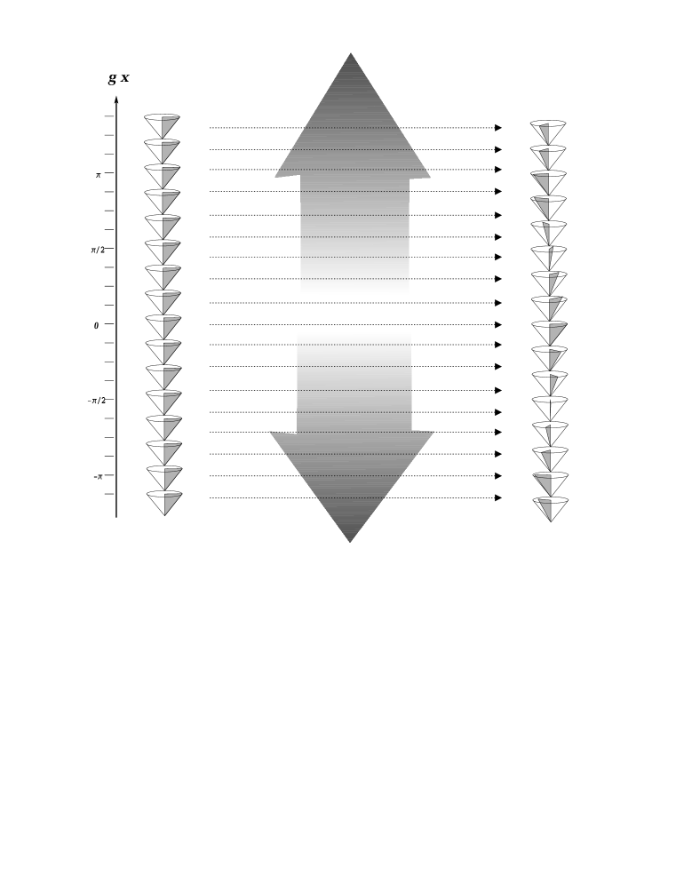
Figure 1.2: A classical picture of de-phasing in a Stern-Gerlach apparatus. The gradient in the magnetic field induces a differential rotation in the spin components perpendicular to the $x$ axis. If the uncertainty in $gx$ is of order $\pi$, this angular information is lost in the sample.

The argument illustrates therefore that the defining conditions of the apparatus necessary for an ideal measurement of a spin component simultaneously entail a de-phasing condition: the “washing out” of angular momentum information sensitive to a rotation around the measured spin axis. It seems therefore that in order to probe non-trivial aspects of quantum mechanics which may seem natural from the point of view of the two-vector description, one must resort to alternative intermediate measurement procedures where the connection between the two vectors is not broken by this de-phasing action of the apparatus.

It was this insight which lead the group of Aharonov to consider the scheme of weak measurements, from which the concept of weak values ultimately emerged. The weak measurement scheme differs from that of ideal measurements in that instead of controlling the apparatus “pointer variable” $p$ so as to ensure a precise reading in a single trial, it is now the dispersion $\Delta x$ in the complementary variable $x$ which one seeks to minimize so as to ensure a minimal back-reaction. Thus, for instance, the mutual disturbance entailed by a pair of measurements of two non-commuting observables may be controlled if one sacrifices the statistical significance of a single reading of the pointer variables. This cost is easily offset in the long-run; the systematic effects on the pointers may still be recovered when the weak measurement is performed independently on each member of large enough sample of similarly conditioned systems, i.e., as in a so called “precision measurement”.

Now, when developed within a purely quantum description, what the analysis of weak measurements revealed was the remarkable way in which the apparatus should respond systematically to those systems that happen to fulfill the initial and final conditions prescribed by the two vectors $|\psi_{1};t\rangle$ and $|\psi_{2};t\rangle$. For instance, if the initial and final states are such that $``S_{x}=1/2$ and $S_{z}=1/2"$ respectively, then indeed weak measurements of $(\hat{S}_{x}+\hat{S}_{z})/\sqrt{2}$ register the “impossible” value $1/\sqrt{2}$!  [8, 9] (Fig 1.3). More generally, on a sample of systems pre- and post-selected in the states $|\psi_{1};t\rangle$, and $|\psi_{2};t\rangle$ respectively, the average displacement of the pointer variable in a weak measurement of $\hat{A}$ is given by

$$\langle\delta p\rangle={\rm Re}A_{w}(t)$$ (1.5)

where $A_{w}(t)$ is the weak value of $\hat{A}$

$$A_{w}(t)=\frac{\langle\psi_{2};t|\hat{A}|\psi_{1};t\rangle}{\langle\psi_{2};t|\psi_{1};t\rangle}\,.$$ (1.6)

The imaginary part of $A_{w}(t)$ can also be related in the context of weak measurements to a change of order $\Delta x^{2}$ in the expectation value of the complementary variable $x$.

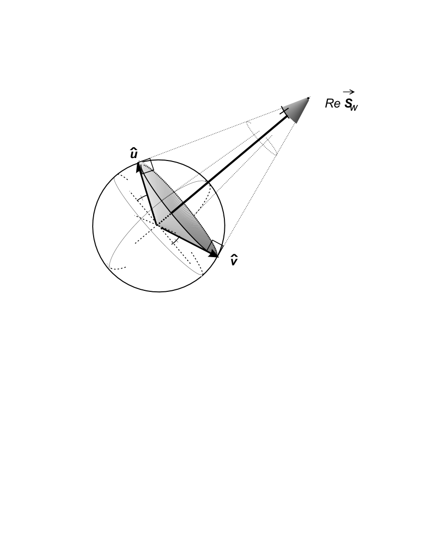
Figure 1.3: Geometry of Weak Values for a Spin-$1/2$ particle (real part shown only). The polarizations of the initial and final states are $\hat{u}$ and $\hat{v}$. The real part of the weak spin vector $\vec{S}_{w}$ bisects the angle between the two directions and its length is such that onto each of these directions the projection is $1/2$ (in units of $\hbar$). In a weak measurement of the spin component along some arbitrary direction $\hat{A}$, the average kick on the apparatus, from a sample satisfying the two boundary conditions, is then $\vec{S}_{w}\cdot\hat{a}$.

The most salient feature of the weak value is therefore that as opposed to the standard expectation value $\langle\psi_{1};t|\hat{A}|\psi_{1};t\rangle$, its real part may take values outside the spectrum of $\hat{A}$ if such spectrum is bounded [9, 10, 5]. Thus may follow any number of non-intuitive results if the weak value is viewed as some sort of “posterior average” of the eigenvalues of $\hat{A}$. Instead, in the context of weak measurements, weak values provide a new way of interpreting the standard expectation value. This is based on the fact that the small disturbance condition entails that the probability of a transition $|\langle\psi_{2};t|\psi_{1};t\rangle|^{2}$ between the initial and final state is practically unmodified by the presence of the measurement. The standard expectation value of $\hat{A}$, which is the observed mean value of $\langle\delta p\rangle$ on the pre-selected sample, can therefore be understood as an average of weak values:

$$\langle\psi_{1};t|\hat{A}|\psi_{1};t\rangle=\sum_{|\psi_{2};t\rangle}|\langle\psi_{2};t|\psi_{1};t\rangle|^{2}\times\frac{\langle\psi_{2};t|\hat{A}|\psi_{1};t\rangle}{\langle\psi_{2};t|\psi_{1};t\rangle}$$ (1.7)

where the sum runs over the final states defined by the post-selection. This sum rule shows that while in general the weak value will take values outside of the spectrum of $\hat{A}$, exceptionally large weak values are registered only under equally exceptional or unlikely conditions; in other words, the most likely weak values are still the ones falling within the ordinary range of expectation. But more importantly, the sum rule suggests that the weak value may be interpreted as a more basic definite property of the system, only that it is generally uncertain a priori, i.e., to the extent that the “destiny” of the system, as defined by the final state $|\psi_{2};t\rangle$, cannot be known in advance.

Returning then to the previously mentioned problem of inference posed by the standard interpretation, we thus see that the two vector-formulation, in conjunction with the scheme of weak measurements, suggests an attractive solution, the “twist” of which is lies in the separation between the measurement procedures by which the two concepts of “state” and “physical property” are to be defined operationally:

1. according to the two-vector formulation, the most basic ensemble to which the system may be assigned at a time $t$ is the pre- and post- selected ensemble defined by the outcome of two complete ideal measurements, which is is truly the maximal ensemble in the sense of both prediction and retrodiction. Such are the ensembles described by the two state vectors $|\psi_{1};t\rangle$ and $|\psi_{2};t\rangle$. The role of ideal measurements in establishing the connection between statistical ensembles and the concept of state is thus preserved as in the standard interpretation.

2. However, in contrast to the standard interpretation, the operational definition of the physical property associated with the observable $\hat{A}$ is to be grounded on weak measurements, i.e. from the weak value of $\hat{A}$ [14]. This presents no contradiction to the standard definition of $``A=a"$, when the initial state is an eigenstate of $\hat{A}$; in such cases the weak value is well-defined and coincides with the eigenvalue $a$. But since weak measurements hardly disturb the individual system, i.e., the state is not “collapsed”, the weak value retains its operational meaning even in the context in which other observables are measured weakly. It is this fact that allows weak values to be regarded as intrinsic properties of the system.

1.2 Statement of The Problem

The idea of formulating the model presented in this dissertation emerged from a question that has been troubling me for a couple of years:

In what sense can the weak value of $\hat{A}$ be interpreted as a definite mechanical effect of the system on the measuring apparatus?

This question was prompted by the fact that when the weak measurement scheme is analyzed quantum mechanically, it is also possible to view the unusual effects of weak values as something of a mathematical curiosity–an atypical way in which certain wave functions describing the apparatus, shifted by the eigenvalues of $\hat{A}$, happen to interfere so as to yield something that appears to be a “kick” of the apparatus pointer variable $p$ by the weak value. The impression of a “conspiracy in the errors” is only heightened by the fact that the statistics that show weak values are the ones where an additional final condition is controlled on the system, so it also legitimate to wonder whether at the level of probabilities, Bayes’ theorem plays a role in this conspiracy.

My first attempt at an answer was to look at these effects by drawing parallels with a classical Bayesian analysis of the measurement scheme. The result of this was that weak values could be interpreted as posterior averages of some quantity “$A$”, attached to the system, but only if one uses negative probabilities to account for the interference terms as in the Wigner representation. This however, turned the problem of interpreting weak values into the much more abstract problem of interpreting non-standard probabilities [12], and so I finally gave up on this route. Fortunately, two useful leads did come out of this parallel with the classical situation:

First came an awareness of the importance of the variable $x$ conjugate to the apparatus pointer variable $p$, which drives the reaction back on the system. As it turns out, when in the classical case one is interested in predicting the data, information about this variable is irrelevant. However, the variable becomes entirely relevant when the data is analyzed in retrospect, against initial and final boundary conditions on the system; prior knowledge of this variable then enters into our a posteriori inferences about both a) the state of the system that is sampled in a measurement and b) the state of the apparatus before the measurement started. This convinced me that there was something qualitatively important about looking at the measurement process given two boundary conditions on the system, as it is then when one expects the data to show an imprint of the back-reaction on the system entailed by the variable $x$.

Secondly, it also became obvious from the Bayesian analysis that what one calls an inference about the system in the measurement process is strictly tied to the underlying model one has for the data. What may then seem contradictory from the point of view of one model may be entirely plausible from the other. This lead me to suppose that perhaps the entirely different apparatus conditions for ideal and weak measurements entail, in parallel, qualitatively different dynamical conditions in the measurement interaction, and that in turn, these differences should be interpreted in terms of two different effective models for the data.

With the two above leads a general scenario emerged, which will be described in full in the coming chapter:

When the apparatus pointer-variable statistics are analyzed in the light of fixed initial and final (complete) boundary conditions, a clear distinction emerges between two ideal extremes depending on the initial preparation of the apparatus. Each extreme corresponds to a deliberate “control” on the part of the experimentalist aiming at optimizing either side of the disturbance vs. precision trade-off entailed by the uncertainty relations $\Delta x\Delta p\simeq 1/2$. Correlatively, it is possible to associate with each extreme a linear statistical model of the form

$$p_{f}=p_{i}+A$$ (1.8)

that describes the resultant conditional distribution of the data in terms of “kicks” proportional to $A$: in the case of sharp $p$, what we shall call the standard linear model (SLM), in which the “$A$” takes values on the spectrum of $\hat{A}$; in the case of sharp $x$, a weak linear model (WLM) in which “$A$” is the real part of the weak value $A_{w}$.

The fact that the two models are applicable in either extreme can be argued as a consequence of two different conditions by which it seems reasonable that the distribution of the data may be separated in terms of variables attached to the system or the apparatus respectively. In the “strong” extreme $\Delta p\rightarrow 0\Rightarrow\Delta x\rightarrow\infty$, these conditions can be tied to de-phasing, the loss of phase information in the data; in the weak extreme $\Delta x\rightarrow 0\Rightarrow\Delta p\rightarrow\infty$, the conditions can be tied to physical separability: the almost complete absence of entanglement between the system and the apparatus.

In between these two ideal extremes lies the “limbo” of non-ideal measurements where neither model is applicable; from within the perspective of the two above ideal extremes, this corresponds to the fact that neither has an effective de-phasing been achieved as required for the SLM analysis, nor has the necessary degree of “weakness” or physical separability been achieved as required for the WLM analysis. When viewed from this perspective, the “limbo” region should hence be of considerable interest when analyzed in the light of final boundary conditions as the non-separability of the conditional data may then be interpreted as the signature of the intrinsic quantum mechanical non-separability of the apparatus-system composite at the time of the measurement interaction.

For instance, it may seem reasonable to expect that in moving from one extreme to another within the parameter space of measurement strength, i.e., $\Delta x$, one should encounter in the limbo region an intermediate transition regime separating two regimes in each one of which the data is approximately captured by either of the two descriptions. One may then speculate that this transition in the description of the data is a signature of something analogous to a phase transition, an underlying qualitative change in the actual physics of the measurement interaction as one moves from one regime to the other in the strength parameter space.

Now, there is of course a way of describing the limbo region based on the probability amplitudes from which the conditional distributions of the data are ultimately derived. At present, however, the sense in which the interference patterns are understood is based on the spectral decomposition of $\hat{A}$. Such a description may be appropriate in a strong regime, where approximate statistical separability is possible under the SLM, but it fails to do justice to the overall qualitative behavior exhibited in the weak regime, where the mass of the resultant conditional distribution of the data may lie well outside the prior region of expectation.

What is missing therefore is a picture at the level of probability amplitudes that “sharpens” as the ideal conditions for statistical separability under the WLM are approached, in other words, that sharpens with the complementary variable $x$ of the apparatus.

1.3 Summary of Results

The aim of the model proposed in this dissertation is then to provide this complementary description. The idea is that the WLM, or a linear statistical model based on weak values, can be approached from the point of view of a quantum analog of a non-linear classical model in which a picture of “sampling” weak values is always at the forefront.

As we shall see in Chapter 3, it is possible to establish, by turning the emphasis towards the complementary variable $x$ of the apparatus, a clear criterion by which the real part of the weak value can be regarded as a definite kick of the pointer variable. This can be shown by considering narrow “sample” test functions of the apparatus in which the support in $x$ is bounded. In that case, the shift in the conjugate variable $p$ can be seen to be in direct correspondence with a phase gradient as in ordinary wave mechanics. Furthermore, by changing the location of the sample along $x$, the response of the pointer is given by different “local” weak values, each one corresponding to a different pair of initial and final states parameterized by $x$. Thus one obtains a picture where as the location of the test function is varied, one samples a different configuration of the system. The distribution of the data for an arbitrary apparatus preparation may then be understood as the resulting interference pattern when samples at various locations in $x$ are coherently superposed, what we call a superposition of weak measurements.

A more delicate question involves the interpretation, in the non-weak regime, of what in the weak regime corresponds to the imaginary part of the weak value. It is this component which in the model is associated with the Bayesian aspect.

The insight into this association is developed first in Chapter 4, where we consider the classical probabilistic analysis of the measurement with two boundary conditions on the system. This analysis shows how the posterior distribution of the classical pointer variable acquires a non-trivial dependence on the prior distribution in its conjugate variable $x$. This dependence has to do as mentioned earlier both with the region of the system’s phase space that is sampled, as well as with a re-assessment of the probabilities for possible initial conditions of the apparatus. This dependence is summarized in terms of what is known as a likelihood factor, which describes the passage from prior to a posterior probabilities given the conditions on the system.

From the classical analysis we then develop in Chapter $5$ the quantum analysis by drawing both on a formal correspondence as well as a quantitative correspondences that one should expect in the classical limit. The semi-classical analysis shows that the real part of the local weak value corresponds in the classical limit to the classical response of the apparatus given a definite value of $x$. Moreover, in the semi-classical analysis one can also establish for the quantum case, a direct correspondence with the classical likelihood factor. The model is then developed for more general boundary conditions by drawing a correspondence with the semi-classical case. The two elements of the model are then the local real part of the weak value, which is a non-linear function in $x$, and the likelihood factor. These two elements provide an intuitive way of understanding the two foremost statistics of the data, the mean and the variance. We obtain some new results in connection with such “error laws”.

Furthermore, the picture that emerges is that one samples different weak values, corresponding to different configurations of the system, but the a priori sampling weights are modified by the likelihood factor. The weak linear model is then recovered when the “sampling distribution” in $x$ is sharp enough that the uncertainty in the sampled weak values is small. In that case, the likelihood factor entails a small shift of the a priori distribution in $x$, which is then connected to the imaginary part of the complex weak value.

However, as the width in $x$ is increased, the likelihood factor produces qualitative changes in the sampling distribution. In Chapter $6$ we explore this phenomenon for those cases where an unlikely combination of boundary conditions yields “eccentric” weak values. Those cases can be connected to an interesting phenomenon in Fourier analysis known as super-oscillations, where the phase of a function oscillates in a certain interval more rapidly than any one of the component Fourier modes. However, as super-oscillations are exponentially suppressed in amplitude, this translates in the model to regions in $x$ where the likelihood factor is at a minimum or close to a minimum; the tendency of the likelihood factor is then to “widen” the sampling distribution. What happens then is that as the strength parameter $\Delta x$ is increased away from zero, at some critical value the sampling distribution shows a behavior analogous to a phase transition, where it goes from a single-peaked to a double-peaked function. In the reciprocal space of the pointer variable, the transition corresponds to the shift of the expectation value from the “eccentric” region to the normal region of expectation, accompanied by “beats”. We give an example where the beats are directly connected to the spectrum of the observable $\hat{A}$.

Chapter 2 Preliminaries: Standard and Weak Linear Models

In this chapter we introduce the general setting in which we would like to place our non-linear Bayesian model of non-ideal measurements. Associated to any measurement scheme is a some statistical model–a constraint equation allowing us to connect the data to the properties that are to be inferred from the measurement. The well-known von-Neumann [18] measurement scheme is perhaps the simplest caricature of a measurement interaction and leads to the simplest possible model: the linear model. It turns out that this model, which we shall henceforth refer to as the standard linear model, is consistent with quantum mechanical predictions to the extent that the statistics are analyzed against initial conditions only; moreover it is consistent under very general non-ideal conditions on the apparatus. However, the model may fail when the statistics are controlled for the most restrictive type of conditions that can be imposed on the measured system, namely initial and final conditions. It is this failure that gives room to the unexpected effects associated with weak values, and which suggests that an alternative interpretation of the data may be in order.

2.1 The von Neumann Scheme

The von Neumann measurement scheme consists of an interaction between two initially unentangled systems, the “system” proper and an external apparatus. The aim of this interaction is to produce an effect on the apparatus from which to infer the value of some observable $\hat{A}$ of the system. The distinction between the two systems follows from the underlying assumption that the “system” is generally microscopic while the apparatus is either macroscopic, or else satisfies certain classical properties expected of a macroscopic object, in which case the measurement is called an indirect measurement. One such property is for instance that the mass be large enough that quantum inertial effects (i.e., wave-packet spreading) can be neglected on the side of the apparatus, at least for the duration of the measurement interaction. The apparatus is then idealized as a system of infinite mass with a vanishing free Hamiltonian, described by a pair of canonically conjugate variables $\hat{x}$, $\hat{p}$, ($[\hat{x},\hat{p}]=i$). We distinguish the variable $\hat{p}$ as the pointer variable, the observable on which the effect is analyzed and from which the datum is ultimately obtained. In addition, we shall also refer to the conjugate variable $x$ as the reaction variable, for resons that will become evident shortly.

The simplest dynamical model of a von-Neumann interaction is described by the impulsive Hamiltonian operator

$$\hat{H}_{M}(t)=-\delta(t-t_{i})\hat{A}\ \hat{x}\,,$$ (2.1)

coupling $\hat{A}$ to the reaction variable $x$, where the delta-function models the fact that the interaction time is negligible compared to that of the free evolution of the system. What distinguishes this type of coupling is that the impulsive unitary operator

$$\exp(-i\int dt\,H_{M}(t))=e^{i\hat{A}\hat{x}}$$ (2.2)

which is therefore defined induces in the Heisenberg picture a linear transformation of the pointer variable operator

$$\hat{p}_{f}=e^{-i\hat{A}x}\,\hat{p}_{i}\,e^{i\hat{A}x}=\hat{p}_{i}+\hat{A}\,.$$ (2.3)

Were one to drop the hats, this equation would be interpreted classically as a “kick” of the pointer variable proportional to the value of “$A$”. In such case, the value of “$A$” could then be inferred from the impulse imparted to the apparatus.

The archetype of such scheme is provided by the Stern-Gerlach apparatus (see Fig. 2.1), in which case $\hat{A}$ stands for a given spin component, i.e., $\hat{S}_{x}$, and $\hat{x}$ stands for the translational coordinate of the particle along the direction parallel to the spin component. The spin component is then determined from the asymptotic deflection of the particle which in the limit $t\rightarrow\infty$ is proportional to the imparted impulse. We should note that a possible coupling constant, which for instance in the S-G device would involve the product of the gyromagnetic factor and the magnetic field gradient, can always be absorbed in a canonical redefinition of $\hat{x}$ and $\hat{p}$. Other examples of such linear von-Neumann setups can be found in  [19].

Now, the conditions under which the above classical analysis of the datum can be performed in a single realization of the measurement correspond to what we shall henceforth refer to as a strong measurement, or what is commonly known as the “ideal” realization of the measurement. This means that the initial state of the apparatus is sufficiently well-defined in $p$ that the value of “$A$” can be inferred precisely from the displacement $\delta p=p_{f}-p_{i}$. As is well known, the possible “kicks” are then the eigenvalues $\{a\}$ of $\hat{A}$, which occur with probability

$$P(a|\hat{\rho}_{s})=Tr[\hat{\Pi}(a)\,\rho_{s}]$$ (2.4)

where $\hat{\Pi}(a)$ is the projection operator onto the corresponding eigenspace and $\rho_{s}$ is the density matrix describing the initial preparation of the system).

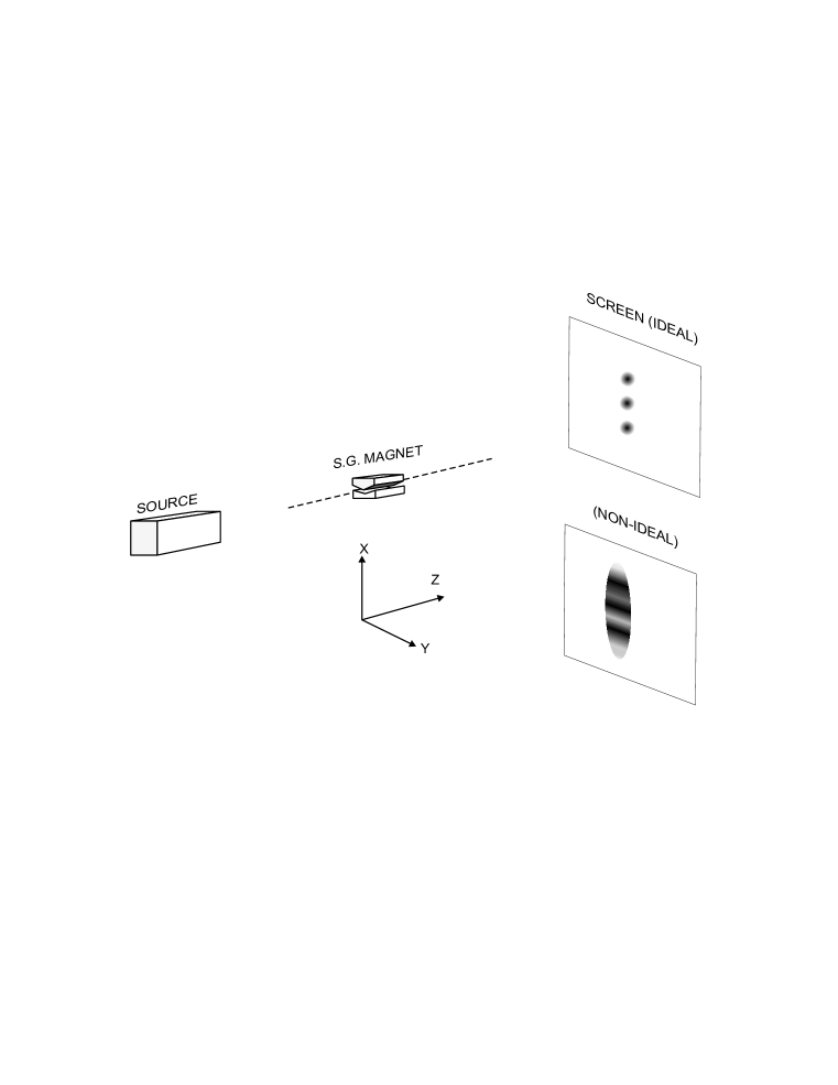
Figure 2.1: Schematic of a Stern-Gerlach apparatus for the measurement of a spin component, in this case illustrating the measurement of the $S_{x}$-component of a spin-$1$ particle. Directions of spin not perpendicular to the beam path may be measured by passing the beam through a uniform magnetic field oriented in such a way so as to produce a desired rotation of the spin axis relative to the measured axis. The data is obtained from the vertical position of the spot on the screen. In the ideal case, only three spots are seen, always aligned with the direction of the S-G magnet. In the non-ideal realization illustrated here, the dispersion in the data is so large that the eigenvalues are barely distinguishable.

2.2 The Standard Linear Model

In more realistic “non-ideal” situations, the initial state of the apparatus will have a finite and perhaps considerable dispersion in $p$. Strictly speaking then, the classical picture of “kicks” proportional to the eigenvalues of $\hat{A}$ should no longer be applicable. However, it is easily shown that if the initial states of the system and apparatus are physically separable, i.e., no entanglement, then even in less than ideal circumstances, the predicted distribution of the data is still statistically separable under the c-number linear model

$$p_{f}=p_{i}+a\,,$$ (2.5)

which we shall here refer to as the “standard linear model” or SLM for short, in which $p_{f}$ is the datum, $p_{i}$ plays a role analogous to the “noise”, and the “signal” $a$ –the target of inference– takes values on the eigenvalues of $\hat{A}$. By statistical separability we shall mean that the resultant distribution of the data can be decomposed, in terms of a number of additional conditions, so that $p_{i}$ and $a$ can be treated at some level as if they were independent random variables, in this case attached to the apparatus and the system respectively.

Consistency of the predicted distributions with the SLM follows from the equivalence between the Heisenberg and Schrödinger pictures and the assumption of physical separability. To see this, consider first the case we shall keep in mind throughout this dissertation, that of a pure preparation in which the system and apparatus are prepared in a factorable state $|\Psi_{i}\rangle=|\psi_{1}\rangle\otimes|\phi_{i}\rangle$ where $|\psi_{1}\rangle$ is the initial state of the system. With the measurement interaction, $|\Psi_{i}\rangle$ undergoes the transformation

$$|\Psi_{i}\rangle=|\psi_{1}\rangle\otimes|\phi_{i}\rangle\rightarrow|\Psi_{f}\rangle=e^{i\hat{A}\hat{x}}|\Psi_{i}\rangle\,.$$ (2.6)

The probability distribution for the data is then

$$dP(p\,|\Psi_{f})=dp\,\langle\Psi_{f}|\delta(p-\hat{p})|\Psi_{f}\rangle\,.$$ (2.7)

Now use the Heisenberg picture transformation (2.3) and the spectral resolution of $\hat{A}$ to obtain

$$dP(p\,|\Psi_{f}) = dp\,\langle\Psi_{i}|e^{-i\hat{A}\hat{x}}\delta(p-\hat{p})e^{i\hat{A}\hat{x}}|\Psi_{i}\rangle$$ (2.8)

$$= dp\,\langle\Psi_{i}|\delta(p-\hat{p}-\hat{A})|\Psi_{i}\rangle$$

$$= \,\sum_{a}\langle\psi_{1}|\hat{\Pi}(a)|\psi_{1}\rangle\ dp\langle\phi_{i}|\delta(p-\hat{p}-a)|\phi_{i}\rangle$$

$$= \sum_{a}P(a|\psi_{1})\,dP(p-a\,|\phi_{i})\,.$$

From this equation we observe that the distribution of the data takes the form of a “broadened” version of the spectral distribution $P(a|\psi_{1})$– the convolution of $P(a|\psi_{1})$ with a probability distribution for the “noise” $dP(p|\phi_{i})$. To illustrate this, we show in Fig. 2.2 the resultant distribution for a spin-$1$ measurement with three values of the uncertainty in $p$. Fig. 2.3 then shows how in the non-ideal cases, where the peaks of the spectrum are not resolved, it is still possible to view the distribuition as a sum of broadened spectral distributions.

It is this form which underlies the fact that even if the uncertainty in the noise is large but its probability distribution is known, then after a large number of independent and identical realizations of the measurement one may still determine properties of the spectral distribution from the observed frequency distribution of the data. For instance, if we know the initial mean value $\langle p\rangle_{i}$ of the pointer variable and its variance $\Delta p_{i}^{2}$, we may then use the “error” formulas which stem from the SLM

$$\langle p\rangle_{f} = \langle p\rangle_{i}+\langle a\rangle$$

$$\Delta p_{f}^{2} = \Delta p_{i}^{2}+\Delta a^{2}$$ (2.9)

to connect the observed means and variances in the data with the standard expectation value of $\hat{A}$ and its variance

$$\langle a\rangle = \sum_{a}P(a|\psi_{1})\,a=\langle\psi_{1}|\hat{A}|\psi_{1}\rangle$$

$$\Delta a^{2} = \sum_{a}P(a|\psi_{1})\,(a-\langle a\rangle)^{2}=\langle\psi_{1}|\hat{A}^{2}|\psi_{1}\rangle-\langle\psi_{1}|\hat{A}|\psi_{1}\rangle^{2}\,.$$ (2.10)

More generally, the spectral distribution can be extracted by performing a deconvolution on the frequency distribution of the data (although for noisy data the problem is not entirely without complications, see e.g.,  [13]).

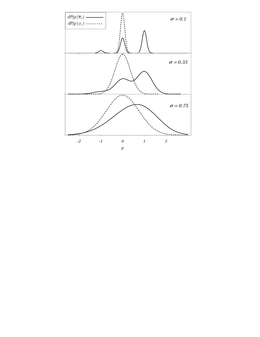
Figure 2.2: Pointer variable probability distributions for three values of the “noise” level in the apparatus preparation. In the three cases, the system is a spin-1 particle prepared in an eigenstate $|s=1,m_{s}=1\rangle$ of $\hat{S}_{z}$; The measurement is of the spin component $\hat{S}_{u}$, along a direction $\vec{u}=\sin(\pi/3)\vec{e}_{x}+\cos(\pi/3)\vec{e}_{z}$; the apparatus initial state is a minimum uncertainy packet with a standard deviation $\sigma$ in $p$ initially centered at $p=0$. The case $\sigma=0.1$ illustrates the ideal situation in which the spectrum of $S_{u}$ is clearly distibguished.

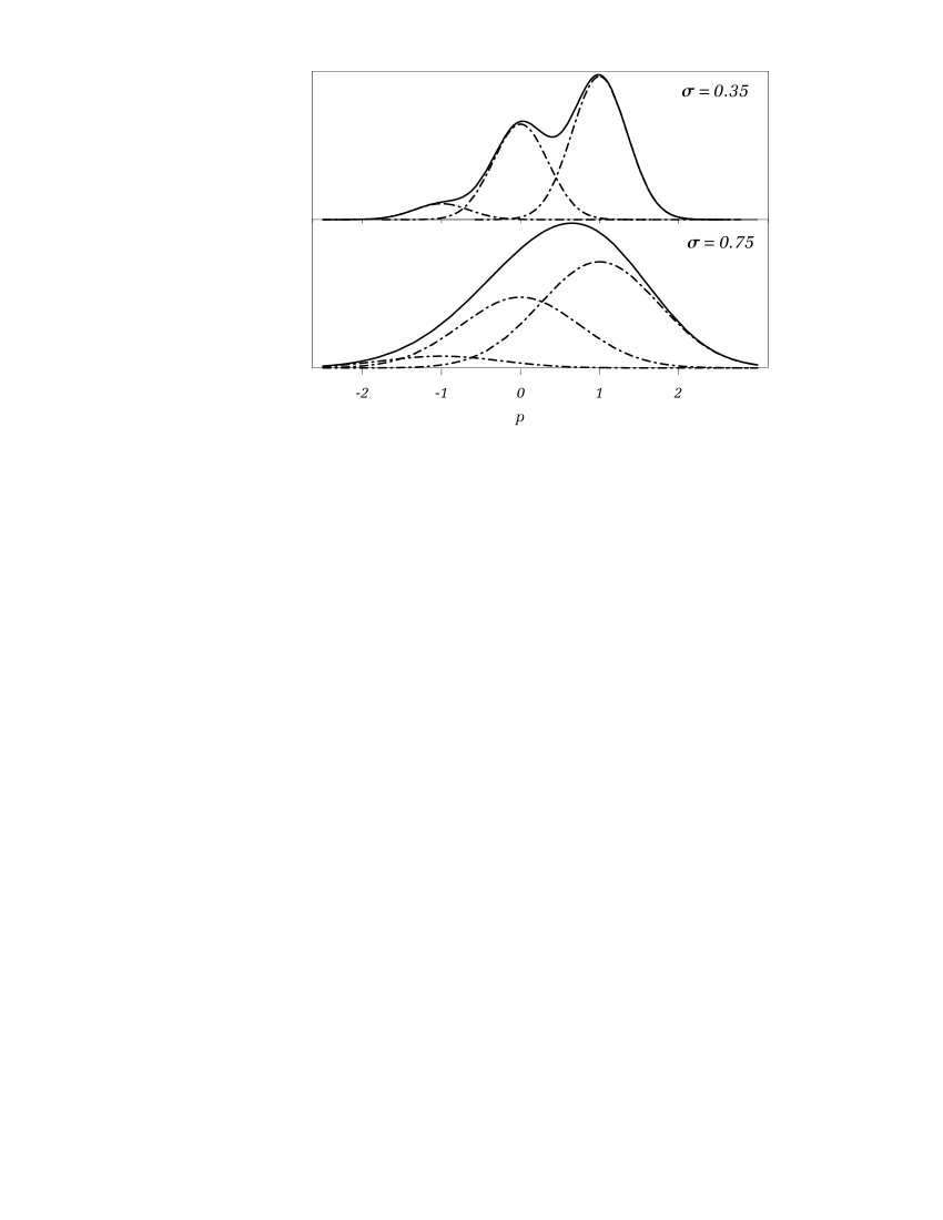
Figure 2.3: Break-up of the non-ideal distributions in Fig. 2.2 as a mixture of broadened spectral distributions. The spectral probabilities $\langle s=1,m_{z}=1|\hat{\Pi}(m_{u})|s=1,m_{z}=1\rangle$ are $1/16,\,3/8\,,9/16$ for $m_{u}=-1,0,1$ respectively. These probabilities correspond to the areas under the three peaks in the ideal situation $\sigma=0.1$. In all three cases the expectation value of $p$ over $dP(p|\Psi_{f})$ is $\frac{1}{2}$ and the variance is $\sigma^{2}$ plus the variance of the spectral distribution, $\sigma_{m}^{2}=3/8$.

Another equally instructive way of seeing the consistency of the SLM is by expanding the combined state initial state $|\Psi_{i}\rangle$ in an eigenbasis of $\hat{A}$, i.e.,

$$|\Psi_{i}\rangle=\left[\sum_{a,g}\langle a,g|\psi_{1}\rangle|a,g\rangle\right]\otimes|\phi_{i}\rangle$$ (2.11)

where $g$ stands for some additional degeneracy index. The combined final state may then be written as

$$|\Psi_{f}\rangle=\sum_{a,g}\langle a,g|\psi_{1}\rangle|a,g\rangle\otimes|e^{ia\hat{x}}\phi_{i}\rangle$$ (2.12)

where $|e^{ia\hat{x}}\phi_{i}\rangle$ is $|\phi_{i}\rangle$ shifted in $p$ by $a$. The distribution of the data can then be obtained from the resultant partial density matrix of the apparatus which is obtained by “tracing out” the states of the system from the projector $|\Psi_{f}\rangle\langle\Psi_{f}|$. Using the orthogonality of the basis $\{|a,g\rangle\}$, one then finds

$$\hat{\rho}_{a}(\Psi_{f}) = \sum_{a,g}\|\ \langle a,g|\psi_{1}\rangle\ \|^{2}\ |e^{ia\hat{x}}\phi_{i}\rangle\langle e^{ia\hat{x}}\phi_{i}|$$ (2.13)

$$= \sum_{a}P(a|\psi)\ |e^{ia\hat{x}}\phi_{i}\rangle\langle e^{ia\hat{x}}\phi_{i}|\,.$$

The partial density matrix describes therefore a mixture of shifted states. This mixture could have been generated, for instance, by applying unitary transformations $e^{ia\hat{x}}$ on the initial state of the apparatus, where the momentum shifts corresponded to some external random parameter $a$ distributed according to the probabilities $P(a|\psi)$.

Finally, we note that statistical separability under the SLM ensues in the more general case is which the two systems are prepared in a mixed and classically correlated separable state of the form

$$\hat{\rho}_{i}=\sum_{\chi}P(\chi|E)\,\hat{\rho}_{s}(\chi)\otimes\hat{\rho}_{a}(\chi)$$ (2.14)

where $\chi$ may be some external uncertain classical parameter. The predicted distribution of the data may then be decomposed as

$$dP(p\,|\rho_{f})=\sum_{\chi}P(\chi|E)\sum_{a}P(a|\rho_{s}(\chi))\,dP(p-a\,|\rho_{a}(\chi))\,,$$ (2.15)

which is nothing more than a statistical mixture of broadened spectral distributions.

Thus we see that in a von-Neumann linear measurement, and insofar as the combined initial state of the two systems is not entangled, the predicted distribution of the data is statistically separable under the SLM, i.e., a linear statistical model in which the “signal” takes values on the eigenvalues of $\hat{A}$. It may be tempting therefore to interpret this consistency as an indication of a wider range of validity of the classical dynamical picture $p_{f}=p_{i}+a$ underlying the SLM –in other words, that even when the spectrum is not fully resolved it is still assumed that on every realization of the measurement the pointer variable suffers a definite (i.e. “real”) “kick” $a\in Spec(\hat{A})$, except that the values of $p_{i}$ and $a$ fluctuate statistically on a trial-by-trial basis.

However, as we shall see shortly, it is indeed possible to distinguish certain populations of the system from which the distribution of the data is inconsistent with the SLM, and hence with the underlying physical picture. These are populations that are singled out according to additional conditions that the system may be made to satisfy after the measurement interaction, conditions which define the so-called pre-and post-selected ensembles mentioned in the introduction. We digress momentarily to develop the appropriate notation we shall use when dealing with such ensembles.

2.3 Description of the Post-Selected Statistics in Terms of Relative States

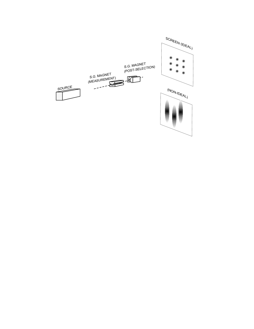
Figure 2.4: Schematic of a Stern-Gerlach setup with a post-selection. The second magnet splits the beam into three additional components, here corresponding to three eigenstates of $\hat{S}_{y}$. A post-selected sample for the first measurement corresponds to the set of all those events which fall into any one of the three distinct regions along the $y$ direction produced by the third measurement. Note that since $x$ and $y$ directions are perpendicular, the respective sets of canonical variables $(x,p_{x})$ and $(y,p_{y})$ commute; hence, if these two translational degrees of freedom are initially uncorrelated, the two magnets implement independent measurements.

Let us then suppose that after our von-Neumann measurement of $\hat{A}$, a second complete ideal measurement is performed independently on the system, the possible outcomes of which correspond to a complete orthonormal set of final states $\{|\psi_{\mu}\rangle\}$ with $\langle\psi_{\mu}|\psi_{\nu}\rangle=\delta_{\mu\nu}$ and $1_{s}=\sum_{\mu}|\psi_{\mu}\rangle\langle\psi_{\mu}|$. An example of how such a post-selection may be implemented for a Spin-$1$ particle is given in Fig. 2.4. Together with the fixed initial state $|\psi_{1}\rangle$, each $|\psi_{\mu}\rangle$ defines a pre-and post selected ensemble for the system that will be labeled throughout this dissertation by the index $\mu$. We shall generally refer to such ensemble simply as a “transition” $|\psi_{1}\rangle\rightarrow|\psi_{\mu}\rangle$, where it should always be understood that since in the interim time the system interacted with our apparatus, transition probabilities are not necessarily $|\langle\psi_{\mu}|\psi_{1}\rangle|^{2}$; instead they are given by

$$P(\psi_{\mu}|\Psi_{f})=\langle\Psi_{f}|\ |\psi_{\mu}\rangle\langle\psi_{\mu}|\ |\Psi_{f}\rangle\,,$$ (2.16)

which we denote as the perturbed transition probabilities. Finally, and for simplicity, unless otherwise noted, we henceforth use the terms “conditional” and “unconditional” in the sense of conditioning or not against the final outcome $|\psi_{\mu}\rangle$ of the post-selection.

Now, referring to the states $|\Psi_{i}\rangle$ and $|\Psi_{f}\rangle$ of Eq. (2.6), a convenient way of keeping track of both the conditional and unconditional statistics is by means of the relative-state expansion of the combined final state $|\Psi_{f}\rangle$ defined by the final basis:

$$|\Psi_{f}\rangle=\sum_{\mu}\,\sqrt{P(\psi_{\mu}|\Psi_{f})}\ |\psi_{\mu}\rangle\otimes|\phi_{f}^{(\mu)}\rangle\,,$$ (2.17)

where $|\phi_{f}^{(\mu)}\rangle$ is the state of the apparatus relative to the final outcome $|\psi_{\mu}\rangle$

$$|\phi_{f}^{(\mu)}\rangle=\frac{1}{\sqrt{P(\psi_{\mu}|\Psi_{f})}}\ \ \langle\psi_{\mu}|e^{i\hat{A}\hat{x}}|\psi_{1}\rangle\,|\phi_{i}\rangle\,.$$ (2.18)

Note that $P(\psi_{\mu}|\Psi_{f})$ can be obtained from the normalization condition of this state. The relative state $|\phi_{f}^{(\mu)}\rangle$ encodes all the available statistical information about the apparatus, conditional on the specific transition $|\psi_{1}\rangle\rightarrow|\psi_{\mu}\rangle$.

In turn, to obtain the unconditional statistics, one may take the partial trace of $|\Psi_{f}\rangle\langle\Psi_{f}|$ to obtain an alternative decomposition of the partial density matrix of the apparatus

$$\rho_{a}(\Psi_{f})=\sum_{\mu}P(\psi_{\mu}|\Psi_{f})\ |\phi_{f}^{(\mu)}\rangle\langle\phi_{f}^{(\mu)}|\,.$$ (2.19)

That this decomposition should yield the same density matrix as the one described by equation (2.13) is a good illustration of the fact that the break-up of a mixed state into a convex sum of pure states is not unique. What is, however, unique about this particular decomposition is that the components of the mixture can be distinguished a posteriori, in the sense that the corresponding statistics can be analyzed separately, using the information provided by the post-selection.

2.4 Failure of the SLM Under Both Initial and Final Conditions

Let us now consider the conditional probability distribution of the data which follows from a given relative state $|\phi_{f}^{(\mu)}\rangle$ as given in Eq. 2.18. Resolving $\hat{A}$, we see that $|\phi_{f}^{(\mu)}\rangle$ expands as a linear combination of momentum shifts of the initial state $|\phi_{i}\rangle$

$$|\phi_{f}^{(\mu)}\rangle=\frac{1}{\sqrt{P(\psi_{\mu}|\Psi_{f})}}\sum_{a}\langle\psi_{\mu}|\hat{\Pi}(a)|\psi_{1}\rangle\,|e^{ia\hat{x}}\phi_{i}\rangle\,,$$ (2.20)

each shift proportional to one of the eigenvalues. This defines therefore a relative wave function in the $p$ representation which is a coherent superposition of shifted wave functions weighted by generally complex coefficients

$$\phi_{f}^{(\mu)}(p)\propto\sum_{a}\langle\psi_{\mu}|\hat{\Pi}(a)|\psi_{1}\rangle\,\phi_{f}^{(\mu)}(p-a)\,.$$ (2.21)

The conditional distribution of the data, i.e., $dP(p\,|\phi_{f}^{(\mu)})=dp|\langle p|\phi_{f}^{(\mu)}\rangle|^{2}$, may thus be written as:

$$dP(p\,|\phi_{f}^{(\mu)})=\frac{dp\,\left|\sum_{a}\langle\psi_{\mu}|\hat{\Pi}(a)|\psi_{1}\rangle\,\phi_{i}(p-a)\right|^{2}}{\int dp^{\prime}\,\left|\sum_{a^{\prime}}\langle\psi_{\mu}|\hat{\Pi}(a^{\prime})|\psi_{1}\rangle\,\phi_{i}(p^{\prime}-a^{\prime})\right|^{2}}\,,$$ (2.22)

where the normalization constant in the denominator is a re-expression of the perturbed transition probability $P(\psi_{\mu}|\Psi_{f})$.

From the form of Eq. (2.22) we can immediately see that the presence of interference terms of the form

$$\langle\psi_{\mu}|\hat{\Pi}(a)|\psi_{1}\rangle\langle\psi_{1}|\hat{\Pi}(a^{\prime})|\psi_{\mu}\rangle\phi_{i}(p-a)\phi_{i}^{*}(p-a^{\prime})\ \ \ (a\neq a^{\prime})$$ (2.23)

prevents us from reducing this equation to either the statistically separable forms of a convolution of a probability distribution in $p$ and a probability distribution of the eigenvalues, as in Eq. (2.8), or to a mixture of such forms as in Eq. (2.15). This means therefore that the conditional distributions arising from the post-selected subsamples are generally not consistent with the standard linear model.

Aside from the trivial case in which either $|\psi_{1}\rangle$ or the $|\psi_{\mu}\rangle$ are eigenstates of $\hat{A}$, the notable exception is when the no overlap condition

$$\phi_{i}(p-a)\phi_{i}(p-a^{\prime})\simeq 0$$ (2.24)

is satisfied. In this case, the conditional distributions do reduce to the separable form

$$dP(p|\phi_{f}^{(\mu)})=\sum_{a}P(a|\psi_{1}\psi_{\mu})\,dP(p-a|\phi_{i})\,\,,$$ (2.25)

where $P(a|\psi_{1}\psi_{\mu})$ is the conditional distribution

$$P(a|\psi_{1}\psi_{\mu})=\frac{|\langle\psi_{\mu}|\hat{\Pi}(a)|\psi_{1}\rangle|^{2}}{\sum_{a^{\prime}}|\langle\psi_{\mu}|\hat{\Pi}(a^{\prime})|\psi_{1}\rangle|^{2}}\ \,,$$ (2.26)

presented in the introduction. The no overlap condition is of course the condition for the strong or “ideal” measurement where as mentioned previously the dynamical picture underlying the SLM is strictly applicable.

On the other hand, if $\phi_{i}(p)$ is wide enough that the interference terms become relevant in (Eq. 2.22), the dynamical picture $p_{f}=p_{i}+a$ is clearly inappropriate. As we show in Fig. (2.5) for the same example considered in Fig. (2.3), the discrepancies may be quite dramatic. For instance, if the spectrum of $\hat{A}$ is bounded spectrum, the central mass of the conditional distribution may lie outside the region of expectation defined by the SLM.

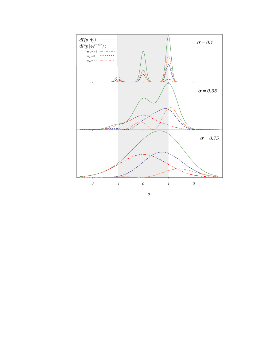
Figure 2.5: Posterior breakup of the unconditional distributions $dP(p|\Psi_{f})$ in Fig. 2.2, according to the results of a postselecting measurement of $\hat{S}_{v}$, where $\vec{v}=\sin(2\pi/3)\vec{e}_{x}+\cos(2\pi/3)\vec{e}_{z}$. Two manifestation of interference effects in the conditional distributions are a small bump at $p\simeq-1.3$ for $m_{v}=0$, $\sigma=0.35$ and, more notoriously, that the lower quartile of the $m_{v}=1$, $\sigma=0.75$ distribution lies approximately at the upper boundary of this “allowed” region $[-1,1]$.

What is interesting is that even in those cases we must nevertheless recover the separable form consistent with the dynamical SLM picture in the process of pooling the data from all the post-selected subsamples (this is also illustrated in Fig. 2.5). This is a consequence of the equivalence between the decompositions (2.19) and (2.13) of the partial density matrix $\rho_{a}(\Psi_{f})$ from which the unconditional data is obtained, which in particular entails the sum rule for the data

$$\sum_{\mu}P(\psi_{\mu}|\Psi_{f})\,dP(p\,|\phi_{f}^{(\mu)})=dP(p|\Psi_{f})\,.$$ (2.27)

This sum rule hides something of a “statistical decoherence” in the process of pooling of the data: substituting in Eq. (2.22) and noting that its denominator is the perturbed transition probability $P(\psi_{\mu}|\Psi_{f})$, we see that

$$\sum_{\mu}P(\psi_{\mu}|\Psi_{f})\,dP(p\,|\phi_{f}^{(\mu)})$$ (2.28)

may be written as

$$\sum_{\mu}dp\,\left|\sum_{a}\langle\psi_{\mu}|\hat{\Pi}(a)|\psi_{1}\rangle\,\phi_{i}(p-a)\right|^{2}$$

$$= \sum_{\mu}dp\,\sum_{a}\sum_{a}^{\prime}\langle\psi_{1}|\hat{\Pi}(a^{\prime})|\psi_{\mu}\rangle\langle\psi_{\mu}|\hat{\Pi}(a)|\psi_{1}\rangle\,\phi_{i}(p-a)\phi_{i}^{*}(p-a^{\prime})$$

$$= dp\,\sum_{a}\sum_{a}^{\prime}\langle\psi_{1}|\hat{\Pi}(a^{\prime})\sum_{\mu}|\psi_{\mu}\rangle\langle\psi_{\mu}|\hat{\Pi}(a)|\psi_{1}\rangle\,\phi_{i}(p-a)\phi_{i}^{*}(p-a^{\prime})\,;$$

now, using the completeness of the final basis $\sum_{\mu}|\psi_{\mu}\rangle\langle\psi_{\mu}|=1$, and the completeness of the projection operators $\hat{\Pi}_{a}\hat{\Pi}_{a}^{\prime}=\delta_{a,a^{\prime}}\hat{\Pi}_{a}$, this reduces to

$$dp\,\sum_{a}\sum_{a}^{\prime}\langle\psi_{1}|\hat{\Pi}(a^{\prime})\hat{\Pi}(a)|\psi_{1}\rangle\,\phi_{i}(p-a)\phi_{i}^{*}(p-a^{\prime})$$ (2.29)

$$= dp\,\sum_{a}\langle\psi_{1}|\hat{\Pi}(a)|\psi_{1}\rangle\,|\phi_{i}(p-a)|^{2}$$

$$= \,\sum_{a}P(a|\psi_{1})dP(p-a|\phi_{i})\,.$$

Thus we see that the interference terms in the conditional distributions add up to zero leaving only the incoherent terms, which are the ones yielding the separable form of Eq. (2.8) consistent with the SLM.

We should note then the non-trivial significance of the cancellations behind the sum rule (2.27): given the actual sequence of events of first reading the datum and then post-selecting, any features arising from the interference terms in the conditional distributions will be statistically indistinguishable a priori–against the background of the SLM-consistent unconditional distribution of the data $dP(p|\Psi_{f})$. Thus, discrepancies with the naive dynamical picture underlying the SLM are most definitely not obvious. They are only revealed a posteriori–here in the literal chronological sense–after binning the data using the trial-by-trial record of correlations between the readings and the outcome of the post-selection.

2.5 Weak Measurements and Weak Values

As mentioned in the introduction, in a weak measurement we seek to minimize the back-reaction on the measured system. It is easily seen from the measurement Hamiltonian (2.1) that this reaction is dictated by the variable $x$ conjugate to the pointer variable; for instance, following the Heisenberg dynamics on the side of the system, one can see that an arbitrary observable $\hat{B}$ of the system is transformed as

$$\hat{B}_{f}=e^{-i\hat{A}x}\hat{B}_{i}e^{i\hat{A}x}\,.$$ (2.30)

The aim is therefore to ensure that the dispersion in $x$ should be small around $x=0$ so that if $\hat{B}$ is sensitive ( $[\hat{B},\hat{A}]\neq 0)$, then $\hat{B}_{f}\simeq\hat{B}_{i}$.

This aim may also be seen from the point of view of entanglement. As one can see, if the initial state of the apparatus $|\phi_{i}\rangle$ were a “perfect” eigenstate of $x$, i.e. $|\phi_{i}\rangle=|x=0\rangle$, then the measurement transformation (Eq. 2.6) would leave the initial factorable state $|\Psi_{i}\rangle=|\psi_{1}\rangle\otimes|x=0\rangle$ state unchanged. Thus, one may view the minimal dispersion condition as being close to the ideal situation in which the initial physical separability or no entanglement between system and apparatus is preserved.

Now, as this aim can only be accomplished in general at the price of spreading the distributions in the conjugate variable $p$, the remarks made in the previous sections should then serve to underscore the relevance of the two boundary conditions in the statistical analysis of weak measurements. To wit, the unconditional distribution of the data from a pre-selected sample will show no unusual deviations from the SLM picture; it will only appear as a highly broadened spectral distribution. On the other hand, we should expect a considerable overlap between the shifted wave functions in the conditional distributions (2.22) of the post-selected sub-samples, and hence “hidden” deviations from the SLM dynamical picture.

What is interesting is that from these complicated interference effects a simple picture emerges, whereby the conditional statistics appear to reflect a single, well-defined “kick”, proportional to the real part of the weak value of $\hat{A}$, defined as

$$A_{w}^{(\mu)}=\frac{\langle\psi_{\mu}|\hat{A}|\psi_{1}\rangle}{\langle\psi_{\mu}|\psi_{1}\rangle}\,.$$ (2.31)

It was this fact, in conjunction with the defining conditions of weak measurements, which prompted the group of Aharonov and collaborators to propose that the weak value is an appropriate operational description of a system in between two ideal complete measurements. As in part the purpose of this dissertation is to provide a firmer grasp on the concepts of weak measurements and weak values, we shall here only give a cursory look at how weak values were originally derived and some of the unusual properties associated with them.

Aharonov, Albert and Vaidman [9, 5] showed that if $\langle\psi_{\mu}|\psi_{1}\rangle\neq 0$, and if $\phi_{i}(x)=\langle x|\phi_{i}\rangle$ is “sufficiently narrow” (say about $x=0$) in a sense to be clarified shortly, then an excellent approximation to the relative state $|\phi_{f}^{(\mu)}\rangle$ of Eq. (2.18) is possible by retaining the first order term in $x$ of the Taylor series expansion of $e^{i\hat{A}x}$

$$|\phi_{f}^{(\mu)}\rangle\simeq\frac{1}{\sqrt{P(\psi_{\mu}|\Psi_{f})}}\langle\psi_{\mu}|1+i\hat{A}\hat{x}|\psi_{1}\rangle\ |\phi_{i}\rangle\,,$$ (2.32)

and then re-expressing this in terms of the weak value as

$$|\phi_{f}^{(\mu)}\rangle\simeq\frac{\langle\psi_{\mu}|\psi_{1}\rangle}{\sqrt{P(\psi_{\mu}|\Psi_{f})}}\ e^{iA_{w}^{(\mu)}\hat{x}}\,|\,\phi_{i}\rangle\,.$$ (2.33)

Under this approximation, the relative state may then be thought of as the initial state shifted in $\hat{p}$ by the complex weak value $A_{w}^{(\mu)}$.

Let us briefly discuss the conditions under which the above approximation can hold as it stands. As one can see, normalization of the relative state in the form of (2.33) shows that the perturbed transition probability is

$$P(\psi_{\mu}|\Psi_{f})=\|\langle\psi_{\mu}|\psi_{1}\rangle\|^{2}\left\|\ e^{-{\rm Im}\,A_{w}^{(\mu)}\hat{x}}|\phi_{i}\rangle\right\|^{2}\,.$$ (2.34)

To ensure that the normalization is in fact possible, one demands therefore that the wave function $\phi_{i}(x)$ should fall-off faster than $e^{-|{\rm Im}\,A_{w}^{(\mu)}x|}$. This ensures that the Fourier transform $\phi_{i}(p)$ is an analytic function in $p$, at least in a strip surrounding the real $p$ axis bounded by $\pm i{\rm Im}A_{w}$, a fact which is then consistent with an expression of the wave function in $p$ as

$$\phi_{f}^{(\mu)}(p)\propto\phi_{i}(p-A_{w}^{(\mu)})\,.$$ (2.35)

Moreover, the Taylor expansion demands that the higher “weak moments” should be small, for instance,

$$\left\|\frac{\langle\psi_{\mu}|(\hat{A}-A_{w})^{2}|\psi_{1}\rangle}{\langle\psi_{\mu}|\psi_{1}\rangle}\right\|\Delta x^{2}\ll 1\,.$$ (2.36)

Finally, as the fall-off condition must also be consistent with the Taylor expansion, the imaginary part should also be small compared to $\Delta x$,

$${\rm Im}A_{w}\Delta x\ll 1\,,$$ (2.37)

so as to ensure that the transition probability agrees with that obtained from the first order Taylor expansion. These conditions can then be met by making $\Delta x$ sufficiently small if the fall-off criterion is simultaneously satisfied. If this is the case, then term of “weak measurement” is appropriate, as the transition probability is essentially the unperturbed transition probability

$$P(\psi_{\mu}|\Psi_{f})=\|\langle\psi_{\mu}|\psi_{1}\rangle\|^{2}+O(\Delta x^{2})\,.$$ (2.38)

The above weakness conditions entail therefore that the effects associated with the imaginary part are of the same order as the weakness parameter $\Delta x$, and hence can be made as small as desired by minimizing $\Delta x$. These effects include a small shift in the mean value of the conditional distribution in $x$, $dP(x|\phi_{f}^{(\mu)})$

$$\langle x\rangle=-2{\rm Im}A_{w}^{(\mu)}\Delta x^{2}\,,$$ (2.39)

as well as corrections to the shape of the conditional distribution of the pointer variable $dP(p|\phi_{f}^{(\mu)})$.

If we neglect these effects, we can then see see that the conditional distribution of the data is given approximately by the initial probability distribution displaced by the real part of $A_{w}^{(\mu)}$

$$dP(p\,|\phi_{f}^{(\mu)})\simeq dP(p-{\rm Re}A_{w}^{(\mu)}|\phi_{i})\,.$$ (2.40)

It is this form which then suggests that in the ideal limit of weakness $\Delta x\rightarrow 0$, the pointer variable receives a well-defined “kick” proportional to the real part of the weak value.

2.6 “Eccentric” Weak Values and Statistically Significant Events

What is most surprising about this picture in light of the consistency with the SLM of the unconditional distribution $dP(p\,|\Psi_{f})$, is that the “kicks” may now take arbitrarily large magnitudes, even beyond the range of spectrum of $\hat{A}$ if the spectrum is bounded [9, 10, 5, 16]. For example, let $|\psi_{1}\rangle$ and $|\psi_{\mu}\rangle$ be the coherent states $|\lambda\rangle$ and $|-\lambda\rangle$, eigenstates of the creation operator $\hat{a}$ with eigenvalues $\pm\lambda$ respectively. Then the weak value of the occupation number operator $\hat{N}=\hat{a}^{\dagger}\,\hat{a}$ is

$$N_{w}=\frac{\langle-\!\lambda|\hat{a}^{\dagger}\hat{a}|\lambda\rangle}{\langle-\!\lambda|\lambda\rangle}=-|\lambda|^{2}\,,$$ (2.41)

an impossible result under the SLM given that the spectrum of $\hat{N}$ is positive definite.

These “impossible” displacements provide a beautiful illustration of quantum mechanical interference when analyzed as a superposition of shifted wave functions in $p$. Using the fact that $|\lambda\rangle=e^{-|\lambda|^{2}/2}\sum_{n}\lambda^{n}/n!$, the relative wave function in $p$ expands as

$$\phi_{f}(p)=\frac{1}{\sqrt{P(-\!\lambda|\Psi_{f})}}\sum_{n=0}^{\infty}e^{-|\lambda|^{2}}\frac{(-|\lambda|^{2})^{n}}{n!}\,\phi_{i}(p-n)\,,$$ (2.42)

in other words, a convolution of the initial wave function with a negative Poisson distribution. As $\phi_{i}(p+n)$ varies slowly with $n$, the shifted wave functions will interfere destructively in the region where the envelope $|\lambda|^{2p}/\Gamma(p+1)$ is approximately stationary (i.e. $p\simeq|\lambda|^{2}\pm|\lambda|$). The wave function $\phi_{i}(p)$ is reconstructed as $\simeq\phi_{i}(p+|\lambda|^{2})$ in the region where the interference is least destructive.

The reconstruction of the packet may in fact happen in the tail regions (Fig. 2.6) of $\phi_{i}(p)$ if $|\lambda|^{2}\gg 1$, in which case the displacement $\delta p\simeq-|\lambda|^{2}$ is larger than the minimum required standard deviation $\Delta p\sim|\lambda|$ by a factor of order $|\lambda|$. Thus, it is indeed possible to achieve statistical significance in a single trial, conditioned of course on the extremely unlikely event that the appropriate transition actually takes place (for the coherent states $P(-\!\lambda|\lambda)\simeq e^{-4|\lambda|^{2}}$).

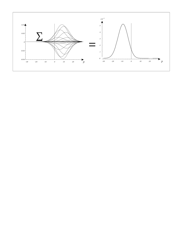
Figure 2.6: The net effect of superposing Gaussian packets shifted by positive integer values $\delta p=n$, and weighted by $e^{-|\lambda|^{2}}(-|\lambda|^{2})^{2}/n!$ with $\lambda=3$, is a packet shifted by the weak value $-|\lambda|^{2}=-9$. The scale of the resultant packet is an indication of how rarely the appropriate boundary conditions are realized. Nevertheless, if the conditions are in fact realized the measurement is almost certainly guaranteed to yield a negative reading.

At first sight, it appears that these significant effects pose a serious threat to causality, as it would then seem possible to do “fortune-telling”: in other words, to obtain information about the final state from a single event, before the choice of the post-selection basis is made. There are in fact two conditions ensuring that consistency with macroscopic causality is nevertheless maintained:

First of all, the fall-off condition of $\phi_{i}(x)$ resulting from the “weakness condition” ensures that the Fourier transform $\phi_{i}(p)$ is an analytic function in the complex $p$-plane at least on a strip containing the whole real $p$-axis. Thus, at the time that the datum is read, the analytic information necessary to reconstruct the shape of the packet is already available everywhere in $p$  [5].

Secondly, as mentioned earlier, any unusual features of the conditional distribution must be indistinguishable a priori, in other words, “covered” by the noise of the unconditional distribution $dP(p|\Psi_{i})$; hence, the prior probability of finding $p$ in the region of uncertainty around the unusual mean value, as an “error”, is already greater than the corresponding transition probability itself.

We should also note that in the reciprocal $x$-space, the unusual effects correspond to a phenomenon in Fourier analysis known as superoscillations. This phenomenon will be discussed in more detail in Sec. (6.1) in connection with our model.

2.7 The Weak Linear Model

Returning to the conditional distribution of the data in the case of a weak measurement, i.e., Eq. (2.40), what is interesting therefore is that the statistics can be approximately described in terms of an alternative linear model where the role of the “signal” $A$ is now played by the possible weak values of $A$. Let us give therefore a preliminary formalization of this model.

We define the Weak Liner Model, or WLM for short, as a statistical model in which the data from a von-Neumann linear measurement is viewed as arising from a displacement of the pointer variable proportional to the real part of the weak value. This weak value we take to be a definite property of every system belonging to a given pre- and post- selected ensemble described by complete boundary conditions. As we shall generally deal with cases where $\frac{\langle\psi_{\mu}|\hat{A}|\psi_{1}\rangle}{\langle\psi_{\mu}|\psi_{1}\rangle}\,$ has both real and imaginary parts, we adopt the convention that unless it is made clear from the context, the real part will be denoted generically by the symbol $\alpha_{\mu}$; we shall then refer to $\alpha$ simply as the “weak value”. The model thus reads

$$p_{f}=p_{i}+\alpha_{\mu}\,,$$ (2.43)

where

$$\alpha_{\mu}\equiv{\rm Re}\frac{\langle\psi_{\mu}|\hat{A}|\psi_{1}\rangle}{\langle\psi_{\mu}|\psi_{1}\rangle}\,.$$ (2.44)

As we have done so far, the index $\mu$ labels the transition (i.e., the pre-and post selected ensemble) which may or may not be known to have occurred. This uncertainty is then quantified by assigning probabilities $P_{\mu}$ to each of the possible transitions compatible with the information at hand. When dealing with averages over these transition probabilities, we shall find it useful to distinguish from the usual $\langle..\rangle$ averages within a given state. Transition averages will thus be denoted with a “bar”, so that for instance $\overline{\alpha}$ stands for

$$\overline{\alpha}\equiv\sum_{\mu}P_{\mu}\,\alpha_{\mu}\,.$$ (2.45)

Now, as it stands, the WLM is no more than a proposed way of interpreting the data, and in the same way that we saw for the SLM, one may expect that that its range of validity is quite limited. The claim is then that if the measurement satisfies appropriate conditions of weakness, where it may be supposed that the apparatus and the system behaved almost as separate entities, then the distribution of the data becomes approximately separable under the WLM.

As a preliminary check of consistency of this claim, suppose that such weakness conditions can be made to hold for all the transitions $|\psi_{1}\rangle\rightarrow|\psi_{\mu}\rangle$ defined by a particular post-selection. We should then be able to approximately interpret the unconditional statistics as a reflection of the “scatter” of weak values that follows from the dispersion in the possible final outcomes of the post selection. Since the weakness condition entails that the transition probabilities $P(\psi_{\mu}|\psi_{1})=|\langle\psi_{\mu}|\psi_{1}\rangle|^{2}$ are left practically unchanged, the statement translates to a sum rule in the form of a convolution

$$dP(p\,|\Psi_{f})\simeq\sum_{\psi_{\mu}}P(\psi_{\mu}|\psi_{1})\,dP(p-\alpha_{\mu}|\phi_{i})=\overline{dP(p-\alpha|\phi_{i})}\,.$$ (2.46)

Consider then unconditional expectation value of the data. According to the sum rule, this is given by

$$\overline{\langle p_{f}\rangle}=\langle p_{i}\rangle+\overline{\alpha}\,.$$ (2.47)

Note that we now interpret the unconditional expectation value of the data $\langle\Psi_{f}|\hat{p}|\Psi_{f}\rangle$ as the “bar-average” $\overline{\langle p_{f}\rangle}$ of the conditional averages $\langle\phi_{f}^{(\mu)}|\hat{p}_{f}|\phi_{f}^{(\mu)}\rangle$, whereas $\langle p_{i}\rangle=\langle\phi_{i}|\hat{p}|\phi_{i}\rangle$ remains the same as the “noise” distribution is here assumed to be independent of the transition. Computing now the bar average of the weak value,

$$\overline{\alpha} = \sum_{\mu}P(\psi_{\mu}|\psi_{1})\alpha_{\mu}\ ,$$ (2.48)

$$= {\rm Re}\sum_{\mu}|\langle\psi_{\mu}|\psi_{1}\rangle|^{2}\frac{\langle\psi_{\mu}|\hat{A}\,|\psi_{1}\rangle}{\langle\psi_{\mu}|\psi_{1}\rangle}$$

$$= {\rm Re}\langle\psi_{1}|\sum_{\mu}|\psi_{\mu}\rangle\langle\psi_{\mu}|\hat{A}|\psi_{1}\rangle\,$$

$$= \langle\psi_{1}|\hat{A}|\psi_{1}\rangle\,,$$

we indeed see that the mean displacement of the unconditional distribution is $\langle\psi_{1}|\hat{A}|\psi_{1}\rangle$, as we derived earlier in terms of the SLM. This illustrates how the standard expectation value of $\hat{A}$ may be interpreted either as the expectation value of the spectral distribution defined by $|\psi_{1}\rangle$, or just as well as the average of the weak values from the complete set of transitions defined by a particular post-selection.

Similar sum rules for higher moments cannot be interpreted exclusively from the “scatter” of weak values, but must take into account corrections to the transition probabilities and the widths of the unconditional distributions. Corrections to the sum rules will be examined more carefully in Chapter 5 in connection with the non-linear model.

2.8 Summary and Motivation for the Non Linear Model

Let us then summarize the general picture we have tried to present in this section. As we have seen, in regards to the functional form of the distribution of the data, there appears to be no qualitative distinction between ideal and non-ideal realizations of a von Neumann measurement of $\hat{A}$ when analyzed against initial conditions only (i.e., from a pre-selected ensemble); in either case the data can be interpreted under the SLM, i.e., as arising from the same spectral distribution, the only difference apparently being the amount of “noise” in the data. Furthermore, as the SLM is a $c$-number transcription of the Heisenberg evolution of the pointer variable operator, SLM consistency in the non-ideal case would naturally seem to imply the same dynamical picture of the ideal case. It is only when the data is analyzed against both initial and final boundary conditions that a clear distinction between ideal and non-ideal measurements emerges. The distinction is brought about by interference terms in the conditional distributions which do not show up in the unconditional distributions. These interference terms prevent the general statistical separability of the data under the SLM, except under an ideal apparatus preparation of sharp $p$ in which case a no-overlap condition is satisfied.

In contrast, there is the opposite weak regime of sharp $x$, where a “complementary ideal” is almost approached, namely that of physical separability or no entanglement between system and apparatus. In such case the interference terms are significant in the conditional distributions and the mechanical intuition behind the SLM picture is lost altogether. In exchange, however, an alternative picture emerges as the data becomes statistically separable under the WLM, in which the role of the signal is played by the weak value of $\hat{A}$. Even though this signal may take values well outside the spectrum of $\hat{A}$, it is nevertheless guaranteed by QM that the unusual systematic effects associated with weak values should remain hidden in the unconditional distributions as demanded by macroscopic causality

Chapter 3 Sampling Weak Values: An Illustrative Example

Our intention in this and the following chapter is to develop a preliminary intuition into the picture of “sampling weak values” that we wish to associate with the non-linear model. In this chapter, we introduce the concept of local weak values. The model itself will be developed formally in the Chapter 5.

3.1 Classical Angular Momentum as a Weak Value

Consider a free particle in two dimensional space prepared at a time $t_{1}$ in some initial sharp state in momentum, for simplicity an eigenstate $|k\rangle$, and post-selected at a time $t_{2}$ in the position eigenstate $|q\rangle$, where $\hat{q}$ and $\hat{k}$ are vector-valued and canonically conjugate to each other. For the intermediate measurement we take $\hat{A}$ to stand for the orbital angular momentum operator in two dimensions

$$\hat{L}=\hat{q}_{x}\hat{k}_{y}-\hat{q}_{y}\hat{k}_{x}\equiv\hat{q}\wedge\hat{k}\,.$$ (3.1)

Since the particle is assumed to be free, the free Hamiltonian commutes with $\hat{L}$ and the conditional statistics of the measurement will not depend on the intermediate time $t_{i}$; we may therefore take $t_{i}$ to be a time immediately before $t_{2}$; furthermore, as $|k\rangle$ is an eigenstate of the free evolution, it acquires a dynamical phase factor at $t=t_{2}$ which may be disregarded as it does not depend on the apparatus. It is then easy to see that for this pair of boundary conditions, the weak value of $\hat{L}$ is

$$\lambda=\frac{\langle q|\hat{q}\wedge\hat{k}|k\rangle}{\langle q|k\rangle}=q\wedge k\,.$$ (3.2)

Thus, between $t_{1}$ and $t_{2}$, the weak value of $L$ coincides with the conserved classical angular momentum defined by $q$ and $k$.

3.2 Sampling A Real Weak Value over a Narrow Window

Our starting point will be to examine in some detail a canonical example of how such weak values are realized when the dispersion in the conjugate variable $x$ is controlled, and as seen from the point of view of the $x$-representation. Recalling the definition of the relative state $|\phi_{f}^{(\mu)}\rangle$ corresponding to a given post-selection, i.e., Eq. (2.18), we see that in the $x$ representation the relative wave function $\phi_{f}^{(\mu)}(x)=\langle x|\phi_{f}^{(\mu)}\rangle$ is a product of two terms

$$\phi_{f}^{(\mu)}(x)=\langle\psi_{2}|e^{i\hat{A}x}|\psi_{1}\rangle\phi_{i}(x)\,.$$ (3.3)

For the boundary conditions in the present example, we then see that the wave function in the $p$-representation may be written as the Fourier integral

$$\phi_{f}(p)=\frac{1}{\sqrt{P(q|\Psi_{f})}}\int_{-\infty}^{\infty}\frac{dx}{\sqrt{2\pi}}\,e^{-ipx}\langle q|e^{i\hat{L}x}|k\rangle\phi_{i}(x)\,.$$ (3.4)

where we have dropped the transition index for simplicity.

The viewpoint that we wish to emphasize henceforth is that the integration variable $x$ parameterizes, as a back-reaction, a unitary transformation on the side of the system. The factor $\langle q|e^{i\hat{L}x}|k\rangle$ is then viewed as the transition amplitude from $|k\rangle$ to $|q\rangle$ mediated by an intermediate impulsive rotation of the system around the $z$ axis by an angle $x$. As we can see, the signs are such that the unitary operator $e^{i\hat{L}x}$ induces an active clockwise rotation by $x$ when acting on a ket; perhaps it is therefore more convenient to view the rotation as an active rotation of the final state $\langle q|e^{i\hat{L}x}=\left[\,e^{-i\hat{L}x}|q\rangle\,\right]^{\dagger}$, in which case the argument $q$ of the bra is taken to a new value $q(x)\equiv R(x)q\,$ where $R(x)$ is the ordinary counter-clockwise rotation matrix in two dimensional space. The transition amplitude is then

$$\langle q|e^{i\hat{L}x}|k\rangle=\langle q(x)|k\rangle=\frac{1}{2\pi}\,e^{iq(x)\cdot k}\,,$$ (3.5)

following trivially from the inner product between $\hat{q}$ and $\hat{k}$ eigenstates.

Similarly, from the viewpoint of the “reaction variable” $x$, the apparatus initial state $\phi_{i}(x)$ describes the prior experimental control on the back-reaction. Consider therefore the wave function $\phi_{i}(x)$ representing the tightest possible control on the back-reaction, namely, one from which the rotation angle $x$ is ensured not to deviate by more than $\epsilon$ from a mean angle $\tilde{x}$. This defines for us what we shall term a “window” test function, a square pulse of width $2\epsilon$ centered at $x=\tilde{x}$

$$\phi_{i}(x|\epsilon\,\tilde{x})=\left\{\begin{array}[]{cc}\frac{1}{\sqrt{2\epsilon}}&if\ |x-\tilde{x}|<\epsilon\\ 0&if\ |x-\tilde{x}|\geq\epsilon\end{array}\right.\,.$$ (3.6)

Its Fourier transform, which for simplicity we distinguish by the argument $p$ only, is the well-known “sinc” function

$$\phi_{i}(p|\epsilon\,\tilde{x})=\sqrt{\frac{\epsilon}{\pi}}\,\frac{\sin(p\,\epsilon)}{p\,\epsilon}e^{-ip\tilde{x}}\,.$$ (3.7)

In spite of the fact that the resultant probability distribution has an infinite variance, a natural width is nevertheless defined by $\pi/\epsilon$ as approximately $90\%$ of the probability mass is concentrated within the central lobe bounded by $p=\pm\pi/\epsilon$. If the dispersion in the back-reaction is therefore constrained to be less than a full rotation, i.e., $\epsilon<\pi$, it is then guaranteed that the “noise” will exceed the maximum required to clearly distinguish the integer-valued spectrum of $\hat{L}$, i.e., $\pi/\epsilon<1$.

It is under such small-angle conditions that the weak value of $\hat{L}$ becomes an appropriate description of the pointer variable response. As we can see, using (3.5) and (3.6), and taking care of the normalizing factor, the relative wave function for the window test function may be written as

$$\phi_{f}(p|\epsilon\,\tilde{x})=\frac{1}{\sqrt{4\pi\epsilon}}\int_{\tilde{x}-\epsilon}^{\tilde{x}+\epsilon}dx\,e^{-ip\,x+iS(x)}\,\,,$$ (3.8)

where the phase $S(x)$ is seen to be an oscillating function

$$S(x)=q(x)\cdot k=|q||k|\cos(x+\theta_{o})\,.$$ (3.9)

Here, $\theta_{o}$ is defined to be the angle from $k$ to $q$. From the integral representation (3.8), it is straightforward to derive an exact expression connecting the average shift, the expectation value of $\langle p\rangle_{f}=\langle\phi_{f}|\hat{p}|\phi_{f}\rangle$, with the phase gradient $S^{\prime}(x)$. For this one notes that since the support of the integrand is strictly bounded, $\phi_{f}(p|\epsilon\,\tilde{x})$ must be an entire function with all derivatives defined; we may then use the replacement $x\rightarrow i\frac{\partial}{\partial p}\,$ to pull the phase factor outside the integral and replace it for a differential operator

$$e^{iS\left(i\frac{\partial}{\partial p}\right)}\,.$$ (3.10)

The action of this operator on $p$ is then a self-adjoint operator with respect to the initial state $|\phi_{i}\rangle$:

$$e^{-iS\left(i\frac{\partial}{\partial p}\right)}\,p\,e^{iS\left(i\frac{\partial}{\partial p}\right)}=p+S^{\prime}\left(i\frac{\partial}{\partial p}\right)\,.$$ (3.11)

Thus, the expectation value of the data reads:

$$\langle p\rangle_{f}=\langle p\rangle_{i}+\langle S^{\prime}(x)\rangle$$ (3.12)

where $\langle p\rangle_{i}=\langle\phi_{i}|\hat{p}|\phi_{i}\rangle=0$ , and the average shift is the expectation value of the phase gradient over the sampled window:

$$\langle S^{\prime}(x)\rangle=\langle\phi_{i}|S^{\prime}(x)|\phi_{i}\rangle=\frac{1}{2\epsilon}\int_{\tilde{x}-\epsilon}^{\tilde{x}+\epsilon}dx\,S^{\prime}(x)\,.$$ (3.13)

Using the trigonometric form of $S(x)$ as given in Eq. (3.9), we may further express this average as

$$\langle S^{\prime}(x)\rangle=S^{\prime}(\tilde{x})\frac{\sin\epsilon}{\epsilon}\,,$$ (3.14)

which shows that a small angle condition on the sampling window $2\epsilon<1$, ensures that the average shift is essentially the phase gradient evaluated at the sampling point $\tilde{x}$. And finally, as one can then verify, this local phase gradient is in fact a weak value of $\hat{L}$,

$$S^{\prime}(x)=-i\frac{d}{dx}\log\,\langle q(x)|k\rangle=\frac{\langle q(x)|\hat{L}|k\rangle}{\langle q(x)|k\rangle}\,,$$ (3.15)

namely in this case the classical angular momentum $q(\tilde{x})\wedge k$ corresponding to a pre- and post selected ensemble where the final position eigenstate $|q\rangle$ is rotated by the angle $\tilde{x}$.

Thus we conclude that if the window and centered around some entirely arbitrary “sampling point” $\tilde{x}$, and is sufficiently narrow so that it satisfies a small angle condition, then the average conditional displacement of the pointer variable is essentially a weak value, what we shall call a local weak value $\lambda(x)=S^{\prime}(x)$, evaluated at the sampling point

$$\delta\langle p\rangle\simeq\lambda(\tilde{x})\equiv\frac{\langle q|e^{i\hat{L}\tilde{x}}\hat{L}|k\rangle}{\langle q|e^{i\hat{L}\tilde{x}}|k\rangle}\,.$$ (3.16)

The point therefore is that if one looks at $x$ as the angle parameter of the transformation induced by $\hat{L}$, then, as the transformation becomes a well-defined unitary transformation $\simeq e^{i\hat{L}\tilde{x}}$ by virtue of the small uncertainty $\Delta x$, then the local weak value evaluated at the mean angle determines the conditional response of the pointer variable. From this perspective, the “standard” weak value $\lambda=q\wedge k$ may hence be seen as the resulting shift in a special, canonical, weak measurement, namely one in which the sampling point approximately determines a null rotation of the system.

It is worth remarking that while the aforementioned result concerns the relation between the conditional expectation value of the pointer variable and the local weak value under small angle conditions, it does not say anything about the resultant shape of the pointer variable distribution obtained from $\phi_{f}(p|\epsilon\tilde{x})$. However, it is always possible to impose more restrictive conditions on the size $\epsilon$ in order to ensure that the shift occurs with minimal distortion of the overall shape of the initial packet $\phi_{i}(p|\epsilon\tilde{x})$, and hence of the resulting conditional probability distribution (Fig. 3.1).

As one sees, the Fourier integral (3.8) shows an analogy with the propagation of a an almost-monochromatic beam through a dispersive medium, where $x$ plays the role of the wave number and $S(x)$ the dispersion relation. The relative wave function $\phi_{f}(p|\epsilon\tilde{x})$ may thus be interpreted as the result of propagating the initial packet $\phi_{i}(p|\epsilon\tilde{x})$ through this medium after unit time, in which case the local weak value corresponds to the group velocity. If $\epsilon$ is therefore small enough that the non-linear behavior of the phase factor $S(x)$ around the sampling point may be neglected altogether, then the integral (3.8) can be performed in a “group velocity” approximation, in which case the relative wave function is up to phase factors the initial wave function rigidly translated by the local weak value $\lambda(\tilde{x})$

$$\phi_{f}(p|\epsilon\,\tilde{x}) \simeq \phi_{i}(p-\lambda(\tilde{x})|\epsilon\,\tilde{x})e^{i\left[S(\tilde{x})-\lambda(\tilde{x})\tilde{x}\right]}$$ (3.17)

$$= \sqrt{\frac{\epsilon}{\pi}}\,\frac{\sin\left[\,(p-\lambda(\tilde{x})\,)\epsilon\right]}{\left[\,(p-\lambda(\tilde{x})\,)\epsilon\right]}e^{i\,\left[S(\tilde{x})-p\tilde{x}\right]}\,.$$

Expanding the phase as

$$S(\tilde{x})+\lambda(\tilde{x})(x-\tilde{x})+\frac{1}{2}\lambda^{\prime}(\tilde{x})(x-\tilde{x})^{2}+...\,,$$ (3.18)

we see that the linearity condition is ensured if

$$\lambda^{\prime}(\tilde{x})\epsilon^{2}\ll 1.$$ (3.19)

While for small angular momenta ($|q||k|\ll 1$) linearity is essentially guaranteed by the small-angle condition on $\epsilon$, for $|q||k|\gg 1$ linearity demands a much tighter control of the dispersion in the rotation angle, namely $\epsilon\simeq O(1/\sqrt{|q||k|})$. This means that the shape of the initial packet is preserved when the effective width in the pointer variable $p$ is of order $\sqrt{|q||k|}$, which is considerably larger than the eigenvalue spacing. Note, however, that in the limit where $|q||k|\rightarrow\infty$, this large width nevertheless becomes insignificant relative to the overall shift in $p$, which should be of order $|q||k|$. This shows that for boundary conditions that are approximately classical, it is possible to guarantee a statistically significant effect on the pointer variable that is a rigid shift proportional to the classical angular momentum.

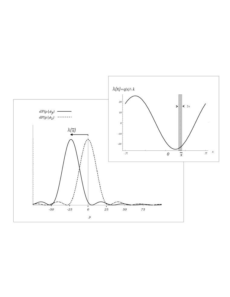
Figure 3.1: Sampling the local weak value $\lambda(\tilde{x})$ over a narrow window. In this example, $|q||k|=25$, $\theta_{o}=\pi/2$, $\tilde{x}=\pi/8$ and $\epsilon=\pi/32$. The system is therefore rotated by angle $\pi/8\pm\pi/32$, and the sampled weak value is approximately $\lambda(\tilde{x})\simeq-23$.

3.3 Superpositions of Weak Measurements

On the basis of this local picture, it is then possible to develop an alternative interpretation of the relative wave function $\phi_{f}(p)$ away from the weak regime, or in other words, when the dispersion in the back-reaction angle is considerable. For this we note that given an arbitrary initial apparatus state $|\phi_{i}\rangle$, the wave function in $x$ can always be “chopped” into non-overlapping windowed wave functions $\phi_{i}(x|n)$

$$\phi_{i}(x)=\sum_{n}\sqrt{P(n|\phi_{i})}\,\phi_{i}(x|n)$$ (3.20)

where

$$\phi_{i}(x|n) = \left\{\begin{array}[]{cc}\frac{\phi_{i}(x)}{\sqrt{P(n|\phi_{i})}}&if\ |x-\tilde{x}_{n}|<\epsilon_{n}\\ 0&if\ |x-\tilde{x}_{n}|\geq\epsilon_{n}\end{array}\right.\,,$$ (3.23)

$$P(n|\phi_{i}) = \int_{\tilde{x}_{n}-\epsilon_{n}}^{\tilde{x}_{n}+\epsilon_{n}}dx\,|\phi_{i}(x)|^{2}$$ (3.24)

and where say if $n$ and $n+1$ are contiguous cells, then $\tilde{x}_{n+1}-\tilde{x}_{n}=\epsilon_{n+1}-\epsilon_{n}$. If the “chopping” in Eq. (3.20) is sufficiently fine so that within each window either a small angle condition is satisfied, or, more restrictively, a local linear expansion of the phase is valid, then the relative wave function in the $p$ representation may be approximated as a coherent superposition of overlapping (but nevertheless orthogonal) wave functions, each of which gets shifted by the appropriate local weak value. In particular, if the “group velocity” approximation is valid within each window, then it is the overall shape of the Fourier transform $\phi_{i}(p|n)$ of each windowed function $\phi_{i}(x|n)$ which gets shifted, in which case the relative wave function expands as

$$\phi_{f}(p)\simeq\sum_{n}\sqrt{P(n|\phi_{i})}\,\phi_{i}(p-\lambda(\tilde{x}_{n})\,|n)\,e^{i[S(\tilde{x})-\lambda(\tilde{x})\tilde{x}]}.$$ (3.25)

Thus, one may think of a measurement given an arbitrary preparation of the apparatus as a coherent superposition of weak measurements, each sampling a weak value at a different sampling point $\tilde{x}_{n}$.

3.4 Illustration: Eigenvalue Quantization in a Strong Measurement

For the boundary conditions in question, the sampling picture suggests that when the initial pointer wave function $\phi_{i}(p)$ is sufficiently narrow that the eigenvalues of $\hat{L}$ become distinguishable, one may equivalently view the resultant conditional probability distribution as an interference effect arising from sampling the classical angular momentum over a large range of $x$.

We have tried to illustrate this interference effect in Figures (3.2) and (3.3) for the same boundary conditions of Fig. (3.1), $|q||k|=25$ and $\theta_{o}=\pi/2$, for which the local weak value is

$$\lambda(x)=-25\cos(x)\,.$$ (3.26)

The initial wave function is in this case taken to be a minimum uncertainty packet, in $x$

$$\phi_{i}(x)=(2\pi\sigma_{x}^{2})^{-1/4}\ e^{-\left(\frac{x}{2\sigma_{x}}\right)^{2}}$$ (3.27)

of spread $\sigma_{x}=\pi$. Its Fourier transform is then a Gaussian in $p$ with a spread $\sigma_{p}=1/2\pi\simeq 0.16$, which is much smaller than the eigenvalue separation. The sampling is performed at equal intervals of $x_{n}=n\pi/4$, so $\epsilon=\pi/8$ for each window. In the $p$ representation, each of the windowed functions $\phi_{i}(p|n)$ is then approximately a “sinc” function centered at $p=0$, and modulated by a phase factor $\simeq e^{-ipx_{n}}$, as in Eq. (3.7). Each of these gets shifted approximately by the local weak value $\lambda(\tilde{x}_{n})=-|q||k|\cos(\tilde{x}_{n})$. To illustrate how $\phi_{f}(p)$ is built up from the interference of the shifted windowed functions $\phi_{f}(p|n)$, Fig. (3.2) shows the real part of the latter, scaled by the appropraite weights $\sqrt{P(n|\phi_{i})}$. The net sum of the imaginary parts cancels out by symmetry. The cosine curve of $\lambda(x)$, also shown in Fig. (3.1), is clearly appreciable from the array of these shifted functions. Note that the amplitude of this curve determines the region where the resultant probability distribution, shown in Fig. (3.3), is appreciable.

The emergence of a quantized structure in this distribution may then be understood from the periodicity of the weak value as follows: to a given window with $\tilde{x}_{n}\in[-\pi,\pi)$, there correspond an infinite number of other windows at different winding numbers, i.e., $\tilde{x}_{n}\pm 2\pi,\ \tilde{x}_{n}\pm 4\pi,\ ...$, where the same weak value is sampled. Each of these “secondary” samples yields approximately the same partial wave function, except for an additional relative phase factor $e^{\mp ip2\pi},\ e^{\mp ip4\pi},\ ...$, weighted by a relatively slow-decaying weight factor $\sqrt{P(n|\phi_{i})}$. The phases therefore interfere constructively when $p$ is an integer and destructively when $p$ is a half integer. Very roughly, then, one may understand the resultant interference pattern in $\phi_{f}(p)$ as the product of two terms: First, a rapidly varying factor

$$\sum_{n=-\infty}^{\infty}\sqrt{P(n|\phi_{i})}e^{ip2n\pi}\sim\sum_{m=-\infty}^{\infty}\Delta(p-m)$$ (3.28)

where $\Delta(p)$ is a sharply peaked function at $p=0$. This accounts for the global periodic behavior of the local weak value. The second factor yields an envelope to the modulation factor which accounts for the average contribution of the samples within a given period, for instance the samples $\tilde{x}_{n}$ lying between $-\pi$ and $\pi$. To a first approximation, the envelope may be obtained by replacing the Gaussian shape of $\phi_{i}(x)$ for a flat distribution within the interval, in which case the resultant wave function is proportional to that of a window test function centered at $\tilde{x}=0$ and covering one complete revolution, i.e., $\epsilon=\pi$:

$$\phi_{f}(p|\tilde{x}=0,\epsilon=\pi)=\frac{1}{2\pi}\int_{-\pi}^{\pi}dx\,e^{-ipx-i|q||k|\sin(x)}\,.$$ (3.29)

This rough decomposition becomes increasingly accurate in the limit $\sigma_{x}\rightarrow\infty$, where the product $\phi_{i}(x)e^{iS(x)}$ becomes invariant under translations in $x$ modulo $2\pi$; the two factors (3.28) and (3.29) correspond then to a decomposition in terms of Bloch states, with the $\Delta(p)$ in (3.28) replaced by a true $\delta(p)$.

A consequence of this decomposition is then that up to a normalization, the second factor must yield for integer values $p=m$ the transition amplitude $\langle q|\hat{\Pi}(m)|k\rangle$ for an intermediate projection onto an eigenvalue $m$ of $\hat{L}$. For such values, the integral is easily obtained in closed form in terms of Bessel functions:

$$\phi_{f}(p=m|\tilde{x}=0,\epsilon=\pi)=(-1)^{m}J_{m}(|q||k|)\,.$$ (3.30)

A continuous envelope for the probability distribution, indicated in Fig. (3.3) by the dotted line, is then $J_{|p|}^{2}(|q||k|)$ times an appropriate normalization constant.

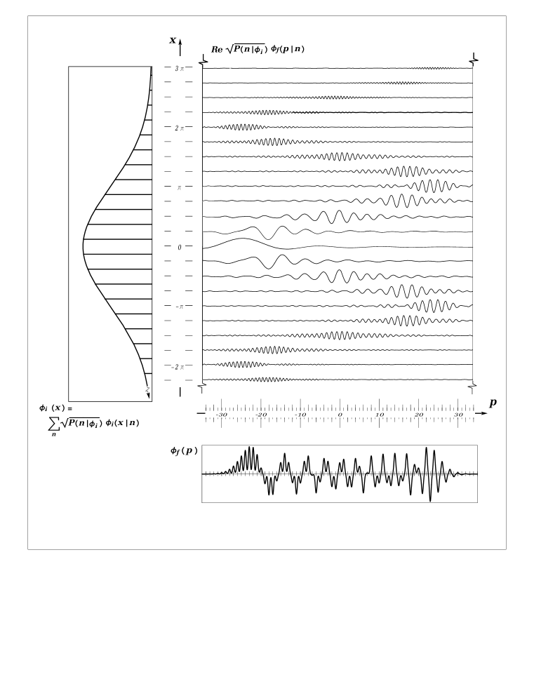
Figure 3.2: A relative wave function for a strong measurement built up as a superposition of weak measurements (see text).

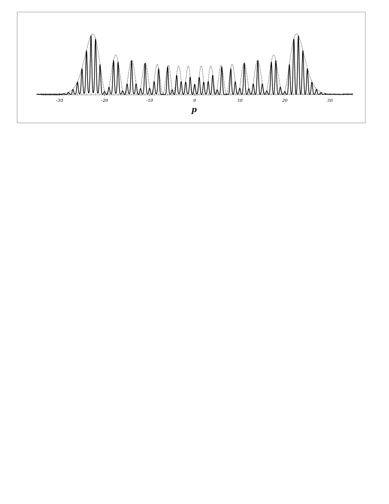
Figure 3.3: The resultant probability distribution function $\phi_{f}^{2}(p)$, and its envelope $\propto J_{|p|}^{2}(|q||k|)$.

3.5 Error Laws

Since the measurement is in this case clearly a strong measurement, the trace of weak values, when seen from the sampling picture, is practically washed out by the interference of the different samples. It is nevertheless instructive to note how two statistics of the resultant probability distribution can nevertheless still be connected to the picture of sampling weak values:

First of all, let us note the trace that remains from the fact that the dominant sample is the one centered at $\tilde{x}=0$ where the weak value is $-|q||k|$. This can be seen clearly from the asymmetry in the wave function $\phi_{f}(p)$ in Fig. (3.2), an asymmetry that is barely noticeable once the amplitudes are squared as seen in Fig (3.3). Nevertheless, the asymmetry leads to a slight bias of the distribution towards the predominantly sampled weak value, a bias that is absent altogether in an ideal strong measurement. The bias or the mean displacement $\langle p\rangle_{f}=\langle\phi_{f}|\hat{p}|\phi_{f}\rangle$, is easily calculated as was done earlier for the case of a narrow window. We note that a Gaussian wave function has all moments defined for both $x$ and $p$ and is analytic in either domains. Thus, the effect of multiplying $\phi_{i}(x)$ by a phase factor $e^{iS(x)}$ may again also be described in the Heisenberg picture as a shift of the pointer variable operator

$$\hat{p}_{f}=\hat{p}_{i}+S^{\prime}(\hat{x})=\hat{p}_{i}+\lambda(\hat{x})\,.$$ (3.31)

Thus, for a Gaussian initial state $|\phi_{i}\rangle$ centered initially at zero in $p$, the average conditional shift is

$$\langle p_{f}\rangle=\langle\lambda(\hat{x})\rangle$$ (3.32)

where $\langle\lambda(\hat{x})\rangle$ is the expectation value of the local weak value over the probability distribution in $x$ , $dP(x|\phi_{i})=dx|\phi_{i}(x)|^{2}$:

$$\langle\lambda(\hat{x})\rangle=\int_{x}dP(x|\phi_{i})\lambda(x)\,.$$ (3.33)

It is truly then the average sampled weak value in the limit where the samples become infinitesimally narrow. For a normal distribution in $x$, centered at $x=0$ and with $\lambda(x)=-|q||k|\sin(x+\theta_{o})$, the mean weak value is easily obtained:

$$\langle\lambda(x)\rangle=\lambda(0)\,e^{-\sigma_{x}^{2}/2}\,.$$ (3.34)

The mean conditional displacement is hence the weak value evaluated at the peak of the distribution and scaled by an exponential suppression factor $e^{-\sigma_{x}^{2}/2}$.

A more notorious trace of the sampling picture is, as mentioned earlier, the connection that exists between the amplitude of the weak value curve and the width of the resultant probability distribution. This connection can now be expressed in terms of an intuitive “error” law connecting the initial and final variances $\Delta p_{i}^{2}=\langle\phi_{i}|\hat{p}^{2}|\phi_{i}\rangle$, and $\Delta p^{2}_{f}=\langle\phi_{f}|\hat{p}^{2}|\phi_{f}\rangle-\langle p\rangle_{f}^{2}$, which follows from Eq. (3.31). Taking the square of this equation we have

$$\hat{p}^{2}_{f}=\hat{p}_{i}^{2}+\{\hat{p}_{i},\lambda(\hat{x})\}+\lambda(\hat{x})^{2}\,.$$ (3.35)

It is easily shown that for the Gaussian packet, the expectation value of the anti-commutator of $\hat{p}$ and $\lambda(\hat{x})$ vanishes. Thus, we have

$$\Delta p_{f}^{2}=\Delta p_{i}^{2}+\Delta\lambda^{2}$$ (3.36)

where $\Delta\lambda^{2}$ is the variance $\langle\lambda(x)^{2}\rangle-\langle\lambda(x)\rangle^{2}$ of the local weak value over the probability distribution $dP(x|\phi_{i})$:

$$\Delta\lambda^{2}=\int_{x}dP(x|\phi_{i})\left(\lambda(x)-\langle\lambda(x)\rangle\right)^{2}\,.$$ (3.37)

Again this corresponds to the variance of the sampled weak values in the limit of infinitely narrow samples. In our case this variance is given by

$$\Delta\lambda^{2}=\frac{|q|^{2}|k|^{2}}{2}\left(1-e^{-\sigma_{x}^{2}}\right)^{2}\simeq\frac{|q|^{2}|k|^{2}}{2}\,,$$ (3.38)

which is essentially the r.m.s. value of the local weak value $\lambda(x)$ on its curve.

Finally, to see that these quantities do in fact coincide in the limit of strong measurements with similar quantities obtained from the conditional spectral distribution, we recall that this spectral distribution is given by

$$P(m|qk)\propto J_{m}^{2}(|q||k|)\,.$$ (3.39)

In fact, we note that the proportionality constant is unity since the Bessel functions satisfy

$$\sum_{m=-\infty}^{\infty}J_{m}^{2}(z)=1$$ (3.40)

for all $z$. The conditional average of $m$ is then

$$\langle m\rangle=\sum_{m=-\infty}^{\infty}J_{m}^{2}(z)m$$ (3.41)

which vanishes by symmetry. This coincides with Eq. (3.34) in the limit $\sigma_{x}\rightarrow\infty$. Similarly, we note the identity

$$\langle m^{2}\rangle=\sum_{m=-\infty}^{\infty}J_{m}^{2}(z)m^{2}=\frac{z^{2}}{2}\,.$$ (3.42)

Letting $z=|q||k|$, we see that again this coincides with Eq. (3.38) in the same limit.

3.6 Summary: Local Weak Values

In chapter 2 we saw how relative to a given post-selection, the unconditional statistics of the pointer variable break up as

$$dP(p|\Psi_{f})=\sum_{\mu}P(\psi_{\mu}|\Psi_{f})dP(p|\phi_{f}^{(\mu)})$$ (3.43)

where $dP(p|\phi_{f}^{(\mu)})$ is the conditional probability distribution of the pointer variable obtained from the state of the apparatus relative to a final condition $|\psi_{\mu}\rangle$:

$$|\phi_{f}^{(\mu)}\rangle=\frac{1}{\sqrt{P(\psi_{\mu}|\Psi_{f})}}\ \ \langle\psi_{\mu}|e^{i\hat{A}\hat{x}}|\psi_{1}\rangle\,|\phi_{i}\rangle\,\,.$$ (3.44)

It was furthermore argued that when the initial apparatus state satisfied appropriate weakness conditions, this conditional distribution could be interpreted approximately in terms of a weak linear model (WLM) as

$$dP(p|\phi_{f}^{(\mu)})\simeq dP(p-\alpha_{\mu}|\phi_{i})\,,$$ (3.45)

where $alpha_{\mu}={\rm Re}\frac{\langle\psi_{\mu}|\hat{A}|\psi_{1}\rangle}{\langle\psi_{\mu}||\psi_{1}\rangle}$. The picture that we then wished to associate with this model was that when the conditions of the measurement are such that the measured system and the apparatus behave almost as independent entities, the system imparts a well-defined “kick” to the apparatus proportional to $\alpha_{\mu}$. Our purpose then was to see how this picture could be extended to more general apparatus conditions that do not satisfy the appropriate requirements of weakness.

This is the picture of sampling weak values for which we gave a preliminary illustration in this chapter. What we have illustrated here is that in the case where the transition amplitude in Eq. (3.44) is a pure phase factor, i.e,

$$\langle\psi_{\mu}|e^{i\hat{A}\hat{x}}|\psi_{1}\rangle=(const)e^{iS(x)}$$ (3.46)

where $S(x)$ is a real function of $x$, it is possible to develop a simple picture of the relative state as a coherent superposition of weak measurements. The idea is then to think of the initial state of the apparatus as a superposition of non-overlapping “sample states”, each of which has a wave function in the $x$ representation of bounded support within $\pm\epsilon_{n}$ around a given value $\tilde{x}_{n}$. Each sample may then be considered as implementing a weak measurement if the variation of the phase gradient $S^{\prime}(x)$ is small within the interval $\tilde{x}_{n}\pm\epsilon_{n}$, in which case the mean displacement of the pointer variable is essentially a local weak value of the measured observable $\hat{A}$, evaluated in a configuration where the initial and final state vectors are rotated relative to each other in Hilbert space by an intermediate unitary transformation $e^{i\hat{A}\tilde{x}_{n}}$:

$$\alpha_{\mu}(x)=S^{\prime}(\tilde{x}_{n})={\rm Re}\frac{\langle\psi_{\mu}|\hat{A}e^{i\hat{A}\tilde{x}_{n}}|\psi_{1}\rangle}{\langle\psi_{\mu}|e^{i\hat{A}\tilde{x}_{n}}|\psi_{1}\rangle}\,.$$ (3.47)

Finally, we saw how despite the fact that in the general, non-weak, case the shape of the pointer variable wave function is significantly altered because of interference between the different samples, it is nevertheless still possible to connect the picture of sampling weak values to two statistics of the conditional pointer variable distribution $dP(p|\phi_{f}^{(\mu)})$, namely the mean and the variance of $p$, according to:

$$\langle p\rangle_{f} = \langle p\rangle_{i}+\langle\alpha_{\mu}(x)\rangle$$

$$\Delta p_{f}^{2} = \Delta p_{i}^{2}+\Delta\alpha_{\mu}^{2}$$ (3.48)

where $\langle p\rangle_{i}$ and $\Delta p_{i}^{2}$ are the initial mean and variance of the pointer variable and $\langle A_{w}(x)\rangle$ and $\Delta A_{w}(x))^{2}$ are the mean and variance of the local weak value evaluated over the probability distribution for $x$ defined by the initial state of the apparatus, i.e. $dP(x|\phi_{i})=dx\,|\phi_{i}(x)|^{2}$. The latter correspond then to the mean and variance of sampled local weak values in the limit when the samples become infinitesimally narrow in $x$.

The problem that concerns us now is how to interpret the picture of sampling weak values in the more general situation in which the amplitude function $\langle\psi_{\mu}|e^{i\hat{A}x}|\psi_{1}\rangle$ in (3.44) is not necessarily a pure phase factor. From the point of view of the weak measurement regime, this more general situation would entail an imaginary component of the local weak value, and the associated effects that were briefly mentioned in the last chapter.

The contention here is however that a more convenient and intuitive description is provided by trading in this imaginary component for another real function, which we shall simply call the “likelihood factor” $L_{\mu}(x)$, defined as

$$L_{\mu}(x)=\frac{\|\langle\psi_{\mu}|e^{i\hat{A}x}|\psi_{1}\rangle\|^{2}}{P(\psi_{\mu}|\Psi_{f})}\,.$$ (3.49)

The intuition stems from a correspondence, both formal and in particular cases quantitative, that can be established between the sampling picture based on $\alpha_{\mu}(\hat{x})$ and $L_{\mu}(\hat{x})$ and a classical probabilistic description of the measurement interaction with mixed boundary conditions on the system.

Chapter 4 Bayes’ Theorem and Retrodiction in Classical Measurement

The second insight into the model comes from drawing parallels with the classical description of the measurement. According to classical mechanics, it should in principle be possible to measure any quantity, with perfect precision, and without back-reaction on the system. This ideal situation demands however an ideal control of the initial conditions of the apparatus which may not be available. As it then turns out, the problem of retrodiction in the classical description is not entirely trivial once this control is lost. The problem has to do with the fact that as we move forward in time, the probabilities we assign to the classical state of a system, i.e., the point in phase space, may change in either of two ways: because of the mechanical evolution, or else because of acquisition of new information. When the system is controlled for both initial and final conditions, both “effects” are confounded in the probabilities and some care is needed to disentangle them. Fortunately, the classical description provides sufficiently clear formal criteria to distinguish what is “mechanics” and what is “information”. Our aim will then be to establish a formal correspondence between these criteria and elements in the quantum description.

4.1 Prior and Posterior Probabilities

According to the Bayesian view of probability [20, 21, 22], a probability statement about a possible situation $X$ is always viewed relative to a particular set of stated conditions $Y$. Hence the symbol

$$P(X|Y)$$ (4.1)

to denote the probability of $X$ when $Y$ is known. A typical problem of inference occurs when one starts with knowledge only of $Y$, but later finds out additional information, for instance, that a certain other condition $Z$ is indeed satisfied. If $Z$ is a relevant condition, then one intuitively expects the probabilities to change. The problem is then to find how the a priori probabilities are modified to a posteriori probabilities in light of this additional condition. The solution to this problem is given by Bayes’ theorem.

To see how this comes about, we recall the product rule of probability, which states that

$$P(XZ|Y)=P(X|YZ)P(Z|Y)\,.$$ (4.2)

where $XZ$ stands for $X$ “and” $Z$. The product rule can however be applied in the reverse order, in which case

$$P(XZ|Y)=P(Z|XY)P(Z|Y)\,.$$ (4.3)

Equating (4.2) and (4.3), we find that

$$P(X|YZ)=P(X|Y)\frac{P(Z|XY)}{P(Z|Y)}\,.$$ (4.4)

The last line is Bayes’ theorem. It states that the posterior probability of $X$ given $Y$ and $Z$, is the prior probability of $X$ given $Y$, multiplied by a factor

$$L_{Z}(X)=\frac{P(Z|XY)}{P(Z|Y)}\,,$$ (4.5)

commonly known as the Likelihood factor. The effect of this factor is to increase (decrease) the prior probability for those values of $X$ for which $Z$ is more (less) likely to occur given $Y$ and $X$, as one may expect intuitively.

We finally note to facts about the passage from prior to posterior distributions:

First, from the product and sum rules, it is easy to see that the probability $P(Z|Y)$ in the denominator of the Likelihood factor is

$$P(Z|Y)=\sum_{X}P(ZX|Y)=\sum_{X}P(Z|XY)P(X|Y)\,.$$ (4.6)

This tells us that $P(Z|Y)$ can be determined from the normalization condition on the posterior probability as expected.

Second, while the posterior probability can be determined from knowledge of the conditional probability $P(Z|XY)$ and the prior probability $P(X|Y)$ for all values of $X$, it is generally not possible to determine the prior probability from knowledge of the posterior probability and $P(Z|XY)$ alone. This can clearly be seen if we consider a situation in which $P(Z|XY)$ is zero for a given range of $X$. In this case, any number of prior probability distributions are compatible with the same posterior probability. This tells us then that the transformation from prior to posterior probability with a fixed likelihood factor $L(X)\propto P(Z|XY)$ is generally an irreversible mapping in the space of probability distributions.

4.2 Prior Phase-Space Distribution

We shall now consider a simple classical caricature of the von Neumann scheme as we developed it in Chapter 2. Here we envision the apparatus as being described by classical canonical variables $x,p$, and the system described by a set of generalized canonical coordinates $\eta$. The measurement interaction is then described by a classical von-Neumann Hamiltonian

$$H_{M}=-\delta(t-t_{i})xA(\eta)\,.$$ (4.7)

Now, denoting the states immediately before and after the measurement by the suffixes $i$ and $f$, we can see that the Hamiltonian has two constants of the motion, $x$ and $A(\eta)$, and thus:

$$x_{f}=x_{i}\ \ \ A(\eta_{i})=A(\eta_{f})\,.$$ (4.8)

From this we know that the pointer variable indeed receives a kick proportional to the value of $A$ at the time of the measurement

$$p_{f}=p_{i}+A(\eta_{i})\,,$$ (4.9)

On the other hand, the Hamiltonian also drives as a back-reaction other variables of the system which are not invariant under the phase-space flow induced by $A(\eta)$. Thus, the most we can say is that the final state of the system $\eta_{f}$ is connected to the initial state through some map

$$\eta_{f}=\mu(\eta_{i},x)$$ (4.10)

solving the dynamical equation

$$\frac{\partial\mu(\eta,x)}{\partial x}=\{A(\eta)\,,\mu(\eta,x)\,\}_{PB}\,,\ \ \ \ \ \mu(\eta,x=0)=\eta\,,$$ (4.11)

where $\{A(\eta)\,,\mu(\eta,x)\,\}_{PB}$ is the Poisson bracket.

So now suppose we start with some prior information $Y=Y_{s}Y_{a}$ about the the initial state of the system and the apparatus, which is entails a factorable probability distribution

$$dP(x,p_{i},\eta_{i}|Y)=dP(x,p_{i}|Y_{a})dP(\eta_{i}|Y_{s})\,,$$ (4.12)

where we drop the label for $x$ as it is a constant of the motion. To obtain the prior distribution for the final point in phase space, we then use the solutions to the equations of motion,i.e. Eqs. (4.9),(4.10)

$$dP(x,p_{f},\eta_{f}|Y)=\int_{x,p_{i},\eta_{i}}\delta(p_{f}-p_{i}-A(\eta_{i}))\delta(\eta_{f}-\mu(\eta_{i},x))dP(x,p_{i}|Y_{a})dP(\eta_{i}|Y_{s})\,.$$ (4.13)

This transformation may also be viewed in the more familiar passive sense, i.e., as a map in the space of phase-space distributions

$$dP(x,p,\eta_{i}|Y;i)\rightarrow dP(x,p,\eta_{f}|Y;f)\,,$$ (4.14)

in which case we view the point in phase-space as held fixed and the distribution function evolving from $dP(x,p,\eta|Y;i)=dP(x,p|Y_{a};i)dP(\eta|Y_{s};i)$ to the new distribution $dP(x,p,\eta|Y;f)$ according to Liouville flow. Denoting the generator of phase flow associated with a given function $f$ as

$$\pounds_{f}\equiv\{f\,,\ \ \}_{PB}\,,$$ (4.15)

and for simplicity defining the generator of the phase flow induced by the measurement as

$$\pounds_{S}\equiv A(\eta)\pounds_{x}+x\pounds_{A}\,,$$ (4.16)

the final prior distribution is then

$$dP(x,p,\eta|Y;f) = e^{-\pounds_{S}}dP(x,p,\eta|Y;i)$$ (4.17)

$$= dP(x,p-A(\eta)|Y_{a};i)e^{-x\pounds_{A}}dP(\eta|Y_{s};i)\,.$$

It is clear that this transformation is reversible as it may may be undone by a second application of the inverse Liouville flow operator $e^{\pounds_{S}}$.

4.3 Posterior Distribution

Consider however what happens when we acquire, by some other means, new information $Z_{s}$ about the state of the system after this measurement interaction. Since the probability of $Z_{s}$ now depends on the back-reaction on the system, we must then re-assess all our prior information, both about the initial and final points in phase-space. To do this let us use Bayes’ theorem as described above to obtain the posterior distribution for the initial state:

$$dP(x,p_{i},\eta_{i}|YZ_{s}) = dP(x,p_{i},\eta_{i}|Y)\,\frac{P(Z_{s}|x,p_{i},\eta_{i}Y)}{P(Z_{s}|Y)}$$ (4.18)

$$= dP(x,p_{i}|Y_{a})dP(\eta_{i}|Y_{s})\,\frac{P(Z_{s}|x,p_{i},\eta_{i}Y)}{P(Z_{s}|Y)}.$$

Now, as the condition $Z_{s}$ on the system was obtained independently of the apparatus and after the measurement interaction, it will depend only on the final phase-space point $\eta_{f}$ of the system; hence,

$$P(Z_{s}|x,p_{i},\eta_{i}Y)=\int_{\eta_{f}}dP(\eta_{f}|x,p_{i},\eta_{i}Y)P(Z_{s}|\eta_{f})\,.$$ (4.19)

Moreover, as this final point is connected via the mapping $\mu(\eta_{i},x)$ in Eq. (4.10) only to $\eta_{i}$ and $x$, we have

$$dP(\eta_{f}|x,p_{i},\eta_{i}Y)=d\eta_{f}\,\delta(\eta_{f}-\mu(\eta_{i},x))\,.$$ (4.20)

This allows us to eliminate the conditions that are irrelevant for $Z_{s}$ given $x$ and $\eta_{i}$ in the likelihood ratio

$$\frac{P(Z_{s}|x,p_{i},\eta_{i}Y)}{P(Z_{s}|Y)}=\frac{P(Z_{s}|x\eta_{i})}{{P(Z_{s}|Y)}}\,.$$ (4.21)

Thus the posterior distribution for the initial state reads

$$dP(x,p_{i},\eta_{i}|YZ_{s})=dP(x,p_{i}|Y_{a})dP(\eta_{i}|Y_{s})\,L_{Z_{s}}(x\eta_{i})\,,$$ (4.22)

where the likelihood factor is

$$L_{Z_{s}}(x\eta_{i})=\frac{P(Z_{s}|x\eta_{i})}{{P(Z_{s}|Y)}}\propto\int d\eta_{f}\delta(\eta_{f}-\mu(\eta_{i},x))P(Z_{s}|\eta_{f})\,.$$ (4.23)

What we see therefore is that by including final conditions on the system, conditions which are dynamically connected to the initial conditions $\eta_{i}$ and the reaction variable $x$, the degrees of freedom of the system and the apparatus are correlated in a non-trivial fashion in the posterior initial distribution.

The correlation is then propagated forward in time to the final posterior distribution. As in the case of the prior distribution, the map

$$dP(x,p,\eta|YZ_{s};i)\rightarrow dP(x,p,\eta|YZ_{s};f)$$ (4.24)

from posterior initial distribution to posterior final distribution is a reversible map expressible in terms of the flow operator $e^{\pounds_{S}}$. What is important to note, however, is that the map from the prior initial distribution to the posterior final distribution,

$$dP(x,p,\eta|Y_{s};i)\rightarrow dP(x,p,\eta|YZ_{s};f)\,$$ (4.25)

is not a reversible map. The map is given by

$$dP(x,p,\eta|YZ_{s};f) = e^{{\pounds}_{S}}dP(x,p,\eta|Y;i)L(x\eta)$$ (4.26)

$$= dP(x,p-A(\eta)|Y_{a};i)e^{x\pounds_{A}}dP(\eta|Y_{s};i)L(x\eta)$$

and hence involves two types of transformations

1. an irreversible part corresponding to probability re-assessment, which is given by multiplication by the likelihood factor.

2. a reversible part describing the phase flow, which is given by the action of the operator $e^{{\pounds}_{S}}$.

4.4 Sampling

We shall find it convenient to re-express (4.18 ) in a manner in which the the logical dependence between the variables becomes more explicit. For this we take the likelihood ratio and re-write it as:

$$\frac{P(Z_{s}|x\eta_{i})}{P(Z_{s}|Y)}=\frac{P(Z_{s}|x\eta_{i})}{P(Z_{s}|xY_{s})}\frac{P(Z_{s}|xY_{s})}{P(Z_{s}|Y)}\,.$$ (4.27)

As one can then see from Bayes’ Theorem, the posterior probability of $\eta$, given x, is given by

$$dP(\eta_{i}|Y_{s}x)=dP(\eta_{i}|Y_{s})\frac{P(Z_{s}|x\eta_{i})}{P(Z_{s}|xY_{s})}$$ (4.28)

assuming, as we have done, that $x$ is irrelevant to $\eta_{i}$ a-priori. Similarly, the posterior apparatus phase space distribution is

$$dP(x,p_{i}|YZ_{s})=\,dP(x,p_{i}|Y_{a})\frac{P(Z_{s}|xY_{s})}{P(Z_{s}|Y)}$$ (4.29)

This allows us to write the posterior initial distribution for the system and apparatus, now in the passive sense, as

$$dP(x,p\eta|YZ_{s};i)=dP(x,p|Y_{a};i)dP(\eta|xY_{s}Z_{s};i)L_{Z_{s}}(x)\,,$$ (4.30)

where the likelihood factor is now only a function of the reaction variable $x$; passively, the likelihood factor is given by

$$L_{Z_{s}}(x)\propto\int_{\eta}\left[e^{-x\pounds_{A}}\,dP(\eta|Y_{s};i)\right]P(Z_{s}|\eta;f)\,\,,$$ (4.31)

where $P(Z_{s}|\eta;f)$ is the probability $P(Z_{s}|\eta)$ at the time referred to by $Z_{s}$, and propagated using the system’s free evolution back to the time immediately after the measurement. Finally, to obtain the final distribution from Eq. (4.30) we apply the phase flow $\pounds_{S}$ as before.

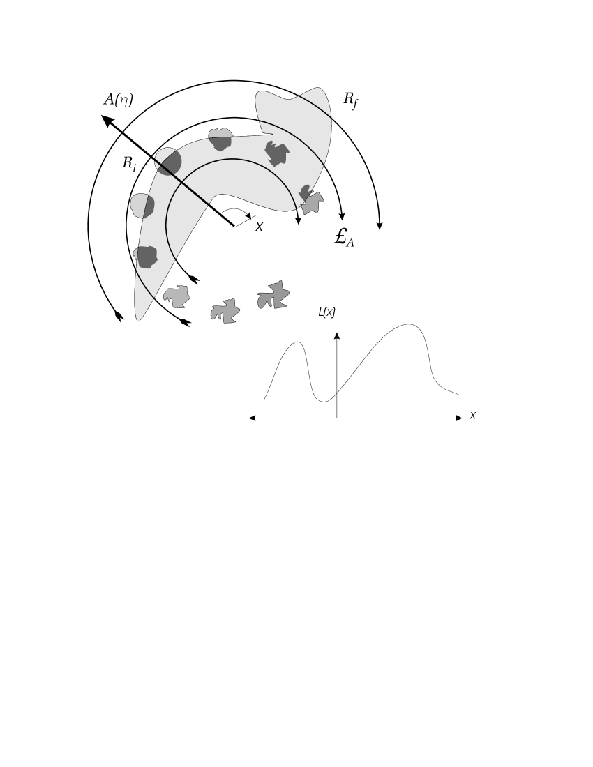
Figure 4.1: Phase space illustration of the posterior distribution (4.30. The initial and final conditions correspond to the lightly shaded regions $R_{i}$ and $R_{f}$. The initial region is then deformed by the transverse flow generated by $A$ and parameterized by the reaction variable $x$. A posterior distribution for $\eta$ given a value of $x$ corresponds to one the darkly shaded overlap regions. The likelihood factor for a given $x$ is proportional to the volume of the corresponding region.

To get some intuition for Eq. (4.30), think of the initial and final conditions on the system as two distinct regions $R_{i}$ and $R_{f}$ in its phase space as illustrated in Fig. (4.1). Given a specific value of $x$, the initial region is then deformed by the phase flow generated by $A(\eta)$ (i.e., the mapping $\mu(\eta_{i},x)$) to some other region $R_{i}(x)=e^{x\pounds_{A}}R_{i}$. The conjunction of the initial and final conditions given $x$ corresponds then to the region $R_{if}(x)=R_{i}(x)\bigcap R_{f}$ where the two regions overlap. This region determines the posterior final distribution $dP(\eta|xY_{s}Z_{s};f)$. The posterior initial distribution is then obtained by “undoing” the flow on the intersecting regions. Since the parameter $x$ is uncertain, the specific intersecting region that is sampled according to $x$ becomes uncertain as well. The probability that a given region $R_{if}(x)$ is sampled is then given by the posterior probability in $x$, which is the prior probability times the likelihood factor $L_{Z_{s}}(x)$. Within this picture, the likelihood factor is easily understood: it is proportional to the relative volume of the sampled intersecting region $R_{if}(x)$.

4.5 Conditional Distribution of The Data

We now wish to see what the likelihood factor entails classically in terms of the analysis of the data. Concentrating on the relevant variables, we introduce the posterior distribution of $A$ given $x$,

$$dP(A|xY_{s}Z_{s})=dA\int_{\eta}dP(\eta|xY_{s}Z_{s};i)\,\delta(A-A(\eta))\,,$$ (4.32)

i.e., the probability of $A$ within one of the intersecting regions $R_{if}(x)$. In terms of this distribution, we then have for the initial posterior distributions of the pointer variable

$$dP(p|YZ_{s};i) = \int_{x}dP(x,p_{i}|Y_{a})L_{Z_{s}}(x)\,$$

$$dP(p|YZ_{s};f) = \int_{xA}dP(x,p-A|Y_{a};i)dP(A|xY_{s}Z_{s};i)L_{Z_{s}}(x)\,$$ (4.33)

These we may now compare to the corresponding prior distributions, that is, without the classical post-selection on the system:

$$dP(p|Y;i) = \int_{x}dP(x,p|Y_{a};i)\,$$

$$dP(p|Y;f) = \int_{A}dP(A|Y_{s};i)dP(p-A|Y_{a};i)\,.$$ (4.34)

What we see here is an interesting situation that is somewhat evocative of the discussion in Chapter 2:

We observe that in the prior case, the final distribution of the data takes the simple separable form of a convolution with the prior distribution for the “signal” $A$. On the other hand, the same form is not attained in the posterior case; instead, separability is attained only in the mixed form, i.e., as in Eq. (2.15), with the role of the “mixing parameter” $\chi$ in that equation now being played by the reaction variable $x$ of the apparatus. In other words, what Eq. (4.33) shows is that, in contrast to the case of a pre-selected sample, prior information about the reaction variable is relevant in the proper analysis of the data from a post-selected classical sample. Recalling then the problem of separability discussed in Chapter 2 in regards to the post-selected data, it is interesting to note therefore that this variable is precisely the one that in the quantum mechanical description cannot be controlled independently of the pointer variable.

Before pursuing this connection with the quantum case any further, we would now like to note two interesting consequences brought about in the classical case by the fact that prior information about the reaction variable $x$ becomes relevant in the posterior analysis. As we shall later see, both of these consequences have interesting parallels in the quantum case.

For this, it is sufficient to look at the expectation value of the final pointer reading $p_{f}$:

$$\langle p_{f}\rangle=\langle p_{i}\rangle+\langle A\rangle\,.$$ (4.35)

Given initial conditions only, the two averages on the right hand side are obtained from the prior distributions

$$\langle p_{i}\rangle = \int_{p}dP(p|Y_{a};i)\,p$$

$$\langle A\rangle = \int_{A}dP(A|Y_{a};i)\,A(\eta)\ .$$ (4.36)

On the other hand, given initial and final conditions, using Eq. (4.33), the posterior averages are

$$\langle p_{i}\rangle = \int_{x}dP(xp|Y_{a};i)L_{Z_{s}}(x)\,p$$

$$\langle A\rangle = \int_{x}dP(x|Y_{a})\,L_{Z_{s}}(x)\ \int_{A}dP(A|xYZ_{s};i)\,A\,.$$ (4.37)

4.5.1 Bias In The Data

The first consequence has to do with bias in the readings. Suppose that given the prior information only, the initial expectation value of $p_{i}$ vanishes. To gauge the systematic average kick that the system imparts on the apparatus, when the system belongs to the $Y_{s}$ sample, we would then establish the value $p=0$ as our reference origin. For our inference of $\langle A\rangle$ we would then take the mean value of our readings of $p_{f}$.

However, we can see that the posterior expectation value of $p_{i}$ need not vanish if the prior distribution $dP(x,p|Y_{a};i)$ cannot be separated into a product of its marginals $dP(x|Y_{a};i)$ and $dP(p|Y_{a};i)$, in other words, if $x$ and $p_{i}$ are correlated a-priori. We must be careful therefore to account for a possible shift in the location of the reference origin; otherwise, our assessment of the average kick from the $Y_{s}Z_{s}$ sample will be biased. From the practical standpoint, we can see that the problem of bias may be dealt with by ensuring initial conditions on the apparatus such that

$$dP(xp|Y_{a};i)=dP(x|Y_{a};i)dP(p|Y_{a};i)\,.$$ (4.38)

This guarantees that the expectation value of $p_{i}$ and its variance remain the same in the posterior distributions, and avoids any correlations between $p_{i}$ and $A$.

4.5.2 Posterior Dependence on the Reaction Variable $x$ of the Sampling Region

The second, more relevant consequence is that the sampling distribution for $A$ now becomes dependent on the initial conditions of the apparatus through the likelihood-weighted reaction variable $x$. To see this, let us view the posterior average of $A$ as a double average

$$\langle A\rangle=\int_{x}dP(x|Y_{a})L_{Z_{s}}(x)\langle A\rangle(x)$$ (4.39)

where $\langle A\rangle(x)$ is the posterior average of $A$ given $x$, i.e., in the rough picture above the average of $A$ within the intersecting region $R_{if}(x)$.

Consider then a situation, similar to a weak measurement, where the prior distribution in $x$ is very sharp around $x=0$, so that a priori we expect the reaction on the system to be small. Furthermore, suppose that the final condition itself is very unlikely given no reaction, so that the overlap region between $R_{i}$ and $R_{f}$ is small. Control for the final condition would then seem to be a way of isolating statistically a small and unusual volume $R_{if}(x\simeq 0)$ in phase space where the dispersion in $A(\eta)$ may be small and the average of $A$ could forseeably correspond to a rare outlier in the prior distribution of the data.

However, what determines the sampled region is not the prior distribution in $x$, but rather its posterior distribution. If it happens then that as $x$ is varied away from zero the deformation $R_{i}(x)$ of the initial region increases the overlap volume, then the Likelihood factor will increase away from zero also. This could then have various effects on the posterior distribution for $x$ depending on the shape of the prior, which more or less fall into four categories (see Fig. 4.2)  :

If the prior distribution is sufficiently sharp but has tails, and its location falls in a region where the likelihood factor increases in a certain direction, the main effect of the latter will be to “shift” the center the distribution distribution in the direction of increasing likelihood. The sampled region corresponds then to some other region than the one expected a priori.

Also, if the location of the prior falls close to a local maximum or minimum in the likelihood factor, the posterior distributions exhibits then a “squeeze” or “stretch” effect. In the first case, a diminished likelihood at the prior region of expectation increases the odds at the tails. The second case corresponds to higher “confidence” in the prior region of expectation, and hence diminished tails.

Finally, it may also happen in close to a point of minimum likelihood that if the prior is not sufficiently sharp, the effect of may be to produce “dents” corresponding to two or more predominantly sampled regions. Again one may expect the sampled volume in phase-space to increase and, most likely, an increase in the dispersion of $A$.

Thus, if the final condition is used as a means of further delimiting the sample in phase-space, care must be taken to ensure that the prior distribution is sufficiently bounded so that the sampled region is indeed the region of interest. As we shall see later, these likelihood-induced effects on the posterior distribution have counterparts in the quantum mechanical case with other interesting consequences.

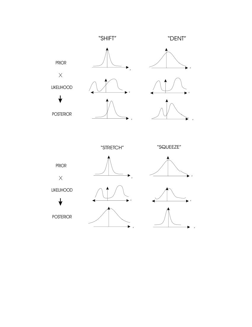
Figure 4.2: Four possible effects of the likelihood factor on a prior distribution

4.6 A Classical System with Dirichlet Boundary Conditions

In the classical description of the measurement, prior knowledge of the reaction variable $x$ becomes entirely relevant when the statistics are analyzed against initial and final conditions imposed on the system. As we have seen so far in this chapter, within a specific, classically post-selected ensemble, the reaction variable parameterizes the effective region in phase-space from which the measured variable $A$ is sampled; in other words, the sampled average of $A$ acquires an implicit $x$ dependence. This dependence is reminiscent of the parametric dependence on $x$ of the local weak value $\alpha(x)$, which we introduced in the previous chapter.

However, the classical analysis also shows that when it comes to the probabilities for the possible values of $x$ over which these $x$-dependent regions are sampled, these are not the probabilities assigned on the basis of our initial preparation of the apparatus. The prior probabilities are re-assessed by a likelihood factor which depends on the posterior sampling volume corresponding to a given value of $x$. This analogy with classical probability re-assessment is still missing within our picture of sampling weak values. Our intention in this section is to pursue the classical analysis one step further in order to establish, both formally and quantitatively, a direct correspondence between the classical and quantum mechanical descriptions of the measurement. In this way we hope to motivate the interpretation of our model.

Now, as we mentioned in the introduction, the idea behind the two-vector formulation is that the full description of the system is contained in the pair of initial and final wave functions. Otherwise, either one of the wave functions tells us only “half of the story”. To pursue the analogy, we shall therefore specialize the analysis of the previous section to a particular set of classical boundary conditions on the system, which can be realized within the quantum mechanical description, and which classically exhibit the property of telling the full story only by their conjunction.

As is well known, in the Hamiltonian Formulation, the trajectory of a system is completely determined by specifying the initial configuration variables $\{q_{i}\}$ and a set of conjugate momenta which can be inverted to yield the initial velocities $\{\dot{q}_{i}\}$. On the other hand, there is also the Lagrangian Formulation, where the trajectory of the system is determined from Dirichlet boundary conditions, in other words, by specifying the values of the $\{q\}$ at two moments in time.

Now, given these conditions, the response of the apparatus is completely determined if in addition one knows the precise value of the reaction variable $x$. On the other hand, if $x$ is uncertain, then further information on the trajectory is needed to precisely determine the response on the apparatus. The available control (or lack of it therefore) on this additional information is what determines the likelihood factor in the posterior probability for $x$. As we shall now see, the conditional response of the apparatus, as well as the likelihood factor, can both be derived from the extremal action function. This will allow us to make a connection with the quantum mechanical situation.

Consider therefore a system described by a single configuration variable $q$, with a free Lagrangian ${\cal L}_{o}(q,\dot{q})$. We assume that all our information about the system consists of its configuration $q_{1}$, at some initial time $t_{1}$, and the configuration $q_{2}$ at some final time $t_{2}$ For simplicity, we shall specialize to the case in which the measured observable is a function of the configuration variable only, i.e.

$$A(\eta)=A(q)\,,$$ (4.40)

measuered at the intermediate time $t_{i}$. This choice affords a considerable simplification as the total Lagrangian is simply the free Lagrangian minus the measurement Hamiltonian:

$${\cal L}(q,\dot{q},t)={\cal L}_{o}(q,\dot{q})+x\delta(t-t_{i})A(q)\,.$$ (4.41)

As before, we disregard the free dynamics of the apparatus.

Now, given the two boundary conditions, the trajectory of the system is completely determined once $x$ is known. The trajectory is the one for which the action functional

$$S[q(t),x]=\int_{t_{1}}^{t_{2}}dt\,{\cal L}_{o}(q,\dot{q})+x\delta(t-t_{i})A(q)$$ (4.42)

is stationary, and thus corresponds to the solution of the Euler- Lagrange equations

$$\frac{\delta S[q(t)]}{\delta q(t)}=\frac{d}{dt}\frac{\partial{\cal L}_{o}}{\partial\dot{q}}-\frac{\partial{\cal L}_{o}}{\partial\dot{q}}-x\delta(t-t_{i})A^{\prime}(q)=0\,$$ (4.43)

subject to the boundary conditions $q(t_{1})=q_{1}$ and $q(t_{2})=q_{2}$. These equations describe the motion of the system under its free evolution, except at the time $t=t_{i}$, where it receives a “kick”, proportional to the gradient of $A$, the intensity and sign of which is given by the reaction variable $x$.

In all fairness, one should note that there may be more than one solution. In fact, one may generally expect this to be the case if $A(q)$ is a non-linear function in $q$ and either $x$ and/or the time $t_{2}-t_{1}$ are not sufficiently small. We shall assume this is not the case, although the extension is interesting in its own right and can be handled without major difficulty.

Supposing then a unique trajectory, the configuration variable of the system as well as every other dynamical variable is completely specified by the initial and final conditions $q_{1}$ and $q_{2}$ and the value of the reaction variable $x$. Let us write this solution as

$$q_{12}(t;x)\,.$$ (4.44)

Note that even if the free evolution is simple, the parametric dependence of the Lagrangian on $x$ and $A(q)$ may generally make this trajectory quite complicated both as a function of $x$ and $t$.

Now, since we know that the pointer variable of the apparatus responds to the function $A(q)$, the response of the pointer variable now becomes an implicit, generally non-linear function of $x$. Let us write this function, somewhat suggestively, as

$$\alpha_{12}(x)=A(q_{12}(t_{i};x))\,.$$ (4.45)

Now define the action functional evaluated at the extremal trajectory as the “extremal action function”

$$S_{12}(x)\equiv S[q_{12}(t;x),x]\,.$$ (4.46)

As it is then easy to show, $\alpha_{12}(x)$ can be obtained from a variation of this function:

$$\alpha_{12}(x)=\frac{dS_{12}(x)}{dx}\,.$$ (4.47)

For this we note that

$$\frac{d}{dx}S[q(tx|q_{1}q_{2}),x]=\int dt\left[\,\frac{\delta S[q(t)]}{\delta q}\frac{dq_{12}(t;x)}{dx}+\delta(t-t_{i})A(q_{12}(t;x))\right]\,.$$ (4.48)

The first term in the brackets is the implicit variation with respect to the trajectory, which vanishes by the Euler-Lagrange equations; thus, what remains is the explicit variation of the action in the second term.

Hence, we observe that once the endpoints of the trajectory are perfectly determined, the classical conditional response of the pointer variable is essentially as if the apparatus had been subject to an effective, impulsive potential

$$V_{eff}=\delta(t-t_{i})S_{12}(x)\,,$$ (4.49)

which then determines a generally non-linear impulse of the pointer variable

$$p_{f}=p_{i}+S_{12}^{\prime}(x)=p_{i}+\alpha_{12}(x)\,.$$ (4.50)

The extent to which this kick is precisely defined now depends exclusively on the extent to which the reaction variable $x$ is controlled.

Suppose therefore that there is some a-priori uncertainty in $x$. To gauge the mechanical effect of the system on the apparatus we must then consider the posterior distribution for the initial state of the apparatus, given the cited boundary conditions on the system. Using Bayes’ Theorem we have

$$dP(xp_{i}|YZ_{s}q_{2}q_{1})=dP(xp_{i}|Y_{a})\frac{dP(q_{2}|xq_{1})}{dP(q_{2}|Y_{a}q_{1})}\,,$$ (4.51)

where we assume no prior dependence of the apparatus on the initial conditions of the system. Next, we compute the Likelihood factor

$$L_{12}(x)=\frac{P(q_{2}|xq_{1})}{P(q_{2}|Y_{a}q_{1})}\,.$$ (4.52)

This is a more delicate computation as the final condition $q_{2}$ is obviously not determined by the initial condition $q_{1}$ and $x$ alone, but rather by the map $q_{2}=q(t_{2},x,q_{1},k_{1})$ where $k_{1}$ is a momentum conjugate to $q_{1}$. In accordance with what was stated earlier, once $x$ becomes uncertain, prior information about the momentum becomes relevant. To find the probability $P(q_{2}|xq_{1})$ we must then assign a-priori probabilities to $k_{1}$. Clearly, knowledge of $x$ and $q_{1}$ entails no knowledge of the initial momentum $k_{1}$. Hence, we appeal to the Gibbs postulate of equal a priori probabilities in phase space consistent with our known information. This assumption poses a slight problem as the momentum is not bounded, but, since we are only interested in likelihood ratios, we may use a limiting sequence of bounded flat distributions, all of which lead to normalizable distributions. When the bounds are taken to infinity,

$$P(q_{2}|xq_{1}) = \int_{k}dP(k|xq_{1})P(q_{2}|xq_{1}k)$$

$$\Rightarrow L_{12}(x) \propto \int dk_{1},\delta(q_{2}-q(x,t;q_{1},k_{1}))\,.$$ (4.53)

Now, with a single extremal solution the integral picks up the value of the momentum $k_{1}$ at $t_{1}$ determined by the extremal solution. What is left after integration is then the Jacobian

$$L_{12}(x)\propto\left|\frac{\partial k_{1}}{\partial q_{2}}\right|\,.$$ (4.54)

Now we use the well-known fact that the extremal action is the generating function of canonical transformations in time [23]. This means that the initial and final momenta defined by the Lagrangian ${\cal L}$ can be obtained from the variation with respect to the initial and final coordinates

$$k_{2}=\frac{\partial S_{12}}{\partial q_{2}}\ \ \ \ k_{1}=-\frac{\partial S_{12}}{\partial q_{1}}\,.$$ (4.55)

Variation of $k_{1}$ with respect to $q_{2}$ then gives us, for the likelihood factor

$$L_{12}(x)\propto\left|\frac{\partial^{2}S_{12}(x)}{\partial q_{1}\partial q_{2}}\right|\equiv\left|\partial_{1}\partial_{2}S_{12}(x)\right|\,.$$ (4.56)

This quantity is well known in Hamilton-Jacobi mechanics [23], it is the so-called Van Vleck determinant or the “density of paths”  [24].

Hence, we observe that in terms of the likelihood factor and the effective impulsive potential, the passive map from the prior initial to posterior final phase-space distributions of the apparatus becomes

$$dP(x,p|YZ_{s};f)=e^{-\pounds_{S_{12}(x)}}\,dP(x,p|Y_{a};i)\,\frac{\left|\partial_{1}\partial_{2}S_{12}(x)\right|}{\int_{x}\,dP(x|Y_{a};i)\,\left|\partial_{1}\partial_{2}S_{12}(x)\right|}\,,$$ (4.57)

and therefore the final distribution of the pointer variable is given by

$$dP(p|YZ_{s};f)=\int_{x}\,dP(x,p-\alpha_{12}(x)\,|Y_{a};i)\,\frac{\left|\partial_{1}\partial_{2}S_{12}(x)\right|}{\int_{x}\,dP(x|Y_{a};i)\,\left|\partial_{1}\partial_{2}S_{12}(x)\right|}\,.$$ (4.58)

We note finally that in this classical example, it is clear what constitutes a mechanical effect of the system on the apparatus— the reversible phase-flow induced by the effective potential, and what constitutes a re-assessment of prior probabilities–the irreversible multiplication by the likelihood factor $\left|\partial_{1}\partial_{2}S_{12}(x)\right|$. This formal distinction will serve as the guiding principle in the interpretation of the non-linear model, to which we now turn.

Chapter 5 The Non Linear Bayesian Model

5.1 Semi-Classical Correspondence

As mentioned earlier, there exist in quantum mechanics initial and final boundary conditions which correspond to conditions that completely determine the microstate of the system in the classical description. One should therefore expect that in a pre-and post-selection with such conditions, and given additional semi-classical conditions where quantum inertial effects may also be neglected on the side of the system, the conditional response of the apparatus should exhibit a correspondence with the classical description of the measurement. We now investigate this correspondence.

Let us then analyze the conditional response of the apparatus, now quantum mechanically, when the system is pre- and post selected on eigenstates of the configuration variable and the measured observable is some function $\hat{A}=A(\hat{q})$ measured at the intermediate time. In this case, using Eq. (2.18) for the relative state of the apparatus we have:

$$|\phi_{f}^{12}\rangle\propto\langle q_{2},t_{2};t_{i}|e^{i\hat{A}\hat{x}}|q_{1},t_{1};t_{i}\rangle\,|\phi_{i}\rangle\,,$$ (5.1)

where the transition amplitude is

$$\langle q_{2},t_{2};t_{i}|e^{i\hat{A}\hat{x}}|q_{1},t_{1};t_{i}\rangle\equiv\langle q_{2}|e^{-i\hat{H}_{o}(t_{2}-t_{i})}\,e^{i\hat{A}\hat{x}}e^{-i\hat{H}_{o}(t_{i}-t_{1})}|q_{1}\rangle$$ (5.2)

and $\hat{H}_{o}$ is the free evolution Hamiltonian of the system. We recognize the transition amplitude as the propagator for the Schrödinger equation for the system with the Hamiltonian $\hat{H}_{o}-\delta(t-t_{i})\hat{A}x$.

Now, it is well known that in the semi-classical regime, i.e., for small times $t_{2}-t_{1}$, and/or to leading order in powers of $\hbar/M$, the solution to the propagator is given by the WKB approximation [24]:

$$\langle q_{2},t_{2};t_{i}|e^{i\hat{A}x}|q_{1},t_{1};t_{i}\rangle_{WKB}\simeq(2\pi i)^{-1/2}\,e^{iS_{12}(x)}\,\sqrt{\left|\partial_{1}\partial_{2}S_{12}(x)\right|}\,,$$ (5.3)

where $S_{12}(\hat{x})$ is the extremal action evaluated at the classical path, and the factor $\partial_{1}\partial_{2}S_{12}(x)$ the classical density of paths, the same terms encountered at the end of the previous chapter. Hence, the state of the apparatus relative to this transition is in the WKB approximation

$$|\phi_{f}^{12}\rangle\propto e^{iS_{12}(\hat{x})}\,\sqrt{\left|\partial_{1}\partial_{2}S_{12}(\hat{x})\right|}|\phi_{i}\rangle\,.$$ (5.4)

Where the phase factor and the square root of the density of paths are now regarded as operator-valued functions of $\hat{x}$. Let us then establish some parallels with the corresponding classical description, i.e., Eq. (4.57)  :

The “Kick”: Consider first the transformation $e^{iS(\hat{x})}$ defined by the phase-factor. Viewing it as an operator-valued function of $\hat{x}$, we note that it is a unitary transformation; hence, as in the classical case, it corresponds to a reversible transformation. Moreover, its effect on the pointer variable operator $\hat{p}$ as seen in the Heisenberg picture, is

$$e^{-iS(\hat{x})}\,\hat{p}e^{iS(\hat{x})}=\hat{p}+\alpha_{12}(\hat{x})\,,$$ (5.5)

which is essentially the “quantized” version of the classical conditional response of the pointer variable, i.e. Eq. (4.50). Now, as we recall, $\alpha_{12}(x)$ in the classical case is the function $A(q)$ evaluated at the trajectory that solves the Euler-Lagrange equations of the system with the measurement back-reaction term. On the other hand, we recall from an earlier discussion that the phase gradient is the local weak value of $\hat{A}$

$$\alpha_{12}(x)={\rm Re}\frac{\langle q_{2},t_{2};t_{i}|\hat{A}e^{i\hat{A}x}|q_{1},t_{1};t_{i}\rangle}{\langle q_{2},t_{2};t_{i}|\,e^{i\hat{A}x}|q_{1},t_{1};t_{i}\rangle}\,,$$ (5.6)

Hence we see that in terms of the equations of motion entailed by the action $S_{12}(x)$, the picture we have so far suggested, namely, that of the pointer responding to the weak value of $\hat{A}$, has a direct classical correspondence. The picture becomes, under semi-classical conditions on the system, the same classical picture in which the pointer variable responds to the value of $A(q)$ on the classical trajectory with measurement back-reaction given a definite value of $x$.

“Sampling”: Consider then the hermitian operator $\sqrt{\partial_{1}\partial_{2}S_{12}(\hat{x})}$ in Eq. (5.4). Computing the normalization of the relative state, we see that the probability distribution for $x$, $dx|\phi_{f}(x)|^{2}$ is given by:

$$dP(x|\phi_{f}^{12})=dP(x|\phi_{i})\frac{\left|\partial_{1}\partial_{2}S_{12}(x)\right|}{\int_{x}\,dP(x|\phi_{i})\,\left|\partial_{1}\partial_{2}S_{12}(x)\right|}\,.$$ (5.7)

where $dP(x|\phi_{i})=dx|\phi_{i}(x)|^{2}$. This expression has exactly the same form as the marginal posterior probability distribution for $x$ obtained in the classical Bayesian analysis, i.e.,

$$dP(x|YZ_{s};f)=dP(x|Y_{a};i)\frac{\left|\partial_{1}\partial_{2}S_{12}(x)\right|}{\int_{x}\,dP(x|Y_{a};i)\,\left|\partial_{1}\partial_{2}S_{12}(x)\right|}\,.$$ (5.8)

In other words, we see that the passage from the initial to the final relative distribution in $x$ in the quantum case, exactly parallels the classical passage from prior to posterior distribution.

Observe therefore that if we define in the quantum case a corresponding likelihood factor as

$$L_{12}(x)\equiv\frac{\left|\partial_{1}\partial_{2}S_{12}(x)\right|}{\langle\phi_{i}|\left|\partial_{1}\partial_{2}S_{12}(x)\right||\phi_{i}\rangle}\,,$$ (5.9)

then the final conditional expectation value of the kick on the pointer variable, i.e.,

$$\langle\phi_{f}^{12}|\,\alpha_{12}(\hat{x})|\phi_{f}^{12}\rangle=\int_{x}dP(x|\phi_{i})L_{12}(x)\,\alpha_{12}(x)\,,$$ (5.10)

can be made to coincide with the posterior expectation value of $\alpha_{12}(x)$ in the classical description. As we recall from the last chapter, in the pre- and post selected classical measurement it is the posterior distribution in $x$ which determines the sampling distribution for $A$. Thus, by identifying the $dP(x|\phi_{i})L_{12}(x)$ as a posterior probability distribution in $x$, the picture of sampling the weak value $\alpha(x)$ also has a direct correspondence with the classical picture of sampling; it corresponds to the sampling of $A(q)$ from regions in the system’s phase-space parameterized by the reaction variable $x$.

“Bias”: Finally, we recall that in the classical case, the systematic effect of the system on the pointer variable is gauged from the posterior average of its initial expectation value. Let us then re-express $|\phi_{f}^{12}\rangle$ as

$$|\phi_{f}^{12}\rangle=e^{iS_{12}(\hat{x})}\sqrt{L_{12}(\hat{x})}\,|\phi_{i}\rangle\,,$$ (5.11)

where we now view the square root of the likelihood factor (5.9) as an operator. If we then look at the expectation value of $\hat{p}$ for the relative state, we find from (5.5) that

$$\langle p_{f}\rangle=\langle\phi_{i}|\sqrt{L_{12}(\hat{x})}\,\hat{p}\,\sqrt{L_{12}(\hat{x})}|\phi_{i}\rangle\,+\langle\phi_{i}|L_{12}(\hat{x})\alpha(\hat{x})|\phi_{i}\rangle.$$ (5.12)

The first term on the right hand side is what corresponds in the classical case to the posterior expectation value of $p_{i}$. Here the parallel is slightly less direct, as $\hat{x}$ and $\hat{p}$ do not commute. Nevertheless, this expectation value still reproduces qualitatively the classical property that if $x$ and $p$ are not independent a-priori, then the posterior expectation value of $p_{i}$ need not coincide with its prior expectation value. The problem of bias is dealt with classically by factoring the phase-space distributions, thus preventing prior correlations between $x$ and $p$. In the quantum case, it is clear that $x$ and $p$ cannot be separated in this way, as the two variables are intrinsically constrained by the uncertainty principle. Nevertheless, it is still possible to establish a general condition to eliminate the bias in the expectation value of $p$, which resembles the classical no-correlation condition. Notice that if the initial wave function $\phi_{i}(x)$ in the $x$ representation can be written as

$$\phi_{i}(x)=R(x)e^{ip_{i}x}\,,$$ (5.13)

where $R(x)$ is a real function of $x$, then since $\sqrt{L_{12}(x)}$ is real as well,

$$\langle\phi_{i}|\sqrt{L_{12}(\hat{x})}\,\hat{p}\,\sqrt{L_{12}(\hat{x})}|\phi_{i}\rangle=\langle\phi_{i}|\hat{p}\,|\phi_{i}\rangle=p_{i}\,.$$ (5.14)

Since the particular choice of $p_{i}$ entails no loss of generality (it only amounts to a redefinition of the momentum reference origin), we shall refer to states for which the wave function in $x$ is of the form (5.13) as “real states”. One can then show that when $|\phi_{i}\rangle$ is a real state, the second order “correlation” function between $\hat{p}$ and any function $f(x)$ which falls of faster than $1/R(x)^{2}$ at infinity,

$$\langle\Delta p\,\Delta f\rangle\equiv\langle\phi_{i}|\,\frac{1}{2}\,\{\hat{p},f(\hat{x})\}\,|\phi_{i}\rangle-p_{i}\langle\phi_{i}|f(\hat{x})|\phi_{i}\rangle=0\,.$$ (5.15)

Thus we see that by imposing a fairly general “no-correlation” condition on the initial state of the apparatus, the systematic effect on the pointer variable can be gauged, both classically and quantum-mechanically, from the same fixed reference origin $p_{i}$. Let us also note in passing an additional desirable feature of real states with regards to bias; if $\phi_{(}x)$ is real, the the real and imaginary parts of its Fourier transform $\phi_{i}(p)$ have definite parities with respect to reflections about the reference origin $p_{i}$; since, therefore, $|\phi_{i}(p)|^{2}$ is symmetric about this origin, any asymmetry in the distribution of the data can be attributed exclusively to the effect of the unitary transformation $e^{iS_{12}(\hat{x})}$.

Now, taking note of the three above parallels, we then draw the following conclusion:

• if the system satisfies the semi-classical conditions, in other words, both in terms of initial and final boundary conditions as well as inertial conditions,

• then the conditional expectation value of $\langle\alpha_{12}(x)\rangle$ can be interpreted, both in the classical and quantum descriptions, as the same systematic effect on the average momentum of the apparatus,

• provided that in the quantum case the “reference” initial quantum state or the apparatus is taken to be the state $\sqrt{L_{12}(\hat{x})}\,|\phi_{i}\rangle\,,$ as opposed to the state $|\phi_{i}\rangle$ that was initially assigned without prior knowledge of the “destiny” of the system.

For the purpose of “calibrating” the model, we shall then make the reasonable assumption that in the classical limit $\hbar/M\rightarrow 0$ on the system, the conditional expectation value corresponds in both descriptions to the same mechanical effect. This leads us then to the formulation of the model under more general non-classical conditions on the system.

5.2 The Model

For any given transition $|\psi_{1}\rangle\rightarrow|\psi_{\mu}\rangle$ of the system, we can write the amplitude function as a real function times a phase

$$\langle\psi_{\mu}|e^{i\hat{A}x}|\psi_{1}\rangle=\sqrt{P(\psi_{\mu}|x\psi_{1})}e^{iS_{\mu}(x)}\,.$$ (5.16)

where $P(\psi_{\mu}|x\psi_{1})$ is the transition probability from $|\psi_{1}\rangle$ to $|\psi_{\mu}\rangle$, given a definite unitary transformation of the system $e^{i\hat{A}x}$; the square root in Eq. (5.16) is allowed to take either sign to ensure continuity in the decomposition. Now, given an initial preparation of the apparatus $|\phi_{i}\rangle$, the relative final state for the apparatus can then be written as

$$|\phi_{f}^{(\mu)}\rangle=e^{iS_{\mu}(\hat{x})}\sqrt{\frac{P(\psi_{\mu}|\hat{x}\psi_{1})}{P(\psi_{\mu}|\phi_{i}\psi_{1})}}\,|\phi_{i}\rangle$$ (5.17)

where we now interpret the normalization factor as the transition probability given this preparation. As we can see, this transition probability satisfies the product rule of probability in the $x$-representation

$$P(\psi_{\mu}|\phi_{i}\psi_{1})=\langle\phi_{i}|P(\psi_{\mu}|\hat{x}\psi_{1})|\phi_{i}\rangle=\int_{x}dP(x|\phi_{i})\,P(\psi_{\mu}|x\psi_{1})\,,$$ (5.18)

and may thus be interpreted, quite intuitively, as the average transition probability when the intermediate transformation is sampled with the initial distribution $dP(x|\phi_{i})$.

Drawing then from the parallel established in the previous section, we now interpret $S(\hat{x})$ as an effective action and infer an underlying action-reaction picture from the unitary operator $e^{iS_{\mu}(\hat{x})}$: for a given transformation on the system system, generated by $\hat{A}$, and parameterized by $x$, there is a corresponding back-reaction on the variable $p$ conjugate to the transformation parameter. The reaction on the apparatus is an impulse proportional to the variation of the action

$$\delta p=S_{\mu}^{\prime}(x)=\alpha_{\mu}(\hat{x})\,.$$ (5.19)

The impulse is then given by

$$\alpha_{\mu}(x)={\rm Re}\frac{\langle\psi_{\mu}|\,\hat{A}\,e^{i\hat{A}x}|\psi_{1}\rangle}{\langle\psi_{\mu}|e^{i\hat{A}x}|\psi_{1}\rangle}\,,$$ (5.20)

the weak value of the generator $\hat{A}$  with parameter value $x$.

Similarly, we infer a probabilistic picture by noting that the irreversible transformation

$$|\phi_{i}\rangle\rightarrow\sqrt{\frac{P(\psi_{\mu}|\hat{x}\psi_{1})}{P(\psi_{\mu}|\phi_{i}\psi_{1})}}\,|\phi_{i}\rangle$$ (5.21)

corresponds, in the $x$-representation, to the square root of a probability re-assessment with the likelihood factor

$$L_{\mu}(x)=\frac{P(\psi_{\mu}|\hat{x}\psi_{1})}{P(\psi_{\mu}|\phi_{i}\psi_{1})}\,.$$ (5.22)

We interpret this factor then as a generalized weight factor which in the semi-classical approximation corresponds to the “density of paths” in phase space. We define therefore a re-assessed initial state of the apparatus according to this “likelihood transformation”

$$|\phi_{i}^{(\mu)}\rangle\equiv\sqrt{L_{\mu}(\hat{x})}|\phi_{i}\rangle\,,$$ (5.23)

denoted then as the initial state of the apparatus relative to the transition $|\psi_{1}\rangle\rightarrow|\psi_{\mu}\rangle$, or the relative initial state for short.

This state will then serve as the “reference frame” in order to gauge the mechanical effect of the system on the apparatus, in accordance with the results of the previous section. Thus, the relative final state is given by

$$|\phi_{f}^{(\mu)}\rangle=e^{iS_{\mu}(\hat{x})}\,|\phi_{i}^{(\mu)}\rangle\,.$$ (5.24)

The distribution of the data may then be analyzed, as in Chapter $2$ within the picture of sampling weak values, i.e., as a superposition of local weak measurements where that instead of $|\phi_{i}\rangle$, we now use the relative initial state $|\phi_{i}\rangle$. The results of that chapter regarding the means and variances of the pointer variable then follow in analogous fashion. We shall concentrate on these in further detail in Sec. (5.6).

Let us for now give a closed-form expression for the conditional probability distribution of the data, following from Eq. (5.24):

$$dP(p|\phi_{f}^{\mu}) = dp\ \langle\phi_{i}^{(\mu)}|\,e^{-iS_{\mu}(\hat{x})}\ \delta(p-\hat{p})\ e^{iS_{\mu}(\hat{x})}\,|\phi_{i}^{(\mu)}\rangle\,$$ (5.25)

$$= dp\ \langle\phi_{i}^{(\mu)}|\ \delta(p-\hat{p}-\alpha_{\mu}(\hat{x})\,)\ |\phi_{i}^{(\mu)}\rangle\,.$$

The expression corresponds then to the “quantized” version of a classical probability model for the data, in which the pointer receives a definite kick $\alpha_{\mu}(x)$ given $x$, and the possible kicks are sampled over the posterior phase-space distribution for the apparatus. We emphasize that the correspondence becomes exact at the level of the expectation value, where assuming a real (i.e., unbiased) initial state of the apparatus with $p_{i}=0$,

$$\langle p_{f}\rangle=\int_{x}dP(x|\phi_{i}^{(\mu)})\alpha_{\mu}(x)=\,\int_{x}dP(x|\phi_{i})L_{\mu}(x)\,\alpha_{\mu}(x)\,;$$ (5.26)

the distribution for $x$ may equivalently be interpreted classically as the the posterior distribution with a likelihood factor $L_{\mu}(x)\propto P(\psi_{\mu}|x\psi_{1})$.

In this way, we fulfill the goal we initially set out for, namely to find an intuitive expression for the distribution of the data, under general conditions of the apparatus, in which the picture of sampling weak values is always at the forefront.

5.3 Interpretation in Terms of the Two-Vector Formulation

Let us briefly discuss some aspects of interpretation surrounding the three elements of our model.

5.3.1 The Sampled States

According to the two vector formulation, at any given moment in time an initial and final vector are needed describe the system. What corresponds then to the “state”, i.e., analogous to the point in phase-space, is a pair of vectors in Hilbert space. In the model, the idea is therefore that by varying the parameter $x$ we move from one pair to another. It is important then to note what these pairs are.

Let us recall that in the classical situation considered at the end of the last chapter, when one fixes the end-points of the configuration variable trajectory, the whole trajectory becomes dependent on $x$. In particular, the phase-space points $(q_{i},k_{i})$ and $(q_{f},k_{f})$ are $x$ -dependent. These points are then connected by the canonical transformation generated by the measured function $A(q)$ with parameter $x$, i.e.,

$$q_{f}(x)=q_{i}(x)\,,\ \ \ \ p_{f}(x)=p_{i}(x)+xA^{\prime}(q)\,.$$ (5.27)

Here we have a similar situation. Denoting by $\omega(x)$ a pair of vectors at a given time, the description is given by the point

$$\omega_{i}(x)=\left(\,|\psi_{1}\rangle\,,\,e^{-i\hat{A}x}|\psi_{\mu}\rangle\,\right)$$ (5.28)

immediately before the measurement interaction, and by the point

$$\omega_{f}(x)=\left(\,e^{\hat{A}x}|\psi_{1}\rangle\,,\,|\psi_{\mu}\rangle\,\,\right)$$ (5.29)

immediately after. The mechanical transformation of the system via back-reaction is then the map from the point $\omega_{i}(x)$ to the point $\omega_{f}(x)$ in the space of vector pairs, which is generated by the unitary operator $e^{i\hat{A}x}$:

$$\omega_{f}(x)=\left(\,e^{i\hat{A}x}\,,e^{i\hat{A}x}\,\right)\,\omega_{i}(x).$$ (5.30)

A way of seeing this is to consider giving a finite time duration $T$ to the measurement of $\hat{A}$, and in between, at some time $\epsilon T$ (with $\epsilon<1$) after the interaction is switched on, insert an impulsive but very weak measurement of some other observable $\hat{B}$ that does not commute with $A$. In this case the parametric dependence of the amplitude function is on two variables, $x$, and the reaction variable of the other apparatus, call it $y$:

$$\langle\psi_{\mu}|e^{i\hat{A}(1-\epsilon)x}e^{i\hat{B}y}e^{i\hat{A}\epsilon x/2}|\psi_{1}\rangle\,.$$ (5.31)

Concentrating then on a fixed value of $x$, the weak value of $\hat{B}$ at the point of no-reaction, $y=0$, is then

$${\rm Re}\frac{\langle\psi_{\mu}|e^{i\hat{A}(1-\epsilon)x}\hat{B}e^{i\hat{A}\epsilon x}|\psi_{1}\rangle}{\langle\psi_{\mu}|e^{i\hat{A}x}|\psi_{1}\rangle}\,.$$ (5.32)

Thus we see that by moving from $\epsilon=0$ to $\epsilon=1$, the weak value of $\hat{b}$ changes from that evaluated at $\omega_{i}(x)$ to that evaluated at $\omega_{f}(x)$.

5.3.2 Weak Values

We also saw how in the semi-classical picture, the weak value of the operator $A(\hat{q})$ is the function $A(q)$ evaluated at the classical trajectory given $x$; hence, at the point of no reaction $x=0$, $A(q)$ is evaluated at the free trajectory, and so, for instance, the weak value of say $\hat{q}^{2}$ will be equal to the weak value of $\hat{q}$, squared. In general, however, this shall not be the case. Not only will the weak values of $\hat{A}^{2}$ and the square of the weak value of $\hat{A}$ differ in general, but moreover the weak value of $\hat{A}^{2}$ need not be positive.

In this respect, it is important to note that weak values are defined operationally as the response to an almost-perfect unitary transformation generated by the observable $\hat{A}$; hence, one should not expect a priori any particular relation between the weak values of two operators that have a common spectral decomposition, as they may lead to entirely different transformations. It is therefore more convenient to think of weak values in terms of the algebra of generators of unitary transformations, where $\hat{A}$ and $\hat{A}^{2}$, although having common eigenvalues, may nevertheless be linearly independent. Note for instance that for a spin-$1/2$ particle, the operators $\hat{S}_{x}^{2}$ , $\hat{S}_{y}^{2}$ and ${S}_{z}^{2}$ are equivalent to the unit matrix. Therefore, they are generators of a trivial unitary transformation, namely an overall phase change. On the other hand, the square of the weak value of $\hat{S}_{x}$, a generator of rotations, may take arbitrarily large values.

5.3.3 Relative Initial State

The interpretation of the relative initial state $|\phi_{i}^{(\mu)}\rangle$ as a sort of posterior initial quantum state is admittedly a more delicate matter. As we argued at the beginning of the chapter, this choice is practically determined by the semi-classical approximation on the system in order to interpret the average shift in the momentum as the same effect both in the classical and quantum descriptions of the apparatus. Furthermore, we have also found it a very convenient way of analyzing the response of the apparatus, as we shall do in the next chapter, if the emphasis is placed on the reaction variable $x$ as we have done all along. The intuition comes precisely because of the fact that in the $x$-representation, the likelihood transformation can then be interpreted in terms of classical probability.

One may nevertheless wonder if a more direct connection to probability can be established for the state $|\phi_{i}^{(\mu)}\rangle$ within the two-vector formulation. For this we note that if only an initial vector is given, then there are an infinite possibility of final states to fill the missing slot. Hence the standard quantum state according to the two-vector description automatically

Thus for instance, if a post-selection is performed on the apparatus in a given basis $B=\{|\chi_{\nu}\rangle\}$, the weak values $\tau$ of some apparatus observable $\hat{T}$ are distributed according to

$$dP(\tau|\phi_{f}^{(\mu)}B)=d\tau\,\sum_{\nu}\|\langle\chi_{\nu}|\phi_{f}^{(\mu)}\rangle\|^{2}\delta\left(\tau-{\rm Re}\frac{\langle\chi_{\nu}|\hat{T}|\phi_{f}^{(\mu)}\rangle}{\langle\chi_{\nu}|\phi_{f}^{(\mu)}\rangle}\right)\,.$$ (5.33)

The mean value of this distribution, as one can then verify, is

$$\overline{\tau_{f}}=\langle\phi_{f}^{(\mu)}|\hat{T}|\phi_{f}^{(\mu)}\rangle\,,$$ (5.34)

the standard expectation value.

One may then ask how this works with the same post selection, but for the weak value of $\hat{T}$ at some time, a) before the measurement interaction, and b) after some prior determination of the actual initial state $|\phi_{i}\rangle$. In this case one obtains a distribution similar to Eq. (5.33), except that the weak values in the argument of the delta function are now

$$\tau_{\nu,i}={\rm Re}\frac{\langle\chi_{\nu}|\sqrt{P(\psi_{\mu}|\hat{x}\psi_{1})}e^{iS_{12}(\hat{x})}\hat{T}|\phi_{i}\rangle}{\langle\chi_{\nu}|\sqrt{P(\psi_{\mu}|\hat{x}\psi_{1})}e^{iS_{12}(\hat{x})}|\phi_{i}\rangle}$$ (5.35)

with the same weights as before. The summation cannot be worked out any further than Eq. (5.33) without additional knowledge of the final basis. However, it is still possible to see two indications that the relative state $|\phi_{i}\rangle$ does convey some statistical information about the state of the apparatus before the interaction, if by this information we mean averages of weak values:

First, when $\hat{T}$ is any operator function of $\hat{x}$, $T(\hat{x})$, one can easily see that the weak values coincide both before and after the measurement interaction. This should not be too surprising as $\hat{x}$ is a constant of the motion. Noting therefore that

$$\langle\phi_{f}^{(\mu)}|T(\hat{x})|\phi_{f}^{(\mu)}\rangle=\langle\phi_{i}^{(\mu)}|T(\hat{x})|\phi_{i}^{(\mu)}\rangle\,,$$ (5.36)

we see that given any basis of post-selection on the apparatus, the average weak value of $T(\hat{x})$ before the interaction is given by its standard expectation value given the relative initial state $|\phi_{i}^{(\mu)}\rangle$.

Secondly, when $\hat{T}$ is not a function of $x$, one can still find a simple basis-independent expression for the average weak value before the interaction, namely:

$$\overline{\tau_{i}} = {\rm Re}\frac{\langle\phi_{i}|P(\psi_{\mu}|\hat{x}\psi_{1})\hat{T}|\phi_{i}\rangle}{\langle\phi_{i}|P(\psi_{\mu}|\hat{x}\psi_{1})|\phi_{i}\rangle}$$ (5.37)

$$= \langle\phi_{i}^{(\mu)}|\hat{T}|\phi_{i}^{(\mu)}\rangle+{\rm Re}\langle\phi_{i}^{(\mu)}|\ [\ \sqrt{L_{\mu}(\hat{x})}\,,\,\hat{T}\ ]\ |\phi_{i}\rangle$$

The expression differs from the expectation value of $\hat{T}$ given the initial relative state $|\phi_{i}^{(\mu)}\rangle$ by additional term involving the likelihood factor, the significance of which is unclear at this point. Nevertheless, one easily notes then when $\hat{T}$ is the pointer variable operator $\hat{p}$ itself,

$${\rm Re}\langle\phi_{i}^{(\mu)}|\ [\ \sqrt{L_{\mu}(\hat{x})}\,,\,\hat{p}\ ]\ |\phi_{i}\rangle={\rm Im}\,\langle\phi_{i}^{(\mu)}|\ \frac{L^{\prime}_{\mu}(\hat{x})}{L_{\mu}(\hat{x})}|\phi_{i}^{(\mu)}\rangle=0\,.$$ (5.38)

This is an entirely satisfying result as it then shows that the reference origin for the “kick”, i.e.,

$$\langle p_{i}\rangle=\langle\phi_{i}^{(\mu)}|\hat{p}|\phi_{i}^{(\mu)}\rangle\,$$ (5.39)

indeed corresponds to an average of the momentum operator, in this case its average weak value, immediately before the interaction occurred.

5.4 Connection with Likelihood Factor

We shall now turn to more practical considerations regarding the model. As we have seen, forefront in the picture of sampling weak values is the distribution for the reaction variable $x$. As should be clear then, the distribution of interest is the posterior distribution

$$dP(x|\phi_{i}^{\mu})=dP(x|\phi_{i})\,L_{\mu}(x)\,$$ (5.40)

and not its prior distribution, as in the classical situation. It is then this distribution, in which the Likelihood factor plays a decisive role, which defines then the appropriate conditions under which the model may be linearized. Also, away from the weak regime, we saw in Chapt. $2$ how the mean and variance of the data are connected to the distribution in $x$. We have already seen how the mean is connected to the posterior distribution. What remains therefore is to establish the connection in the variance. In the following two sections we shall then consider the recovery of the linear model in the weak regime and the general connection between the “error laws” and the posterior distribution in $x$. Before doing so, a cautionary remark is in order:

As its name implies, the non-linearity in the model stems from the fact that the response of the pointer variable is now seen as an impulse in $x$ which is generally a non-linear function $\alpha_{\mu}(x)$. Such a model could be separated in classical mechanics if $x$ and $p$ were initially uncorrelated; in that case then, the model could be turned back into a linear model by a trivial redefinition of the variables, i.e. $A=\alpha(x)$. Clearly, such is not the case in the quantum version, as $\hat{p}$ and $\alpha_{\mu}(\hat{x})$ satisfy the commutation relation $[\hat{p}\,,\alpha_{\mu}(\hat{x})]=-i\alpha_{\mu}^{\prime}(\hat{x})\neq 0$.

The idea of sampling in the statistical sense must then be taken with some caution when dealing with the overall shape of the pointer variable distribution. One should keep in mind that the basic object is always the wave function

$$\phi_{f}^{(\mu)}(p)=\frac{1}{\sqrt{2\pi}}\int_{-\infty}^{\infty}dx\,\sqrt{L_{\mu}(x)}\,\phi_{i}(x)e^{iS_{\mu}(x)-ipx}$$ (5.41)

from which the conditional probability distribution is derived. The sampling should hence be understood in the sense of Chapter $2$, by considering the wave function as a coherent superposition of narrow samples, each of which if narrow enough may then be treated as being shifted by the local weak value. The point then is that the elements of the superposition also carry phase information and hence the interference between the samples will show up in modifications to the moments of the pointer variable distribution which are higher than the first moment.

5.5 Recovery of The Weak Linear Model

Let us then consider the conditions for the recovery of the the WLM as the model “sharpens” with $x$ to the point where a single weak value is sampled. This occurs when the magnitude of the relative initial wave function $\phi_{i}^{(\mu)}(x)=\sqrt{L_{\mu}(x)}\,\phi_{i}(x)$ is sharply peaked around a value $x_{\mu}$, in which case we can apply a “group velocity” approximation to Eq. (5.41) as in Chapter $2$. A necessary condition for this is then that the nonlinear terms in the phase expansion $\alpha^{\prime}_{\mu}(x_{\mu})(x-x_{\mu})^{2}+\,...$ may be neglected. Hence, assuming $\alpha^{\prime}_{\mu}(x_{\mu})$ is not too small compared to the higher order terms, we demand that

$$\alpha^{\prime}_{\mu}(x_{\mu})\Delta x^{2}\ll 1\,.$$ (5.42)

In passing, we note that the gradient $\alpha^{\prime}_{\mu}(x)$ of the local weak value may also be expressed in terms of the imaginary part of a complex variance-like quantity, namely

$$\alpha^{\prime}(x)=-{\rm Im}\left[\ \frac{\langle\psi_{\mu}|\hat{A}^{2}e^{i\hat{A}x_{\mu}}|\psi_{1}\rangle}{\langle\psi_{\mu}|e^{i\hat{A}x_{\mu}}|\psi_{1}\rangle}-\frac{\langle\psi_{\mu}|\hat{A}e^{i\hat{A}x_{\mu}}|\psi_{1}\rangle}{\langle\psi_{\mu}|e^{i\hat{A}x_{\mu}}|\psi_{1}\rangle}^{2}\ \right]\,,$$ (5.43)

as can be shown with relative ease.

Let us suppose that $S(x)$ can be expanded in a Taylor series around $x_{\mu}$ up to the linear terms in $(x-x_{\mu})$. The final wave function is then a rigid translation of the Fourier transform $\phi_{i}^{(\mu)}(p)$

$$\phi_{f}^{(\mu)}(p)\simeq e^{iS(x_{\mu})-i\alpha_{\mu}(x_{\mu})x_{\mu}}\,\phi_{i}^{(\mu)}(p-\alpha_{\mu}(x_{\mu}))\,$$ (5.44)

where the translation is the local weak value evaluated at $x_{\mu}$. Thus we recover in the resulting conditional distribution the statistically separable form under the WLM

$$dP(p\,|\phi_{f}^{(\mu)})\simeq dP(p-\alpha(x_{\mu})|\phi_{i}^{(\mu)})\,,$$ (5.45)

where a single weak value is sampled. It is important to note two generalizations from the WLM as discussed in Chapt. 1. First is the obvious generalization to a different “sampling” point $x_{\mu}$ away from $x=0$, as we saw in Chapt. $2$. More important now is the fact that what determines the linearity condition is the relative initial state $|\phi_{i}^{(\mu)}\rangle$ and not the initial state $|\phi_{i}\rangle$; hence; the probability distribution that gets shifted is not in general $dP(p|\phi_{i})$ but rather $dP(p|\phi_{i}^{(\mu)})$. This leads us then to consider the conditions on the Likelihood factor under which “sharpness in $x$” is achieved.

For this we may concentrate on the probability distribution as opposed to the amplitude, and draw the intuition from the classical situation described earlier. Similarly to what we saw there, it is the interplay between the prior $dP(x|\phi_{i})$ and the likelihood factor $L_{\mu}(x)$ that ultimately determines whether a weak regime of sharp $x$ is achieved or not. Here, the condition that $dP(x|\phi_{i})$ is “sufficiently sharp” around some value $x_{o}$, say that $\Delta x$ be small compared to $|\alpha(x_{\mu})/\alpha^{\prime}_{\mu}(x_{\mu})|$, may not be enough to guarantee that the posterior distribution $dP(x|\phi_{i})L_{\mu}(x)$ will be sharp as well. It could happen, for instance, that the transition probability $P(\psi_{\mu}|x\psi_{1})$ in the likelihood factor has a minimum at $x_{o}$ and rises so fast that the posterior distribution is considerably widened or “dented”, as in Fig. (4.2). Or, it could be that somewhere around the tail regions of $dP(x|\phi_{i})$, the transition probability $P(\psi_{\mu}|x\,\psi_{1})$ becomes overwhelmingly large. In that case, the mass of the distribution shifts to that region where the values of $x$ are most favorable to the transition.

If one is therefore interested in probing the local weak value close to some point $x_{o}$, the “probe” $dP(x|\phi_{i})$ needs to be sufficiently robust against the likelihood factor (see Fig. 5.1). It is important to note in this respect that unless the support of $dP(x|\phi_{i})$ is completely severed outside the region of interest, the robustness condition is generally a global condition if $dP(x|\phi_{i})$ has tails stretching out to infinity. However, as the transition probability $P(\psi_{\mu}|x\psi_{1})$ can never exceed unity anywhere, robustness can always be achieved by imposing a sufficiently fast fall-off rate of $dP(x|\phi_{i})$ outside the region of interest.

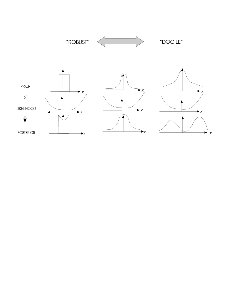
Figure 5.1: Robustness/docility of three prior distributions against the likelihood factor. A relatively sharp prior may not be sufficiently robust to ensure that the posterior distribution is sharp as well, if for instance, its rate of fall-off is faster than the rise rate of the likelihood factor.

Now, assuming that the prior is then both sharp and robust against the likelihood factor, the leading order effect of the latter should be should then be a small “shift” towards regions in $x$ favorable to the transition, similar to the one illustrated in Fig. 4.2. The resulting “sampling point” point $\equiv x_{\mu}$, or point of maximum likelihood produced by this bias, may then be interpreted as the most likely value of $x$ at which the transition occurred. In other words, we view the system as suffering a “back-reaction” $\simeq e^{i\hat{A}x_{\mu}}$.

To a leading approximation, this sampling point may be obtained by a Taylor expansion of $L_{\mu}(x)$ about $x_{o}$ and keeping the first-order term. Now, if one writes the complex local weak value $A_{w}^{(\mu)}(x)$ as

$$\frac{\langle\psi_{\mu}|\hat{A}e^{i\hat{A}x_{\mu}}|\psi_{1}\rangle}{\langle\psi_{\mu}|e^{i\hat{A}x_{\mu}}|\psi_{1}\rangle}=\alpha_{\mu}(x)+i\beta_{\mu}(x)\,,$$ (5.46)

it is then easy to see that the first derivative of the log-likelihood factor is

$$\frac{\partial}{\partial x}\log L_{\mu}(x)=-2\beta_{\mu}(x).$$ (5.47)

where $\beta_{\mu}(x)$ is the imaginary part of the complex local weak value $A_{w}^{(\mu)}(x)$; thus, one may approximate $L_{\mu}$ locally as

$$L_{\mu}(x)\propto e^{-2{\rm Im}\,A_{w}^{(\mu)}(x_{o})(x-x_{o})}\ .$$ (5.48)

If $dP(x|\phi_{i})$ then satisfies a sufficiently rapid fall-off condition, then the exponential approximation of Aharonov and Vaidman is valid and the shift can be viewed as an imaginary shift of the initial wave function $\phi_{i}(x)$ by the imaginary part of the weak value. This produces to leading order a shift from the a priori sampling point $x_{o}$ of approximately

$$x_{\mu}\simeq x_{o}-2\,\Delta x^{2}\,{\rm Im}\,A_{w}^{(\mu)}(x_{o})\,,$$ (5.49)

and in turn this provides an operational interpretation of the imaginary part of the weak value.

However, the idea of a sharply defined sampling point may be inadequate, for example, if the posterior distribution is considerably wider than the initial distribution but the the weak regime can still be achieved (i.e., slowness of $\alpha(x)$). In such case, corrections to the width in $x$ must be taken into account. In the case of a Gaussian packet, the leading correction to the width in $x$ in the Gaussian approximation is easily obtained:

$$\sigma_{\mu}\simeq\frac{\sigma}{\sqrt{1+2\sigma^{2}\,\beta^{\prime}(x_{\mu})}}\,.$$ (5.50)

We note that similarly to the case of the real part of the complex weak value in Eq. (5.43), the gradient $\beta^{\prime}(x)$ is given in terms of the real part of the same variance-like quantity, i.e.,

$$\beta^{\prime}(x)={\rm Re}\left[\ \frac{\langle\psi_{\mu}|\hat{A}^{2}e^{i\hat{A}x_{\mu}}|\psi_{1}\rangle}{\langle\psi_{\mu}|e^{i\hat{A}x_{\mu}}|\psi_{1}\rangle}-\frac{\langle\psi_{\mu}|\hat{A}e^{i\hat{A}x_{\mu}}|\psi_{1}\rangle}{\langle\psi_{\mu}|e^{i\hat{A}x_{\mu}}|\psi_{1}\rangle}^{2}\ \right]\,.$$ (5.51)

These expressions, in conjunction with Eq. 5.43, also determine that (and as already seen in Chapter $2$)

$$\left\|\frac{\langle\psi_{\mu}|(\hat{A}-A_{w})^{2}|\psi_{1}\rangle}{\langle\psi_{\mu}|\psi_{1}\rangle}\right\|\Delta x^{2}\ll 1\,$$ (5.52)

is a necessary local condition which, in addition to the global robustness condition, guarantees that the response of the apparatus can be described in terms of a complex shift by $\frac{\langle\psi_{\mu}|\hat{A}|\psi_{1}\rangle}{\langle\psi_{\mu}|\psi_{1}\rangle}$ of the initial wave function in the $p$-representation (here assuming that the sampling point $\simeq 0$).

5.6 Error Laws

We now turn to the connection between the likelihood factor and the “error law” for the conditional distribution $dP(p\,|\phi_{f}^{(\mu)})$, for which we now assume that the variance exists. Assuming for simplicity a real state with $p_{i}=0$, the variance is then given by

$$\Delta{p}_{f}^{2}=\langle\phi_{i}^{(\mu)}|\hat{p}^{2}|\phi_{i}^{(\mu)}\rangle+\Delta\alpha_{\mu}^{2}\,,$$ (5.53)

where $\Delta\alpha_{\mu}^{2}$ is the variance of the local weak with respect to the posterior distribution in $x$ and demands no explanation. On the other hand, it is in the variance of $\hat{p}$ in the first term where we begin to see differences between the classical and quantum mechanical probability models for the apparatus. As mentioned earlier, classically one can completely eliminate the correlations between $p$ and $x$ in the posterior initial distribution. In such case the posterior initial variance in $p$ remains the same as its prior. On the other hand, this cannot happen quantum mechanically as it would lead to a violation of the uncertainty principle, if for instance the posterior distribution in $x$ is narrower than its prior.

To see therefore what the effect of the likelihood factor is on the initial variance, let us assume that both the likelihood factor and $\phi_{i}(x)$ are twice-differentiable. Now define for a given probability distribution a “quadrature” $Q(x)$

$$Q(x)\equiv-\frac{\partial^{2}}{\partial x^{2}}\log\frac{dP(x)}{dx}\,$$ (5.54)

so that for instance a a normal distribution has a constant quadrature $1/\sigma^{2}$. the r.h.s. are the corresponding expectation values of $\hat{p}$ and $\alpha(\hat{x})$ taken with the reference state $|\phi_{i}^{(\mu)}\rangle$. We the have, for the posterior distribution a quadrature

$$Q_{\mu}(x)=Q_{i}(x)+2\beta^{\prime}(x)$$ (5.55)

where $Q_{i}(x)$ is the quadrature of $dP(x\,|\phi_{i})$. For a real state then, one can easily show that

$$\langle\hat{p}^{2}\rangle=\frac{1}{4}\langle\,Q(x)\rangle\,.$$ (5.56)

Hence we can recast (5.53) as the “error law”

$$\Delta p^{2}_{f}=\frac{1}{4}\,\langle Q_{i}(x)\,\rangle+\frac{1}{2}\langle\,\beta^{\prime}(x)\,\rangle+\langle\Delta\alpha_{\mu}^{2}(x)\rangle\,,$$ (5.57)

where now all averages can be taken with respect to the posterior distribution in $x$.

Noting then that for the initial state the average of $\hat{p}^{2}$ is the first term $\frac{1}{4}\,\langle Q_{i}(x)\,\rangle$, but averaged over $dP(x|\phi_{i})$, we see that there is a sense in which real Gaussian states may be regarded as the least biased of test functions, for in that case the average $\langle Q_{i}(x)\,\rangle$ coincides both in the prior and posterior cases, and one then has:

$$\Delta p^{2}_{f}=\Delta p^{2}_{i}+\frac{1}{2}\langle\,\beta^{\prime}(x)\,\rangle+\langle\Delta\alpha_{\mu}^{2}(x)\rangle\,,$$ (5.58)

where $\Delta p^{2}_{i}$ is the variance with respect to the initial Gaussian state. In that case then one may interpret the error law as the contribution of three terms: the initial noise plus the variance in the sampled weak values plus an additional correction to the width due to the likelihood factor.

Let us now see what happens when the posterior distribution in $x$ becomes sufficiently narrow about a sampling point $x_{\mu}$. In that case, the uncertainty in the weak value may be disregarded altogether, and the average of $\beta^{\prime}(x)$ may be replaced by its value at the sampling point. Assuming an initial Gaussian state, we then have the “error law” for weak measurements:

$$\Delta p_{f}^{2}=\Delta p_{i}^{2}+\frac{1}{2}\,\beta^{\prime}(x_{\mu})\,.$$ (5.59)

This expression may be cast in a slightly more intuitive form by recalling from Eq. 5.51 that $\beta^{\prime}(x_{\mu})$ may be expressed in terms of a variance-like quantity. However, the formal similarity to a true error law where this quantity is viewed as something of a “weak uncertainty” should not be pursued too much. For one, the factor of $1/2$ has no place in such error law, at least in a linear model. More importantly, however, is an interesting consequence of the fact that “likelihood in $x$ has effects in $p$”:

Suppose that the likelihood factor is a minimum at the sampling point so that $\beta(x_{\mu})=0$ and $\beta^{\prime}(x_{\mu})<0$. In that case then one should see a “stretch/squeeze” effect: a decrease in the variance with respect to that of the initial distribution, an effect which of course would be impossible to understand classically if $x$ and $p$ were assumed to be uncorrelated a priori.

The “stretch/squeeze” effect is characteristic of the weak regime only. Since the transition probability $P(\psi_{\mu}|x\psi_{1})$ can never exceed unity, it is guaranteed that if the likelihood factor has a local minimum, then it must also have at least two local maxima, perhaps at infinity, where $\beta^{\prime}\geq 0$. Since in the strong regime the prior distribution in $x$ will be docile with respect to the likelihood factor, then the predominant contribution to $\langle\beta^{\prime}\rangle$ will come from precisely those regions of maximal likelihood where $\beta^{\prime}>0$. An illustration of the “stretch/squeeze” effect will be given in the next chapter.

5.6.1 Pooling The Data

Using the results of the the previous section, we finish this chapter by seeing then how the standard error laws of the unconditional distribution, i.e.,

$$\langle p\rangle_{f} = \langle\psi_{1}|\hat{A}|\psi_{1}\rangle$$

$$\Delta p_{f}^{2} = \Delta p_{i}^{2}+\langle\psi_{1}|\Delta\hat{A}^{2}|\psi_{1}\rangle\,;$$ (5.60)

are recovered in the “pooling” of the data from all the post-selected sub-samples. For simplicity we assume an initial Gaussian state with $p_{i}=0$. The sum rule for the expectation value is simple enough. With the bar-average, weighted with the transition probabilities $P(\psi_{\mu}|\phi_{i}\psi_{1})=P(\psi_{\mu}|\Psi_{f})$, one clearly has

$$\overline{\langle p_{f}\rangle}=\overline{\langle\alpha\rangle}\,=\langle\psi_{1}|\hat{A}|\psi_{1}\rangle.$$ (5.61)

The standard average can then be interpreted as a double average of the weak values, first over $x$ given a specific transition, then as average over all transitions. For the variance, we need the conditional averages of $p_{f}^{2}$, which are then given by

$$\langle p_{f}^{2}\rangle=\langle p_{i}^{2}\rangle+\frac{1}{2}\langle\beta^{\prime}\rangle+\langle\alpha^{2}\rangle\,,$$ (5.62)

and from this we then obtain:

$$\overline{\langle p_{f}^{2}\rangle}-\overline{\langle p_{f}\rangle}^{2}=\langle p_{i}^{2}\rangle+\frac{1}{2}\overline{\langle\beta^{\prime}\rangle}+\overline{\langle\alpha^{2}\rangle}-\overline{\langle\alpha\rangle}^{2}\,$$ (5.63)

comparing then with the expression for the variance in the unconditional distribution, we see that

$$\langle\psi_{1}|\Delta\hat{A}^{2}|\psi_{1}\rangle=\frac{1}{2}\overline{\langle\beta^{\prime}\rangle}+\overline{\Delta\alpha^{2}}+\overline{\langle\alpha\rangle^{2}-\overline{\langle\alpha\rangle}^{2}}\,.$$ (5.64)

The rightmost two terms are easy to understand: one is the average variance of $\alpha$ over all sub-samples, the other the scatter in the sub-sample averages. It is interesting to note however that neither of these two terms yields an expression that is independent of the final basis; in other words, the scatter in the weak values generally carries a trace of the final choice of measurement. The trace is “covered” by the first average squeeze term.

Finally, let us turn to the pooling of the errors in the case of weak measurements. For simplicity let us take a Gaussian prior in the limit $\Delta x\rightarrow 0$. Let us also assume that for all transitions, $\langle\psi_{\mu}|\psi_{1}|^{2}\neq 0$ and robustness so that the sampling point tends to $x=0$ for all transitions as $\Delta x\rightarrow 0$. We thus take the weights to be the unperturbed weights $|\langle\psi_{\mu}|\psi_{1}|^{2}$ and neglect the dispersion in $\alpha$, in such case Eq.(5.64) simplifies to

$$\langle\psi|\Delta\hat{A}^{2}|\psi\rangle=\frac{1}{2}\overline{\beta^{\prime}}+\overline{\alpha^{2}-\overline{\alpha}^{2}}\,,$$ (5.65)

where for each transition we take $\alpha_{\mu}={\rm Re}\frac{\langle\psi_{\mu}|\hat{A}|\psi_{1}\rangle}{\langle\psi_{\mu}|\psi_{1}\rangle}$ and

$$\beta_{\mu}^{\prime}={\rm Re}\left[\ \frac{\langle\psi_{\mu}|\hat{A}^{2}|\psi_{1}\rangle}{\langle\psi_{\mu}|\psi_{1}\rangle}-\frac{\langle\psi_{\mu}|\hat{A}|\psi_{1}\rangle}{\langle\psi_{\mu}|\psi_{1}\rangle}^{2}\ \right]\,.$$ (5.66)

The above gives therefore an interpretation of the increase in the variance in the unconditional distribution as made up of both the scatter in the weak values, and the average effect on the widths of the initial distributions. It is also worth noting another, less operational interpretation of the unconditional variance in terms of the transition variances of the real and imaginary parts of the weak value. Noting that the bar- average of $\beta={\rm Im}\frac{\langle\psi_{\mu}|\hat{A}|\psi_{1}\rangle}{\langle\psi_{\mu}|\psi_{1}\rangle}$ vanishes, it is then easily verified that [25]

$$\langle\psi|\Delta\hat{A}^{2}|\psi\rangle=\overline{\alpha^{2}-\overline{\alpha}^{2}}+\overline{\beta^{2}-\overline{\beta}^{2}}\,.$$ (5.67)

As the expression is now written as the sum of positive-definite quantities for each transition, as opposed to Eq. (5.65), we obtain the general result that the scatter in $\alpha$ around $\langle\psi|\hat{A}|\psi\rangle$ is always smaller than the uncertainty $\sqrt{\langle\psi|\Delta\hat{A}^{2}|\psi\rangle}$.

Chapter 6 The Non-Linear Model in Action

6.1 Eccentric Weak Values and Super Oscillations

According to the results at the end of the last chapter, for a pre-selected sample the uncertainty in $\alpha$ around the standard expectation value is always smaller or equal to the standard variance. Thus, one is to expect that for the overwhelming majority of boundary conditions, the weak value of $\hat{A}$ will not show significant deviations from the range of expectation defined by the spectrum of $\hat{A}$. The “pearls” of weak measurements are, however, those exceptional circumstances where the conditional expectation value lies outside, perhaps significantly outside, this prior region of expectation. As we saw in Chapter $2$, these effects could be understood in the representation of the pointer variable as a curious interference phenomenon, whereby wave functions shifted by the eigenvalues of $\hat{A}$ interfere destructively in the “normal” region and somehow, almost magically, interfere constructively at the location determined by the weak value.

On the other hand, as we have argued within the model, the real part of the weak value corresponds to a unitary transformation defined by the phase of the transition amplitude $\langle\psi_{\mu}|e^{i\hat{A}x}|\psi_{1}\rangle$, a transformation that becomes a definite kick to the same extent to which $x$ becomes definite in its posterior distribution. The “magic” must therefore be related to an anomalous behavior of the amplitude function around the sampled region, and, in particular, of the phase factor. This little known phenomenon in Fourier analysis is known as that of of super-oscillations: a synthesis of Fourier modes which locally exhibits an oscillation frequency outside of its Fourier spectrum [26, 27]. Let us now look at a simple way of generating such functions.

6.1.1 N-spins

For concreteness, consider first what turns out to be in fact a rather innocuous example: a single spin-$1/2$ particle pre-and post-selected in eigenstates $|\!-\!\gamma/2\rangle$ and $|\gamma/2\rangle$ of

$$-\sin\left(\frac{\gamma}{2}\right)\hat{S}_{x}+\cos\left(\frac{\gamma}{2}\right)\hat{S}_{z} = 1/2$$

$$\sin\left(\frac{\gamma}{2}\right)\hat{S}_{x}+\cos\left(\frac{\gamma}{2}\right)\hat{S}_{z} = 1/2\,,$$ (6.1)

respectively, and an intermediate measurement of $\hat{A}=\hat{S}_{z}$. When $\gamma=\pi/2$ this is the situation described in the introductory chapter, where the weak value of $\hat{A}$ is the vector sum of the initial and final spin directions, i.e., $\frac{1}{\sqrt{2}}$. For other values of $\gamma$, the weak value of $\hat{A}$ at $x=0$, is easily computed by adding the two “constraint” equations (6.1.1) and “solving” for $\hat{S}_{z}$:

$$\alpha(0)\equiv\frac{\langle\gamma/2|\hat{S}_{z}|\!-\!\gamma/2\rangle}{\langle\gamma/2|\!-\!\gamma/2\rangle}=\frac{1}{2\,\cos\left(\frac{\gamma}{2}\right)}\,,$$ (6.2)

and thus, for instance, if $\gamma\simeq 0.997\pi$, $\alpha(0)\simeq 100$. Now turn to the behavior of the transition amplitude as a function of $x$:

$$\langle\gamma/2|e^{i\hat{A}x}|\!-\!\gamma/2\rangle = \langle\gamma/2|\!-\!\gamma/2\rangle\left[\cos\left(\frac{x}{2}\right)+i2\alpha(0)\sin\left(\frac{x}{2}\right)\right]$$ (6.3)

$$\propto e^{i\eta(x)}\,\sqrt{L(x)}\,$$

where the phase (here denoted by $\eta(x)$ to avoid confusion) is

$$\eta(x)=\arctan\left[2\alpha(0)\tan\left(\frac{x}{2}\right)\right]\,,$$ (6.4)

and the likelihood factor is

$$L(x)\propto 1+\left(4\alpha(0)^{2}-1\right)\sin^{2}\left(\frac{x}{2}\right)\,.$$ (6.5)

As one can see, the function is made up of two modes $e^{\pm ix/2}$, and yet we find an instant frequency of oscillation in the phase

$$\alpha(x)=\eta^{\prime}(x)=\frac{\alpha(0)}{1+\left(4\alpha(0)^{2}-1\right)\sin^{2}\left(\frac{x}{2}\right)}\,,$$ (6.6)

which lies outside the bounds of the spectrum when

$$|x|<2\arcsin\left[\frac{1}{\sqrt{2\alpha(0)+1}}\right]\simeq\sqrt{\frac{2}{\alpha(0)}}\,.$$ (6.7)

Unfortunately, the instant frequency of oscillation does not show up in faster “wiggles”, as the anomalous region is simply to small. The absence of fast “wiggles” translates in turn to a very low significance in the effect on the expectation value of the pointer variable. To see this note that the denominator in the weak value scales as the likelihood factor itself. This means that when $\Delta x$ is small and $\alpha(0)$ large, the expectation value of $\alpha(x)$ will be

$$\langle\alpha(x)\rangle\simeq\frac{\alpha(0)}{\alpha(0)^{2}\Delta x^{2}+1}\,.$$ (6.8)

Thus, to produce an average shift of $\simeq\alpha(0)$, we need $\Delta x\ll 1/\alpha(0)$; this entails that the uncertainty in the pointer will be much greater than the signal itself.

Consider however what happens under a the following re-scaling  [5]: instead of measuring $\hat{A}$ on a single spin, we measure, for instance sequentially, the “average” operator $\frac{1}{N}\sum_{i}\hat{A}_{i}$ on a system of $N$ non-interacting spins, each one pre-and post-selected on the same states above. In such case, the relevant transition amplitude can be expressed as an $N$-fold product of the single-particle amplitude, with $x$ scaled down by a factor of $N$:

$$\langle\gamma/2|e^{i\hat{A}\frac{x}{N}}|\!-\!\gamma/2\rangle^{N}\,.$$ (6.9)

The spectrum is still within the same bounds as before, except that now it is far more richer; the modes are now : $e^{-ix/2},e^{-i\frac{N-1}{N}x/2},...,e^{i\frac{N-1}{N}x/2},e^{+ix/2}$. The phase and likelihood factor can then be expressed in terms of their single-particle counterparts $\eta(x)$, $L(x)$, as

$$\eta_{(N)}(x) = N\eta\left(\frac{x}{N}\right)$$

$$L_{(N)}(x) = L^{N}\left(\frac{x}{N}\right)\,;$$ (6.10)

thus, for the weak value we have

$$\alpha_{(N)}(x)=\alpha\left(\frac{x}{N}\right)\,.$$ (6.11)

Assuming $\alpha(0)\gg 1$, the “kick” now behaves around the origin as

$$\alpha_{(N)}(x)=\frac{\alpha(0)}{1+4\alpha(0)^{2}\sin^{2}\left(\frac{x}{2N}\right)}\simeq\alpha(0)+\alpha(0)^{3}\left(\frac{x}{N}\right)^{2}+...\,,$$ (6.12)

and the $N$-spin likelihood factor as

$$L_{(N)}\propto\left[1+4\alpha(0)^{2}\sin^{2}\left(\frac{x}{2N}\right)\right]^{N}\simeq 1+\alpha(0)^{2}\left(\frac{x^{2}}{N}\right)+...\,.$$ (6.13)

What we can do then is fix some arbitrary interval in $x$ around $x=0$, say $-l\geq x<l$, and choose a value of $N$ large enough so that within this interval the likelihood factor is essentially flat and $\alpha(x)$ essentially a constant, so that the amplitude function behaves as

$$\langle\gamma/2|e^{i\hat{A}\frac{x}{N}}|\!-\!\gamma/2\rangle^{N}\propto e^{i\alpha(0)x}$$ (6.14)

within the interval. With this prescription, one can construct a function which locally “wiggles” faster (see Fig. 6.1) than any one of its Fourier components for arbitrarily large number of periods.

Figure 6.1: Local superoscillatory behavior of the real part of $\langle\gamma/2|e^{i\hat{A}\frac{x}{N}}|\!-\!\gamma/2\rangle^{N}$ for $\alpha(0)=5$ and three values of $N$. The case $N=1$ corresponds to the fastest Fourier mode in all three cases

As suggested earlier, we then have a prescription for “raising the signal above the noise”. As one can see from the behavior of the likelihood factor, the requirement on $\Delta x$ is now

$$\Delta x\ll\frac{\sqrt{N}}{\alpha(0)}\,;$$ (6.15)

thus, the significance ratio of $\alpha(0)/\Delta p$ is now raised by a factor of $\sqrt{N}$. Furthermore, note that the leading correction to $\alpha(0)$ scales in this case as $1/N^{2}$, and therefore, if the ratio

$$\epsilon=\frac{\alpha(0)\Delta x}{\sqrt{N}}$$ (6.16)

is small, the relative uncertainty in $\alpha$ is

$$\frac{\Delta\alpha}{\alpha(0)}=\frac{\epsilon}{\sqrt{N}}\,,$$ (6.17)

a factor of $\sqrt{N}$ smaller. Hence, in the $N\rightarrow\infty$ limit, it is possible to attain an effect on the pointer that is both as significant and as precise as one desires.

6.1.2 Rise / Fall-Off Conditions

At what cost then do these “pearls” come? A preliminary answer to the question can be found in the fact that if the amplitude factor behaves essentially like the phase factor $e^{i\alpha(0)x}$ within the region $-l\leq x<l$, then if only this region is sampled, the probability for the $N$-spin transition

$$|\!-\!\gamma/2\rangle\otimes|\!-\!\gamma/2\rangle\otimes...\otimes|\!-\!\gamma/2\rangle\rightarrow|\gamma/2\rangle\otimes|\gamma/2\rangle\otimes...\otimes|\gamma/2\rangle$$ (6.18)

is essentially the same as the unperturbed transition probability

$$\|\langle\gamma/2|\!-\!\gamma/2\rangle\|^{2N}=\cos^{2N}\left(\frac{\gamma}{2}\right)\,.$$ (6.19)

However small the probability is then for a single spin, the $N$-spin probability is exponentially smaller.

A second clue is found by looking at the global behavior of the amplitude function $\langle\gamma/2|e^{i\hat{A}\frac{x}{N}}|\!-\!\gamma/2\rangle^{N}$ . As we can see from the example of a single spin, the measured observable $\hat{A}=\hat{S}_{z}$ induces a rotation around the $z$-axis. This means that when in the $N$-spin case $x$ takes the values $\pm N\pi$, the initial directions $|\!-\!\gamma/2\rangle$ are rotated ( up to a phase factor $(-1)^{N}$), into the final directions $|\gamma/2\rangle$. In such case then the transition probability is unity. One must therefore have a behavior of the likelihood factor away from $x=0$ that reflects the rotation from a very unlikely configuration, i.e., $(\,|\!-\!\gamma/2\rangle,|\gamma/2\rangle\,)$ to the very likely configuration $(\,|\gamma/2\rangle,|\gamma/2\rangle\,)$ and so on. Inspection of the global behavior of the transition amplitude, in terms of the log-likelihood factor and the local frequency of oscillation (see Fig. 6.2)), suggests that away from the super-oscillatory region the magnitude of the function rises exponentially. This indeed is the “catch” in the phenomenon: super-oscillations are suppressed exponentially in the amplitude function.

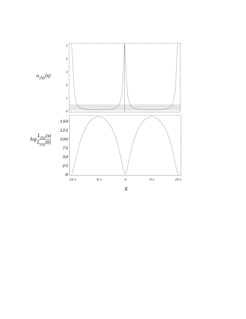
Figure 6.2: Global behavior of the superoscillatory function $\langle\gamma/2|e^{i\hat{A}\frac{x}{N}}|\!-\!\gamma/2\rangle^{N}$, in terms of the local frequency of phase oscillation $\alpha_{(N)}(x)$ and the logarithm of the likelihood factor, for $\alpha(0)=5$, $N=50$. The shaded strip indicates the region of normal oscillatory behavior.

Let us now give a general argument as to why this exponential rise about the super-oscillatory region is to be expected. Suppose one wishes to probe some arbitrary transition with an amplitude function $g(x)$ built up of modes of wave number $|k|<k_{max}$,

$$g(x)=\int_{-k_{max}}^{k_{max}}dk\,e^{ikx}\tilde{g}(k)\ ,$$ (6.20)

and which on the other hand shows super-oscillatory behavior $g(x)\simeq e^{iKx}$ about the region $-l\leq x<l$ with local wave number $K\gg k_{max}+\pi/l$. The intention is then to isolate the region by choosing an appropriate test function $\phi_{i}(x)$ suppressing the rise in magnitude away from the super-oscillatory region, so that

$$\tilde{\phi}_{f}(p)\propto\int_{-\infty}^{\infty}dx\,e^{-ipx}g(x)\ \phi_{i}(x)\simeq\tilde{\phi}_{i}(p-K)\,.$$ (6.21)

Here, we denote explicitly Fourier transforms in the $p$ representation with a tilde. Consider then the following function in the momentum representation

$$\tilde{\phi}(p)=\left\{\begin{array}[]{cc}e^{-\frac{1}{(p_{o}^{2}-p^{2})}}&|p|<p_{o}\\ 0&|p|>p_{o}\end{array}\right.\,.$$ (6.22)

This “bump” function (see Fig. 6.3) is common in analysis; its main property is that while the function is clearly not analytic, it nevertheless has derivatives of all orders for all values of $p$, including the bounds of its support $p=\pm p_{o}$.

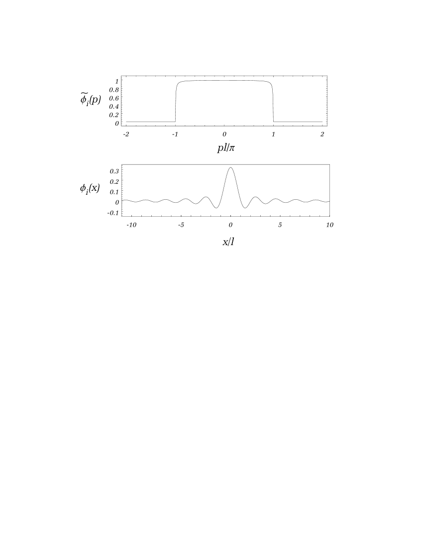
Figure 6.3: The “bump” function and its Fourier transform

Now, from the convolution theorem we know that $\tilde{\phi}_{f}(p)$ can be written exactly as

$$\tilde{\phi}_{f}(p)=\int_{-k_{max}}^{k_{max}}dk\,\tilde{g}(k)\,\tilde{\phi}(p-k)\,.$$ (6.23)

It is clear therefore that if we choose $p_{o}\simeq\pi/l$ in such a way that $k_{max}+p_{o}<K$, the support of $\tilde{\phi}_{f}(p)$ vanishes around the superoscillatory wave number $p\simeq K$ and the function is inadmissible as a probe. In turn this entails that the Fourier transform $\phi_{i}(x)$ of the “bump”, which is a function peaked at $x=0$ of width of order $l$, is nevertheless unable to suppress the rise in magnitude of $g(x)$ outside the super-oscillatory region. In other words, the rise in $g(x)$ has to be faster than the fall-off rate of $\phi_{i}(x)$. It is then easy to show that $\phi_{i}(x)$ falls-off faster at infinity than any power of $x$. For this one notes that since $\tilde{\phi}_{i}(p)$ has derivatives of all orders, then the expectation value of any power of $x$ can be written as

$$\langle x^{n}\rangle=\int dx\,x^{n}\phi_{i}(x)^{2}=\int\,dp\,\tilde{\phi}(p)\left(\frac{d}{idp}\right)^{n}\tilde{\phi}(p)$$ (6.24)

Since furthermore $\tilde{\phi}(p)$ is bounded, one then has

$$\langle x^{n}\rangle<\infty\,\ \forall n\geq 0\,.$$ (6.25)

Taking even $n=2m$, we then have for any $m\geq 0$,

$$\lim_{x\rightarrow\pm\infty}|x|^{m}\phi_{i}(x)=0\,.$$ (6.26)

We conclude that the rise in $g(x)$ away from the super-oscillating region must be of exponential order.

6.2 Illustration of Likelihood Effects in The Weak Regime

We have thus seen how anomalously long periods of super-oscillatory behavior in the phase of the amplitude function can occur in conjunction with an exponential behavior of the likelihood factor. The combination of these two anomalous behaviors provides a good illustration of two previously mentioned effects associated with the likelihood factor in the weak regime:

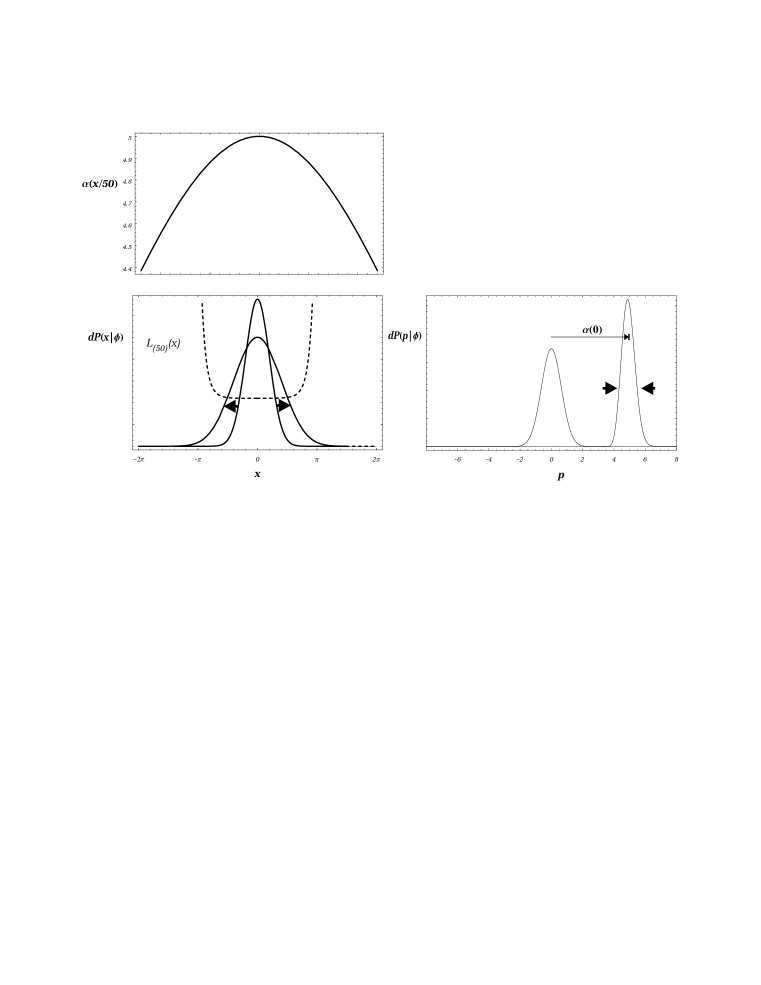
Figure 6.4: The “stretch/squeeze” effect. The dotted lines indicate the likelihood factor and the arrows the effect on the prior distribution.

The first is the “stretch/squeeze” effect. The effect is most notorious when the region is sampled precisely at the point of minimum likelihood, with the most docile exponential distribution that is still robust enough to overcome the exponential rise. In the case of the spins, the fall-off rate of the distribution is suggested by the leading order behavior to the log-likelihood factor around $x=0$, which as one can see from Eq. (6.13), is quadratic. With this suggestion, the test function $\phi_{i}(x)$ should be a Gaussian and a numerical calculation shows that indeed it does the job. We show this in Fig. 6.4 for the case of $\alpha(0)=5$, $N=50$, and an initial Gaussian of width $\sigma=\pi/4$ in $x$ . The sharp rise of the likelihood factor in both directions around $x=0$ entails a posterior distribution in $x$ that is wider by a factor of approximately

$$\frac{1}{1-2\frac{\alpha(0)^{2}\sigma^{2}}{50}}\simeq 1.6\,.$$ (6.27)

This stretch in $x$ translates to a corresponding squeeze in the distribution in $p$, which is shown shifted by the sampled weak value $\alpha(0)\simeq 5$. Note that although the posterior distribution in $x$ is wider than the prior, the dispersion in $\alpha(0)$ is still small enough for the squeeze to be evident in the pointer variable distribution. As mentioned earlier, the relative uncertainty is suppressed by an additional factor $1/\sqrt{N}$.

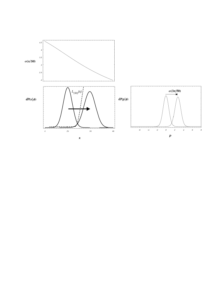
Figure 6.5: The “shift” effect. While the prior distribution in $x$ is centered around $x=2\pi$, the likelihood factor rises so fast that the posterior distribution ends up centered at $x\simeq 3\pi$. The sampled weak value The dotted lines indicate the likelihood factor and the arrows the effect on the prior dstribution.

Figure 6.6: The biased weak value $\alpha(x^{\prime}/N)$ vs. the actual weak value for different prior locations $x$ and the same uncertainty in $\sigma=\pi/4$. The jagged behavior at the peaks is due to instabilities in the root-location algorithm.

A second likelihood effect is the “shift”. The effect sets in as the location of the sampled region is moved away from the minimum likelihood point, in which case the likelihood factor overwhelmingly favors one direction in $x$. Again, if the distribution is docile enough the effect can become notorious. We illustrate this in Fig. 6.5 with the same settings as before, except that the location of the sampled point is now taken to be $x=2\pi$. In this case, the location of the posterior distribution, call it $x^{\prime}$, is given by the solution to the equation

$$\frac{(x^{\prime}-2\pi)}{(\pi/4)^{2}}=-\beta(x^{\prime})=\frac{d}{dx}\log L_{(50)}(x^{\prime})\,.$$ (6.28)

This turns out to be, numerically, $x^{\prime}\simeq 9.03$, which is close to $3\pi$. The effect is then evidenced from the pointer variable distribution in the fact that the “kick”, instead of being the weak value at $x=2\pi$, i.e., $\alpha(2\pi/50)\simeq 3.6$, turns out to be about $30\%$ smaller, the weak value at $x=3\pi$, $\alpha(2\pi/50)\simeq 2.7$. This is interpreted as a reflection of the fact that the mean rotation angle of the spins is $3\pi/50$, as opposed to $2\pi/50$, expected a priori.

Finally, we show in Fig. 6.6 the results of a numerical calculation for a situation where one “scans” the super-oscillatory region with the same initial test function but centered at different locations. For a given prior location $x$, the figure shows the “biased” weak value at the corresponding displaced location $x^{\prime}$ vs. the actual weak value at $x$. As expected, the bias is always towards regions of increasing likelihood where the weak value is smaller. This explains the “tightening” of the weak value curve.

6.3 Negative Kinetic Energies

Another interesting illustration of super-oscillatory behavior is provided by a particle initially prepared in an eigenstate of the energy and post-selected by a position measurement in a classically disallowed region. A sufficiently weak measurement of the kinetic energy operator should then yield a negative value [16]. An example that can be solved exactly is provided by a particle prepared in the ground state of a simple harmonic oscillator, with Hamiltonian:

$$\hat{H}=\frac{\hat{k}^{2}}{2m}+\frac{1}{2}m\omega^{2}\hat{q}^{2}\,.$$ (6.29)

In the ground state $|0\rangle$, $\hat{H}$ has an eigenvalue $E=\omega/2$. If the particle is post-selected in a position $q$, then the weak value of the kinetic energy operator $\hat{T}=\frac{\hat{k}^{2}}{2m}$, immediately before the post-selection, is

$$\tau(q,x)=\frac{\langle q|\hat{H}-\frac{1}{2}m\omega^{2}\hat{q}^{2}|0\rangle}{\langle q|0\rangle}\,=\frac{\omega}{2}-\frac{1}{2}m\omega^{2}q^{2}\,.$$ (6.30)

Thus, in the rare event in which $q$ happens to lie outside the region determined by the classical tuning points $|q|<1/\sqrt{m\omega}$, the weak value $\kappa$ is a negative number.

To analyze this effect, we consider the amplitude function for such measurement, which is given by

$$\sqrt{L(x)}e^{iS(x)}\propto\langle q|e^{i\hat{T}x}|0\rangle\,m.$$ (6.31)

From the point of view of the transformations generated by $\hat{T}$, we see that the amplitude may be interpreted as the diffusion of an initial wave function $\psi_{o}(q)=\langle q|0\rangle$ with diffusion constant $D=-i/2m$ though the time $x$:

$$\sqrt{L(x)}e^{iS(x)}\propto e^{-ix\frac{\partial^{2}}{\partial q^{2}}}\psi_{0}(q)$$ (6.32)

where $\psi_{o}(q)$ is the ground-state wave function of the harmonic oscillator

$$\psi_{o}(q)=\left(\frac{m\omega}{\pi}\right)^{1/4}e^{-\left(\frac{m\omega}{2}\right)q^{2}}\,.$$ (6.33)

The diffusion problem is elementary to solve for a Gaussian. Up to inessential constants, the amplitude function is given by

$$\sqrt{L(x)}\,e^{iS(x)}\propto\frac{1}{\sqrt{1-ix\omega}}\ e^{-\frac{m\omega}{2(1-ix\omega)})q^{2}}\,.$$ (6.34)

From this we may then extract the likelihood factor and the phase:

$$L(x) \propto \frac{1}{\sqrt{1+x^{2}\omega^{2}}}e^{-\frac{m\omega}{1+x^{2}\omega^{2}}q^{2}}\,$$

$$S(x) = \frac{1}{2}\arctan(x\omega)-\frac{1}{2}m\omega^{2}\left[\frac{x}{1+x^{2}\omega^{2}}\right]q^{2}m,.$$ (6.35)

and finally, from the phase, the local weak value $\tau(q,x)=S^{\prime}(x)$

$$\tau(x)=\frac{1}{1+x^{2}\omega^{2}}\left[\frac{\omega}{2}-\frac{m\omega^{2}}{2}q^{2}\right]+\frac{m\omega^{4}x^{2}}{(1+x^{2}\omega^{2})^{2}}q^{2}$$ (6.36)

We illustrate the behavior of the Likelihood factor and the weak value $\tau(x,q)$ in Figure 6.7.

Figure 6.7: Local weak and likelihood factor value for a measurement of the kinetic energy operator, with $m=\omega=1$ and the final location of the particle $q=3$.

This behavior of the local weak value may be understood in terms of two quantities, an $x$-dependent effective frequency

$$\omega(x)\equiv\frac{\omega}{1+x^{2}\omega^{2}}\,,$$ (6.37)

and a de Broglie momentum of the particle at the location and time of the post-selection

$$\kappa(x,q)\equiv\frac{\partial{S}}{\partial q}=\frac{m\omega^{2}qx}{1+x^{2}\omega^{2}}\,.$$ (6.38)

We note that this momentum is nothing more than the weak value of the momentum for the diffused state, i.e.:

$$\kappa(x,q)={\rm Re}\frac{\langle q|\hat{k}e^{i\hat{T}x}|0\rangle}{\langle q|e^{i\hat{T}x}|0\rangle}\,.$$ (6.39)

Since this momentum vanishes when $x=0$, it may be thought of as a momentum that the apparatus imparts to the particle. The local weak value may then be expressed as a “bound” term plus a “free” term: the kinetic energy weak value for a harmonic oscillator with a renormalized frequency $\omega(x)$, plus the kinetic energy of a free particle with the de Broglie momentum

$$\tau(x)=\left[\frac{\omega(x)}{2}-\frac{m\omega^{2}(x)}{2}q^{2}\right]+\frac{\kappa^{2}(x,q)}{2m}\,.$$ (6.40)

Considering then a post-selection in which $q\gg 1/\sqrt{m\omega}$, two regimes are clearly identifiable depending on the parameter $x$:

As $x\rightarrow 0$, the renormalized frequency coincides with the initial frequency and the de Broglie momentum vanishes. The behavior is therefore that of a bound particle outside the classically forbidden region, the signature of which is a negative weak value

$$\tau(q,x)\simeq-\frac{m\omega^{2}(x)}{2}q^{2}\,;$$ (6.41)

As figure 6.7 then shows, this anomalous behavior is accompanied by a considerable “dip” in the likelihood function. Clearly, if the particle is barely disturbed, then it is only a rare event in which it will be found in the classically forbidden region. As $x$ is increased away from this region, we see at around $x\simeq 1/\omega$ a quick jump in the weak value from negative to positive, while the likelihood function is still small. This may be seen as the competition between the bound and free behaviors exhibited by $\tau(q,x)$, where the bound part still contributes a negative kinetic energy, indicating that $q$ is still in a classically disallowed region, but the free part contributes just enough to overcome this barrier.

On the other hand, the exponential jump in the likelihood function indicates a transition to a free regime where it would not have been surprising to have found the particle at large values of $q$. As one can easily see, this transition occurs when $x\omega$ is of the order of $\simeq q\sqrt{m\omega}$, which is the value necessary to lower the effective binding so that $q$ lies in the classically allowed region. Beyond this, as $x\rightarrow\infty$, the renormalized frequency goes down as $1/x^{2}\omega$ and the de Broglie momentum takes the form of a kinetic momentum with $x$ playing the role of time :

$$\kappa(q,x)\rightarrow\frac{mq}{x}\,;$$ (6.42)

the particle behaves essentially as a free particle with the expected kinetic energy

$$\tau(x,q)\simeq\frac{\kappa^{2}(x,q)}{2m}\,.$$ (6.43)

6.4 A Weak to Strong “Phase Transition”

It was suggested earlier that the qualitative difference in the conditional statistics of the weak and strong regimes of measurement could possibly be an indication of two entirely different dynamical regimes in the measurement interaction, separated by a critical transition region. In exploring this possibility, we have found that a wide number of interesting phenomena of this kind can indeed be identified and interpreted with relative ease by examining the global behavior of amplitude functions which locally exhibit super-oscillations. Thus far, we have seen how by probing the anomalous region with relatively sharp test functions, the exponential rise of the likelihood factor entails relatively mild effects on the overall shape and location of the pointer-variable distribution. On the other hand, if the probe is so wide that it cannot compete with the rise in the likelihood factor, the effect of the latter is to produce “dents” in the posterior distribution in $x$, as described for instance in Chapter 4, Fig. 4.2. The appearance of dents may then interpreted as the passage to another regime in measurement strength. We shall now give a simple example in which this other regime turns out to be the “strong” regime itself, where the conditional distribution exhibits a quantized structure.

We recall from Chapter $2$ the example of initial and final states of the system are the coherent states $|\pm\!\lambda\rangle$, for instance of a simple harmonic oscillator, for which the weak value of the occupation number operator $\hat{N}$ is $-|\lambda|^{2}$. Let us then revisit this effect from within our model.

For this we compute the amplitude function:

$$\sqrt{P(-\!\lambda|x\lambda)}\,e^{iS(x)}\,=\langle-\!\lambda|e^{i\hat{N}x}|\lambda\rangle,\,.$$ (6.44)

As we have done previously, we emphasize the role of the observable as a generator of unitary transformations and of $x$ as a transformation parameter. Here $\hat{N}$ acts as a generator of rotations in the semi-classical phase-space of coherent states. Thus, we may think of $x$ as being an angle by which, for instance, the initial coherent state is rotated clockwise in this space i.e., $e^{i\hat{N}x}|\lambda\rangle=|\lambda e^{ix}\rangle$. Now, using the spectral decomposition of $\hat{N}$, we may easily compute $\langle-\lambda|e^{i\hat{N}x}|\lambda\rangle$ in closed form:

$$\langle-\lambda|e^{i\hat{N}x}|\lambda\rangle = \sum_{n=0}^{\infty}e^{-|\lambda|^{2}}\frac{(-|\lambda|^{2})^{n}}{n!}e^{inx}$$ (6.45)

$$= e^{-|\lambda|^{2}-|\lambda|^{2}e^{ix}}\,.$$

Hence, we see that the action for this rotation is

$$S(x)=-|\lambda|^{2}\sin x\,,$$ (6.46)

while the likelihood factor is

$$L(x)\propto\exp\left[-2|\lambda|^{2}\cos x\right]\,.$$ (6.47)

The reaction to the rotation is then the local weak value of $\hat{N}$, call it $\nu(x)$:

$$\nu(x)=S^{\prime}(x)=-|\lambda|^{2}\cos x\,,$$ (6.48)

and indeed we see that it takes the value $-|\lambda|^{2}$ at the point of null rotation $x=0$.

Moreover, we see for large $|\lambda|$ another example of a super-oscillating function, in this case a series of positive frequency modes, the phase of which shows a negative local frequency of oscillation $50\%$ of the time. And again the “catch”: the periods where the function shows superoscillation correspond precisely to those periods where the rotation angle $x$ is such that the two coherent states $|\!-\lambda\rangle$ and $|\lambda e^{ix}\rangle$ are opposed by an angle of more than $\pi/2$, where the overlap is minimal (Fig. 6.8).

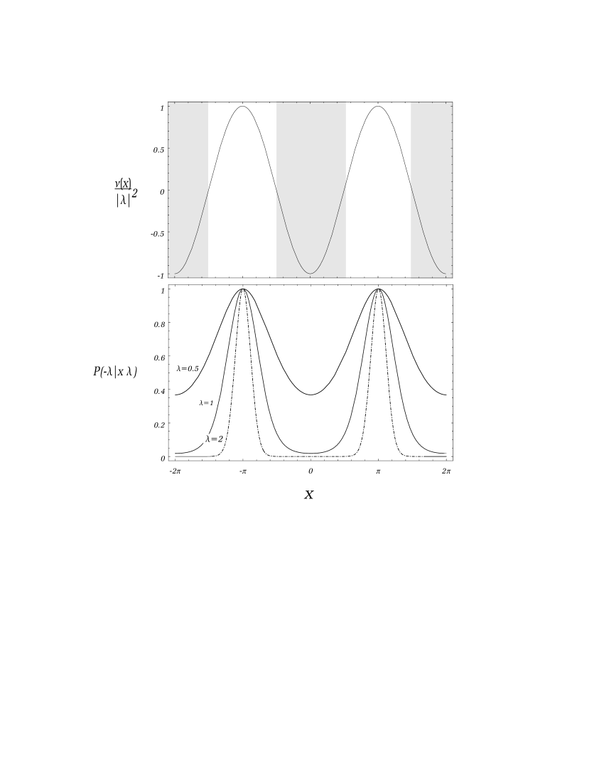
Figure 6.8: Local weak value of the occupation number operator and the respective transition probabilities for three different values of $\lambda$. The shaded regions indicate where the amplitude exhibits superoscillation

What is nice about this example is that for large values of $|\lambda|^{2}$, it provides a very simple illustration of a transition from one regime to the other depending on the width of the initial test function $\phi_{i}(x)$ (see Fig. 6.9) For this, we consider a initial minimum uncertainty preparation for $\phi_{i}(x)$ with a standard deviation $\sigma$ in $x$, centered around $x=0$. Apart from a normalization factor, the relative initial wave function, here denoted simply as $\phi_{i}^{(\lambda)}$, may then be expressed as

$$\phi_{i}^{(\lambda)}(x)=\sqrt{L(x)}\phi_{i}(x)\propto\exp\left[-|\lambda|^{2}\cos(x)-\frac{x^{2}}{4\sigma^{2}}\right]\,.$$ (6.49)

As we can see, close to $x=0$ the factor $\sqrt{L(x)}$ behaves as $\propto e^{+|\lambda|^{2}x^{2}/2}$. This means that for a weak measurement of the “impossible” value $\nu(x)=-|\lambda|^{2}$, $\phi_{i}(x)$ should fall-off fast enough to suppress this exponential rise; a weakness condition is therefore

$$\sigma\ll\frac{1}{\sqrt{2}|\lambda|}\,.$$ (6.50)

Under such conditions $\phi_{i}^{(\lambda)}$ has a single peak around $x=0$ and may be treated in a Gaussian approximation about $x=0$ if sufficiently sharp

$$\phi_{i}^{(\lambda)}(x)\simeq(2\pi\sigma_{eff}^{2})^{-1/4}e^{-\frac{x^{2}}{4\sigma_{eff}^{2}}}\,,$$ (6.51)

where the effective width is given by

$$\sigma_{eff}\simeq\frac{\sigma}{\sqrt{1-2|\lambda|^{2}\sigma^{2}}}\,.$$ (6.52)

As before, the posterior distribution in $x$ shows the characteristic stretching discussed earlier.

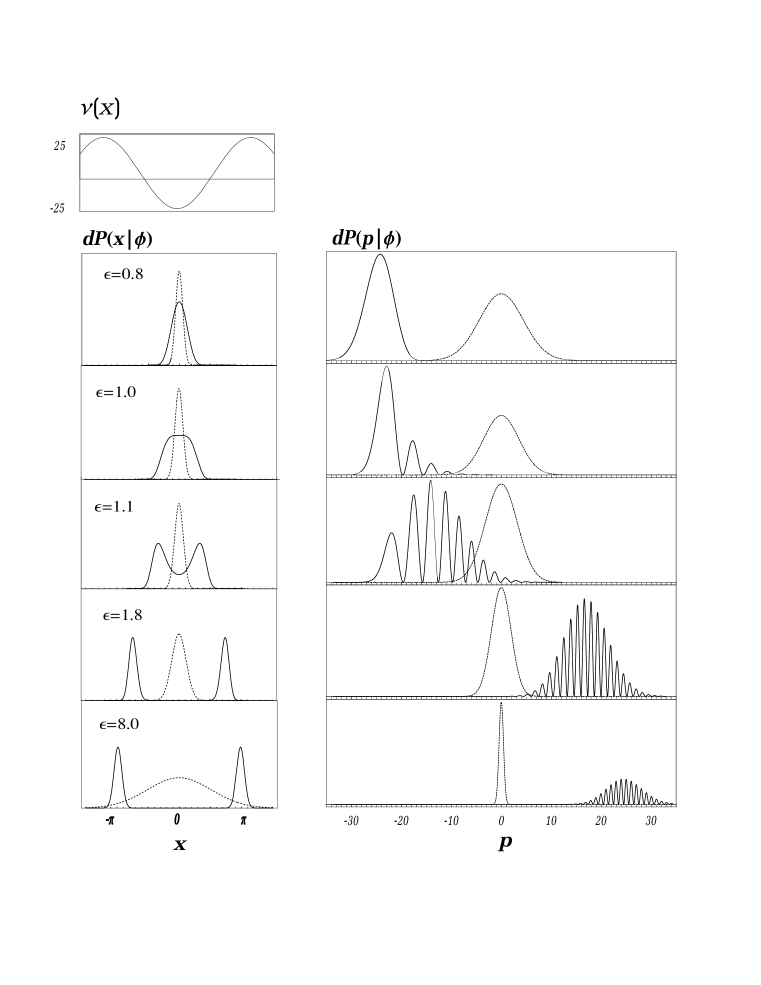
Figure 6.9: Critical behavior in passing from the weak to strong regimes, as a function of the criticality parameter $\epsilon=2\sigma^{2}|\lambda|^{2}$, with $|\lambda|^{2}=25$ (see text). The dotted lines indicate the initial distributions in both representations.

This Gaussian approximation breaks down however as $\sigma$ approaches the critical value $\sigma=1/\sqrt{2}\lambda$. If $|\lambda|^{2}$ is sufficiently large, the behavior around this critical region can be described by keeping only the quadratic and quartic terms in the exponential, in which case

$$\phi_{i}^{(\lambda)}(x)\simeq\exp\left[-\frac{1}{4\sigma^{2}}(1-2\sigma^{2}|\lambda|^{2})x^{2}-\frac{|\lambda|^{2}}{4!}x^{4}\right]\,.$$ (6.53)

Close to the critical region, one then has the characteristic behavior of a second-order phase transition: At the critical point, only the quartic terms contributes. One then has a distribution the variance of which scales as

$$\Delta x^{2}\propto\frac{\int dx\,x^{2}e^{-|\lambda|^{2}x^{4}/12}}{\int dx\,e^{-|\lambda|^{2}x^{4}/12}}\simeq|\lambda|^{-1}$$ (6.54)

Clearly, for large enough $|\lambda|$ the critical point can be reached well within the super-oscillatory region, where the average shift of the pointer is still close to $-|\lambda|^{2}$.

Now, as $\sigma$ is increased away from its critical value, the point $x=0$ becomes a local minimum and the distribution acquires two peaks. Defining a criticality parameter

$$\epsilon\equiv 2\sigma^{2}|\lambda|^{2}\,,$$ (6.55)

the two peaks are given close to the critical pont $\epsilon=1$ at:

$$\tilde{x}\simeq\pm\sqrt{6\left(\frac{\epsilon-1}{\epsilon}\right)}\,.$$ (6.56)

If one performs a Gaussian approximation about each peak, the resultant variance there goes as

$$\Delta x\simeq\frac{1}{|\lambda|}\sqrt{\frac{\epsilon}{(\epsilon-1)}}\,$$ (6.57)

One should then expect the distribution to break up into two well-separated distributions when $\Delta x\leq\tilde{x}$, which implies that

$$\left(\frac{(\epsilon-1)}{\epsilon}\right)\geq\frac{\sqrt{6}}{|\lambda|}\,.$$ (6.58)

For large $|\lambda|$ this again entails that the separation occurs for very moderate deviations of $\sigma$ about its critical value in which case the two peaks still lie within the super-oscillatory region.

As $\sigma$ is further increased away from this critical region, the two peaks rapidly separate due to the exponential increase in the likelihood factor towards the regions of overwhelming likelihood $x=\pm\pi$, where say the initial state $|\lambda\rangle$ is rotated to $|-\lambda\rangle$. Again, for large $|\lambda|$ each peak may be treated in the Gaussian approximation, where the location $\tilde{x}$ of each is given by the first non-vanishing solutions to the equation

$$\tilde{x}=\epsilon\sin(\tilde{x})\,.$$ (6.59)

The positive roots of this equation are shown in Fig. 6.10 as a function of $\epsilon$.

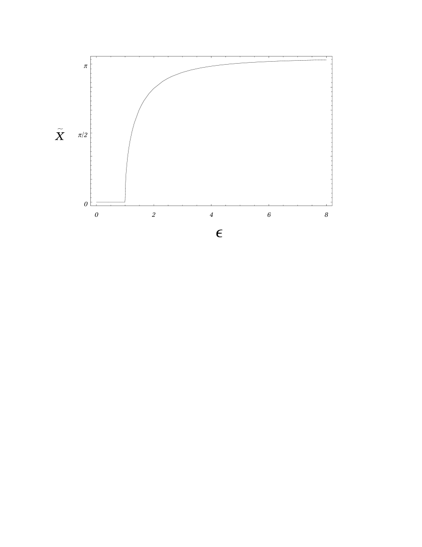
Figure 6.10: Positive solutions for the location of the peaks as a function of the critical parameter $\epsilon$.

Up to normalization, $\phi_{i}^{(\lambda)}(x)$ may then be written as

$$\phi_{i}^{(\lambda)}(x)\propto e^{-\frac{(x-\tilde{x})^{2}}{4\sigma_{eff}^{2}}}+e^{-\frac{(x+\tilde{x})^{2}}{4\sigma_{eff}^{2}}}\,,$$ (6.60)

with an effective width $\sigma_{eff}$. For the effective width, we note that since the weak value $\nu(x)$ is symmetric about the origin, and the second logarithmic derivative of $\phi_{i}^{(\lambda)}(x)$ evaluated at the peak $\tilde{x}$ is

$$-\frac{1}{2\sigma^{2}}+|\lambda|^{2}\cos(\tilde{x})=-\frac{1}{2\sigma^{2}}-\nu(\tilde{x})\,,$$ (6.61)

the width can be expressed in terms of the local weak value at $\tilde{x}$ as

$$\sigma_{eff}=\frac{\sigma}{\sqrt{1+2\sigma^{2}\nu(\tilde{x})}}\,.$$ (6.62)

Now, as each peak samples the same weak value,the average kick of the pointer variable is given approximately by

$$\langle p_{f}\rangle=\nu(\tilde{x})\simeq-|\lambda|^{2}\cos(\tilde{x})\,.$$ (6.63)

We can then see that as sigma is increased, the kick goes from $-|\lambda|^{2}$ in the super-oscillatory region to the weak value at the regions $\tilde{x}=\pm\pi$ of maximum likelihood, $\nu(\pm\pi)=+|\lambda|^{2}$.

However, once the peaks are separated in $x$-space, the resultant distribution in $p$ exhibits interference fringes. Each peak contributes in the relative wave function for $p$ a phase factor $e^{\pm ip|\tilde{x}|\pm iS(|\tilde{x}|)}$ corresponding to its location in $x$, i.e.,

$$\phi_{f}^{(\lambda)}(p) \propto \int_{-\infty}^{\infty}dx\,e^{-ipx+iS(x)}\phi_{i}^{(\lambda)}(x)$$ (6.64)

$$\simeq 2\cos(p\tilde{x}-S(\tilde{x}))\,\int_{-\infty}^{\infty}d\xi\,e^{-ip\xi+i\nu(\tilde{x})\xi}e^{-\frac{\xi^{2}}{4\sigma_{eff}^{2}}}\,,$$

where we have used the fact that $S(x)$ is odd and $\nu(x)$ is even. Using the defining equations for $\tilde{x}$ and $\epsilon$, the final pointer variable distribution takes the form of a Gaussian packet, of width $1/2\sigma_{eff}$, times a modulation factor coming from the interference between the two peaks:

$$dP(p|\phi_{f}^{(\lambda)})\propto\exp\left[-\frac{1}{2\Delta p_{f}^{2}}\left(p-\nu(\tilde{x})\right)^{2}\right]\ \cos^{2}\left[\left(p+\frac{|\lambda|^{2}}{\epsilon}\right)\tilde{x}\right]\,,$$ (6.65)

where

$$\Delta p_{f}^{2}=\Delta p_{i}^{2}+\frac{1}{2}\nu(\tilde{x})\,$$ (6.66)

and $\Delta p_{i}=\frac{1}{2\sigma}$. As one can then see, when the criticality parameter $\epsilon$ becomes large, $\tilde{x}\rightarrow\pi$, and around the region $p\simeq|\lambda|^{2}$ the modulation factor becomes a maximum at integer values of $p$ and zero at half integer values. One thus obtains a distribution in $p$, centered at the weak value $p=+|\lambda|^{2}$, of variance $\Delta p_{f}^{2}=\Delta p_{i}^{2}+|\lambda|^{2}/2$, and which reflects the positive spectrum of the occupation number operator.

The beautiful thing is that in this way arrive at an alternative description of the emergent quantized structure in the conditional distribution of the data. According to the the non-linear model, the initially sharp wave function in $p$ corresponds to a wide function in $x$ in which the tails brush two regions of maximum likelihood $\tilde{x}=\pm\pi$. Each region corresponds to a possible rotation of the initial state to the final state, where the signs denote the sense of rotation. While the a priori probability of either rotation is quite small, the fact that the final state was indeed $|-\lambda\rangle$ entails an enormous probability that in fact the initial state was rotated. This is then reflected in the two narrow peaks at $x=\pm\pi$, and the fact that the shift is the weak value $|\lambda|^{2}=\langle-\lambda|\hat{N}|-\lambda\rangle$, corresponding to the same initial and final states. What is then seen in terms of the standard linear model as a superposition of shifts of the initial narrow packet in $p$, with an envelope given by the spectral amplitudes, in the non-linear model is the wide distribution corresponding to a weak measurement at the rotated configuration of the system, but modulated by an interference pattern generated by two different phases acquired along the two possible senses of rotation. It is also interesting to note that close to the critical region ($\epsilon=1.1$), one also obtains from the interference of the two peaks, a sort of quantization in which the “eigenvalues” now fall on non-integer negative numbers.

6.5 Overall Distribution of Weak Values

The “pearls” we have dealt with in the above examples are admittedly quite rare. Given a particular post-selection, the probability of finding them is exponentially small. Even then, one must be extremely careful in the preparation of the apparatus so that indeed one samples those exponentially suppressed regions. One may wonder therefore as to how unlikely are “eccentric” weak values overall?

To answer this question, let us consider the probability distribution of weak values when only an initial condition $|\psi\rangle$ is given and no additional information is known about the final state. So far, we have dealt with fixed final bases, i.e., $B=\{|\psi_{\mu}\rangle\}$. Information about the basis is already relevant information as it singles out only a handful of all possible pairs of initial and final states are selected. The distribution is then given by

$$dP(\alpha|\psi B)=\sum_{|\psi_{\mu}\rangle\in B}\|\langle\psi_{\mu}|\psi\rangle\|^{2}\delta\left(\alpha-{\rm Re}\frac{\langle\psi_{\mu}|\hat{A}|\psi\rangle}{\langle\psi_{\mu}|\psi\rangle}\right)\,.$$ (6.67)

As we have seen earlier, the average $\overline{\alpha}$ of the distribution is the expectation value of $\hat{A}$ given $\psi\rangle$, $\langle\hat{A}\rangle$, and is thus basis-independent. On the other hand, the remaining information contained in this distribution, i.e. the scatter about its average is basis-dependent.

To obtain a basis-independent expression, we should then consider all possible final states that may occur under all possible post-selections that one may envision, giving prior probabilities to each final state. In this case, the weight factor which is naturally defined is the Hilbert-space overlap between the initial and final states. Thus one has

$$dP(\alpha|\psi)=\frac{\int D_{|\psi_{\mu}\rangle}\,\|\langle\psi_{\mu}|\psi\rangle\|^{2}\delta\left(\alpha-{\rm Re}\frac{\langle\psi_{\mu}|\hat{A}|\psi\rangle}{\langle\psi_{\mu}|\psi\rangle}\right)}{\int D_{|\psi_{\mu}\rangle}\,\|\langle\psi_{\mu}|\psi\rangle\|^{2}}\,.$$ (6.68)

where $D_{|\psi_{\mu}\rangle}$ is a uniform measure over all states $|\psi_{\mu}\rangle$ in Hilbert space. Note that in fact the integral overcounts each final state since two states differing only by a phase factor are equivalent; this overlap is taken care of by the normalization factor in the denominator. To calculate this integral, it becomes more convenient however to express it as a marginal distribution of the overall distribution $d^{2}P(\alpha\beta|\psi)=d^{2}P(z|\psi)$ for

$$z=\alpha+i\beta=\frac{\langle\psi_{\mu}|\hat{A}|\psi\rangle}{\langle\psi_{\mu}|\psi\rangle}\,,$$ (6.69)

both the real and imaginary parts of the complex weak value:

$$dP(\alpha|\psi)=\int_{\beta}d^{2}P(\alpha\beta|\psi)$$ (6.70)

The two-dimensional probability distribution for $z$ is then given by

$$d^{2}P(z|\psi)=d^{2}z\frac{\int D_{|\psi_{\mu}\rangle}\,\|\langle\psi_{\mu}|\psi\rangle\|^{2}\delta^{2}\left(z-\frac{\langle\psi_{\mu}|\hat{A}|\psi_{1}\rangle}{\langle\psi_{\mu}|\psi\rangle}\right)}{\int D_{|\psi_{\mu}\rangle}\,\|\langle\psi_{\mu}|\psi\rangle\|^{2}}\,,$$ (6.71)

where $d^{2}z=d\alpha d\beta$ and the complex delta function for a complex number $z=x+iy$ is defined as

$$\delta^{2}(z-z_{o})\equiv\delta(x-x_{o})\,\delta(y-y_{o})\,.$$ (6.72)

The integral (6.71) is easily evaluated if one notes a simple trick [5] that yields an optimal parametrization of the final state: for any hermitian operator $\hat{A}$, its action on a quantum state $|\psi\rangle$ can be written as

$$\hat{A}|\psi\rangle=\langle\hat{A}\rangle|\psi\rangle+\Delta A|\psi_{\perp}\rangle$$ (6.73)

where $\langle\hat{A}\rangle$ is the standard expectation value $\langle\psi|\hat{A}|\psi\rangle$, the vector $|\psi_{\perp}\rangle$ is a certain state orthogonal to $|\psi\rangle$, and $\Delta A$ is the standard uncertainty

$$\Delta A=\sqrt{\,\langle\psi|\left(\hat{A}-\langle\hat{A}\rangle\right)^{2}|\psi\rangle}\,.$$ (6.74)

This allows us then to select a frame of mutually orthogonal vectors comprised of $|\psi\rangle$, $|\psi_{\perp}\rangle$ and some other number of vectors $|i\rangle$, $N-2$ of them if $N$ is the dimensionality of the Hilbert space. One may then expand $|\psi_{\mu}\rangle$ in that frame as

$$|\psi_{\mu}\rangle=w_{1}|\psi\rangle+w_{2}|\psi_{\perp}\rangle+\sum_{i=3}^{N}w_{i}|i\rangle$$ (6.75)

where the complex coefficients $\{w_{i}\}$ are bound by the constraint

$$1=\sum_{i=1}{N}\|w_{i}\|^{2}$$ (6.76)

With this parametrization, the integral (6.71) becomes the complex integral

$$d^{2}P(z|\psi)=d^{2}z\frac{\int\,\prod_{i=1}^{N}\,d^{2}w_{i}\,\delta\left(1-\sum_{i=1}^{N}\|w_{i}\|^{2}\right)\|w_{1}\|^{2}\delta^{2}\left(z-\langle A\rangle-\Delta A\frac{w_{2}}{w_{1}}\right)}{\int\,\prod_{i=1}^{N}\,\delta\left(1-\sum_{i=1}^{N}\|w_{i}\|^{2}\right)\|w_{1}\|^{2}}\,.$$ (6.77)

We now note a useful property for the $2$-d complex delta function:

$$\delta^{2}(wz-wz_{o})=\frac{1}{\|w\|^{2}}\delta^{2}(z-z_{o})\,,$$ (6.78)

in terms of which one obtains:

$$d^{2}P(z|\psi)=d^{2}z\frac{\int\,\prod_{i=1}^{N}\,d^{2}w_{i}\,\delta\left(1-\sum_{i=1}^{N}\|w_{i}\|^{2}\right)\|w_{1}\|^{4}\delta^{2}\left(w_{2}-w_{1}\frac{z-\langle A\rangle}{\Delta A}\right)}{\int\,\prod_{i=1}^{N}\,\delta\left(1-\sum_{i=1}^{N}\|w_{i}\|^{2}\right)\|w_{1}\|^{2}}\,.$$ (6.79)

The rightmost delta function fixes the value of $w_{2}$ as a function of $w_{1}$, and hence integrating over $w_{2}$ we have for the constraint delta-function:

$$\delta\left(1-\sum_{i=1}^{N}\|w_{i}\|^{2}\right)\rightarrow\delta\left[1-\left(1+\left\|\frac{z-\langle A\rangle}{\Delta A}\right\|^{2}\right)\|w_{1}\|^{2}+\sum_{i=3}^{N}\|w_{i}\|^{2}\right]\,.$$ (6.80)

Performing the change of variables

$$w_{1}\rightarrow\sqrt{1+\left\|\frac{z-\langle A\rangle}{\Delta A}\right\|^{2}}\ w_{1}$$ (6.81)

in the upper integral, one obtains:

$$d^{2}P(z|\psi)=K\frac{\ d^{2}z}{\Delta A^{2}}\ \frac{1}{\left[\ 1+\left\|\frac{z-\langle A\rangle}{\Delta A}\right\|^{2}\ \right]^{3}}\$$ (6.82)

where the normalization constant is

$$K=\frac{\int\prod_{i=1}^{N-1}\,d^{2}w_{i}\,\delta\left(1-\sum_{i=1}^{N-1}\|w_{i}\|^{2}\right)\|w_{1}\|^{4}}{\int\,\prod_{i=1}^{N}\,d^{2}w_{i}\,\delta\left(1-\sum_{i=1}^{N}\|w_{i}\|^{2}\right)\|w_{1}\|^{2}}\,.$$ (6.83)

Finally, computing this constant instead by imposing the normalization condition

$$K^{-1}=\int\frac{d^{2}r}{[\,1+r^{2}\,]^{3}}=\frac{\pi}{2}\,.$$ (6.84)

we obtain for the $2$-dimensional distribution

$$d^{2}P(\alpha\beta|\psi)=\frac{2}{\pi}\frac{d\alpha d\beta}{\Delta A^{2}}\ \frac{1}{\left[\ 1+\left(\frac{\alpha-\langle A\rangle}{\Delta A}\right)^{2}+\left(\frac{\beta}{\Delta A}\right)^{2}\ \right]^{3}}\,.$$ (6.85)

The distribution then shows that the complex weak value of $\hat{A}$ is symmetrically distributed about $z=\langle a\rangle$, with a width of order $\Delta A$.

Concentrating finally on the real part, we find after integrating over $\beta$ the marginal distribution

$$dP(\alpha|\psi)=\frac{3}{4}\frac{d\alpha}{\Delta A}\frac{1}{\left[1+\left(\frac{\alpha-\langle A\rangle}{\Delta A}\right)^{2}\right]^{5/2}}\,,$$ (6.86)

which is shown in Fig. (6.11)  .

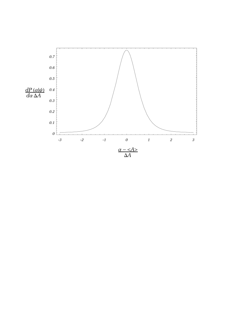
Figure 6.11: Overall probability distribution function for the weak value $\alpha$ of $\hat{A}$ given an initial state $|\psi\rangle$.

The distribution admits two non-trivial central moments, the mean and variance, which are easily computed:

$$\overline{\alpha} = \langle\hat{A}\rangle$$

$$\overline{\Delta\alpha} = \frac{\Delta A}{\sqrt{2}}\,.$$ (6.87)

Again we note that while for any observable $\hat{A}$ the overall distribution of weak values extends all the way to infinity (unless, of course, $|\psi\rangle$ is an eigenstate of $\hat{A}$), the concentration of weak values is nevertheless tighter about the mean than the concentration of eigenvalues given the spectral distribution $\langle\psi|\hat{\Pi}_{a}|\psi\rangle$.

To answer then the question posed at the beginning of the section as to how unlikely are eccentric weak values, let us consider as a representative example an operator $\hat{A}$, the spectrum of which is bounded by $\pm a_{max}$, and a state $|\psi\rangle$ yielding a uniform distribution of eigenvalues within this interval. In such case $\langle\hat{A}\rangle=0$ and $\Delta A=a_{max}/\sqrt{3}$; the probability of a weak value outside the spectrum is therefore

$$P(|\alpha|>a_{max}|\psi)=1-\frac{3}{4}\int_{-\sqrt{3}}^{\sqrt{3}}\frac{dx}{\left[1+x^{2}\right]^{5/2}}\simeq 0.026\,.$$ (6.88)

It is interesting to note therefore that when all possible final states are taken into account, the relative proportion of eccentric weak values is of the order of one in a hundred, clearly not an extraordinarily small number.

Chapter 7 Conclusion and Open Questions

The model presented in this dissertation may be regarded as a modest step in a more ambitious program suggested by the Two-Vector Formulation, namely, the construction of a general theory of measurement in quantum mechanics based entirely on time-symmetric ensembles and weak values. It may be worthwhile then to give a brief account of what has been achieved here as well as to point out several questions that remain open for future exploration in this direction.

As a preliminary motivation for the non-linear model, we have suggested a sort of complementarity between two “ideal” measurement situations, the standard or strong measurement scheme and the weak measurement scheme, each of which corresponds to the initial conditions of the measuring apparatus being controlled for either optimal precision or conversely, for minimal disturbance of the measured system. A clear distinction between the two extremes becomes evident when the statistics are analyzed against fixed initial and final conditions on the system: in one extreme, the statistics exhibit a spectral distribution for the measured observable, whereas in the other the apparatus appears to show a response to a definite weak value. By identifying these two extremes, the intermediate “limbo” region of non-ideal measurements becomes of considerable interest as one may expect that the transition form one description to the other is accompanied by a qualitative change in the physics of the measurement interaction.

As a way of bridging the two descriptions, we have suggested with the non-linear model an alternative picture based on weak values for general non-ideal von Neumann-type measurements. In this description, the apparatus is seen as driving the system, via-back reaction, into various “configurations”–i.e., pairs of initial and final states, parameterized by what we have termed the reaction variable of the apparatus. Each configuration determines a local weak value for the measured observable as well as a weight factor, the likelihood factor. The non-linear model may thus be viewed as the “quantized” version of a picture which in fact proves to have a direct classical correspondence: the possible configurations of the system are “sampled” with a probability distribution for the reaction variable determined by the likelihood factor, and from each configuration the pointer variable receives a corresponding “kick” proportional to the local weak value. While direct quantitative agreement with the classical picture of statistical sampling is attained only in the expectation value of the pointer variable, the picture of sampling nevertheless proves useful in analyzing the response of the apparatus at the level of wave functions, where the resulting quantum state of the apparatus can be decomposed as a superposition of weak measurements. The non-linear model therefore provides a complement to the more standard analysis based on the spectral decomposition of the measured observable.

The underlying motivation for this dual description is, as mentioned in the introduction, to gain a further understanding of the physics of the measurement interaction. The “phase-transition” at the end of Chapter $6$ gives a particularly good example of a situation in which one may benefit from this dual description, as it is from the point of view of the reaction variable where one sees a qualitative change in the physics of the interaction as one crosses from the weak to strong regimes at a definite critical measurement strength. Such transitions should in fact be quite generic as one only needs to identify situations where the likelihood factor exhibits a drastic “dip” such as for instance around regions of anomalous superoscillatory behavior. It should be interesting therefore to characterize the degree of universality in these transitions.

It would also be desirable to further explore how the standard ideal measurement scheme relates to the picture of sampling weak values. In Chapter $3$ and the “phase-transition” example in Chapter $6$ we have already given two examples where the emergence of a quantized structure in the resulting distribution of the data is viewed, from the sampling picture, as an interference phenomenon in the quantum-mechanical response of the apparatus to a non-linear effective action. From the point of view of the non-linear model therefore, quantization appears to be more of an emergent property of the whole measurement interaction as opposed to an intrinsic property of the system in isolation.

It may then be worthwhile to pursue this idea further in systems, such as a spin-$1/2$, considered to be “intrinsically” quantized. In particular, we recall how in the case of orbital angular momentum described in Chapter $3$, a local sampling of the weak value reveals the classical angular momentum, whereas integer value quantization emerges only from a global sampling in a manner akin to the appearance of band-structures under periodic potentials. Could it then not be the case that in a similar fashion, underlying the two “bands” in a Stern-Gerlach measurement of Spin-$1/2$ is in fact a continuous angular momentum vector, such as for instance the one defined by the weak values of the three spin components (Fig. 1.3)? The non-linear model already suggests how this apparently contradictory picture can be reconciled with quantization: the quantized structure of the apparatus wave function coming from the periodicity in the sampling in addition to a likelihood factor which effectively suppresses unusually high values of angular momentum outside of the usual range $[-1/2,1/2]$. The idea is certainly interesting and novel enough to warrant further investigation.

In this respect, another aspect worth exploring is the “configuration” space of the system that is sampled in the measurement process according to the Two-Vector description. In the original formulation [5, 6, 7], both the real and imaginary parts of the complex weak value are viewed as being equally fundamental elements of the physical property associated with the measured observable. To specify univocally the complex weak values for all elements of the observable algebra, one therefore needs to assign an ordered pair of state vectors, as the imaginary part of $\frac{\langle\psi_{2}|\hat{A}|\psi_{1}\rangle}{\langle\psi_{2}|\psi_{1}\rangle}$ is odd under a time reversal of the boundary conditions. In the present dissertation, however, we have shown that it is only the real part of the weak value which has a straightforward interpretation in terms of mechanical effects as it can be related directly to a unitary transformation. Furthermore, we have traded the local description provided by the imaginary part for the more natural global description in terms of probability re-assessment provided by the likelihood factor. It is therefore tempting to consider a point in the “configuration” space as being defined in terms of a minimal object from which both the likelihood factor and the real weak values can be obtained. A candidate for this object is for instance the hermitian operator

$$\hat{\Omega}\equiv\frac{1}{2}\left[\frac{|\psi_{1}\rangle\langle\psi_{2}|}{\langle\psi_{2}|\psi_{1}\rangle}+\frac{|\psi_{2}\rangle\langle\psi_{1}|}{\langle\psi_{1}|\psi_{2}\rangle}\right]\,,$$ (7.1)

in terms of which, the weak value of a given observable $\hat{A}$ is $\alpha={\rm Tr}[\hat{A}\hat{\Omega}]\,$ and the weight factor $|\langle\psi_{2}|\psi_{1}\rangle|^{2}$ associated with a given pair of vectors is $(2{\rm Tr}[\hat{\Omega}^{2}]-1)^{-1}\,.$ Besides the obvious time reversal symmetry $|\psi_{1}\rangle\leftrightarrow|\psi_{2}\rangle$, a given $\hat{\Omega}$ defines a whole equivalence class of pairs connected by a non-trivial continuous $U(1)\times U(1)$ transformation. It may therefore be worthwhile to investigate the significance of this degeneracy as well as the geometry of the configuration space defined by such objects.

Another related point that needs to be pursued with greater care has to do with the single measurement event. So far, we have tried to establish a connection between the overall statistical distribution of the pointer variable and an underlying distribution of sampled weak values. Suppose however we are dealing with a single reading of the pointer variable. What can we then infer about the weak values? This seems to be a rather subtle question as the weak value distribution and the pointer distribution are ultimately related in the same way that that the probability distributions for two canonically conjugate variables are related, that is, at the level of wave functions through a Fourier transform. The idea of applying Bayes’ theorem to obtain a posterior distribution of weak values is therefore hindered to the same extent that we cannot obtain a positive-definite joint probability distribution for two canonically conjugate variables.

A way of working around this situation may be to trace the weak value in question but now on the system-apparatus composite, as the apparatus reading completes the necessary information for a two-vector description of the composite system. This however brings additional difficulties. Intuitively, one should expect that if the measurement interaction is sufficiently weak, the information provided by a single reading should not significantly modify the free history of weak values of the system. On the other hand, one need not expect this to be the case when dealing with strong measurements as a single reading already entails a re-assessment of the two-vector pair of the same extent to which in the standard formulation it entails a “collapse” of the wave function. Such problems demand a more careful examination and may be indicative of the type of difficulties that lie ahead in attempting a more rigorous ontological interpretation of the measuring process in terms of weak values.

Vita

Alonso Botero was born in Medellín, Colombia, on January 18, 1967, the son of Hernando Botero and Constanza Mejía. After completing his high school education at The Columbus School, Medellín, Colombia, in 1984, he served a year of military service. In 1986 he entered The Universidad de los Andes, Bogotá, Colombia, where he received an undergraduate degree in Physics in 1991. He obtained the degree of Master of Arts at Boston University in 1994, where he was also awarded the Goldhaber Prize for outstanding first-year student. In 1994 he entered the Graduate School at The University of Texas.

Permanent Address: Calle 11B No. 36B-53 Apt. 301, Medell n, Colombia

This dissertation was typeset with LaTeX 2ε by the author.

Bibliography

- [1] B. d’Espagnat.Veiled Reality. (Addison-Wesley, Reading, 1995)
- [2] N. Bohr. Phys. Rev. 48, 696 (1935).
- [3] Y.Aharonov, P. Bergmann, and J. Lebowitz. Phys. Rev. 134B, 1410 (1964).
- [4] W. Unruh. Ann. N.Y. Acad. Sci. 755, 560 (1995).
- [5] Y. Aharonov and L. Vaidman. Phys. Rev. A 41, 12 (1990).
- [6] Y. Aharonov and L. Vaidman. J. Phys. A 24, 2315 (1991).
- [7] Y. Aharonov and B. Reznik, Phys. Rev. A 52, 2538 (1995).
- [8] Y.Aharonov, D. Albert, A. Casher and L. Vaidman, Phys. Lett. A 124, 199 (1987).
- [9] Y.Aharonov, D. Albert, and L. Vaidman. Phys. Rev. Lett 60, 1351 (1988).
- [10] I. Duck, P. Stevenson, and E. Sudarshan. Phys. Rev. D 40, 2112 (1989).
- [11] N. Ritchie, J. Story and R. Hulet, Phys. Rev. Lett. 66, 1107 (1991).
- [12] W. Mückenheim. Physics Reports 133, 337 (1986), and references therein.
- [13] ”Inverse Problems”, D. Mc Laughlin, ed. - SIAM-AMS Proceedings. 14 (1984)
- [14] L. Vaidman. Phys. Rev. Lett. 70, 3369 (1993); L. Vaidman, Elements of Reality and the Failure of the Product Rule, Symposium on the Foundation of Modern Physics, Cologne, 1993, P.J. Lahti, P. Bush, and P. Mittelstaedt (eds.), (World Scientific, Singapore, 1993)
- [15] A.M. Steinberg. Phys. Rev. A 52, 32 (1995).
- [16] Y. Aharonov and D. Rohrlich, in Quantum Coherence, J. Anandan, ed. World Scientific, 221 (1990);
- [17] G. Iannaconne, Talk given at the Adriatico Research Conference on ”Tunnelling and its implications”, 30 July–2 August 1996, ICTP, Trieste, (quant-phys/9611018);
- [18] J. von Neumann. Mathematical Foundations of Quantum Mechanics. (Princeton University Press, Princeton, 1983)
- [19] V. B. Braginsky and F. Y. Khalili Quantum Measurement (Cambridge University Press, Cambridge,1992)
- [20] R.T. Cox. The Algebra of Probable Inference. (Johns-Hopkins Press, Baltimore, 1961).
- [21] E.T. Jaynes: Papers on Probability, Statistics and Statistical Physics. R. Rosenkrantz, ed. (Reidel, Dordrecht, 1982); E. Jaynes. Probability: The Logic of Science. In preparation. Preliminary versions available electronically at ftp://bayes.wustl.edu.
- [22] J. Bernardo and A. Smith, Bayesian Theory (Wiley, Chichester, 1994)
- [23] V. Arnold. Mathematical Methods of Classical Mechanics 2nd. ed. (Springer Verlag, Berlin, 1989)
- [24] C. DeWitt-Morette, A. Maheshwari and B. Nelson, Path Integration in Non-Relativistic Quantum Mechanics Phys. Rep. 50, 257 (1979)
- [25] I am grateful to Benni Reznik for pointing this out.
- [26] Y. Aharonov, J. Anandan, S. Popescu and L. Vaidman, Phys. Rev. Lett.64 (1990)
- [27] M. Berry. “Faster Than Fourier”. In Quantum Coherence and Reality: in celebration of the 60th birthday of Yakir Aharonov. J.S. Anandan, J. L. Safko, eds. (Wordls Scientific, Singapore,1994).
Vita