Experimental requirements for Grover’s algorithm in optical quantum computation

Abstract

The field of linear optical quantum computation (LOQC) will soon need a repertoire of experimental milestones. We make progress in this direction by describing several experiments based on Grover’s algorithm. These experiments range from a relatively simple implementation using only a single non-scalable cnot gate to the most complex, requiring two concatenated scalable cnot gates, and thus form a useful set of early milestones for LOQC. We also give a complete description of basic LOQC using polarization-encoded qubits, making use of many simplifications to the original scheme of Knill, Laflamme, and Milburn Knill et al. (2001a).

I Introduction

In the next few years, we can expect to see demonstrations of basic quantum gates in several implementations of quantum computation. With this in sight, it is natural to look ahead to what interesting quantum circuits can be built out of a small number of one- and two-qubit gates acting on a few qubits, as these circuits will provide milestones on the way to full-scale quantum computation QIS (2002).

Grover’s search algorithm Grover (1996, 1997) is a good candidate for such a milestone. It is a quantum algorithm identifying one of $N$ elements, marked by an oracle, with order $\sqrt{N}$ uses of the oracle. When the search space consists of 4 elements, the algorithm is guaranteed to produce the marked element after one use of the oracle, compared to the 2.25 uses expected in a classical search. We will see that it can be implemented using only 7 one-qubit gates and 2 two-qubit gates, which makes it an excellent target once one- and two-qubit gates have been mastered. Not surprisingly, it was one of the first algorithms to be experimentally implemented in nuclear magnetic resonance quantum computing (Chuang, Gershenfeld, and Kubinec Chuang et al. (1998) and Jones, Mosca, and Hansen Jones et al. (1998)).

A promising quantum computing technology is the linear optical quantum computation (LOQC) scheme of Knill, Laflamme, and Milburn Knill et al. (2001a) (see Gottesman, Kitaev, and Preskill Gottesman et al. (2001) for an alternative approach). In this scheme, one-qubit gates are relatively straightforward. While implementing a scalable universal two-qubit gate such as a cnot remains a challenge, such a gate is likely to be demonstrated in the next couple of years. Already, a non-scalable cnot has been approximately implemented by Pittman et al. Pittman et al. (2003). For these reasons, it is important to establish some specific LOQC milestones on the path toward building a large quantum computer, in the form of some simple algorithms on a few qubits.

This pursuit is dogged by conceptual difficulties associated with quantum algorithms on a very small number of qubits, summed up in the question: What is the criterion for “quantumness”? A reasonable criterion, particularly in the context of Grover’s algorithm, is to require a “speed-up” over the best classical algorithm. However, this notion can be hard to make sense of when the number of steps is on the order of ten, rather than millions, and the problem can easily be done by hand (not to mention by a GHz classical processor). Furthermore, sometimes the reduction in the number of steps can be achieved in an implementation whose physical requirements grow exponentially with the number of qubits, trading off time for space. The question of whether or not this counts as “quantum” has received much attention (see, for example, Kwiat et al. Kwiat et al. (2000), Bhattacharya, van den Heuvell, and Spreeuw Bhattacharya et al. (2002)).

Perhaps the best solution to this problem is a pragmatic one. In the quest to build a quantum computer large enough to provide a genuine advantage over classical computers, two things must be achieved. First, a fine level of quantum control must be demonstrated for both single qubits and pairs of qubits. Second, it will be necessary to show that the number of components (qubits and gates) in a circuit can be increased without insurmountable increases in difficulty. In particular, we must avoid exponential increases in the amount of resource usage (either time or space) — the implementation must be scalable.

Therefore, the importance of an experimental achievement of an early milestone (such as the four-element Grover’s algorithm) should be measured primarily on these criteria. A demonstration that Grover’s algorithm finds the marked item in fewer steps than is possible with a classical computer is an important goal, but it is less important than the fine level of quantum control that it implies. At this early stage of development of quantum computers, any such demonstration is a significant achievement, while a demonstration of such control in a scalable manner is likely to be significantly more difficult and consequently more impressive.

This is illustrated by the experiment of Kwiat et al. Kwiat et al. (2000), which demonstrated the ability to implement the search algorithm in a quantum optical system, but using an encoding that is not scalable — as they point out, the number of optical elements that they require grows exponentially in the number of qubits in their system. Thus, although their techniques might be successfully extended to a few qubits, they are not practical as the basis for an approach to building a quantum computer.

In contrast, we are explicitly concerned with developing experimental milestones on the path toward full-scale quantum computation in optical systems. We show that Grover’s algorithm on four elements provides several experiments that gradually increase in complexity. The simplest version requires little more than a single, coincidence-basis cnot gate together with a source of entangled photon pairs, while the most complex version requires two scalable cnot gates and six photons.

Before describing these experiments and their requirements, we give a brief description of Grover’s algorithm (Section II) and LOQC (Section III). Since the original proposal of LOQC, there have been many simplifications and improvements to the scheme. We give a concise description of the basics of LOQC making full use of these simplifications, focusing on a variant of the original scheme that uses polarization-encoded qubits. In Sections IV and V, we describe and compare several optical circuits, all implementing Grover’s algorithm on four elements. In Section VI we briefly discuss appropriate figures of merit for Grover’s algorithm, and we conclude in Section VII.

II Grover’s algorithm on four elements

Grover’s algorithm Grover (1996, 1997) (see also Nielsen and Chuang Nielsen and Chuang (2000) for an elementary treatment on which much of this section is based) is a quantum algorithm that can speed up the solution to certain types of oracle-based computations. We will say more about oracles and their implementation after describing Grover’s algorithm.

II.1 Grover’s algorithm

Suppose our search space consists of $N\equiv 2^{n}$ elements, of which one is a solution to a given problem. Grover’s algorithm identifies the solution (with high probability) using $n+1$ qubits according to the following algorithm:

1. Prepare the state $|0\rangle^{\otimes n}|1\rangle$.

2. Apply $R^{\otimes n+1}$, where $R=\frac{1}{\sqrt{2}}\left[\begin{smallmatrix}1&1\\ 1&-1\end{smallmatrix}\right]$ is the one-qubit Hadamard gate. (We use the symbol $R$ instead of the usual $H$ to avoid confusion with the horizontal polarization state.)

3. Apply the oracle, which flips the ancilla qubit conditional on the other qubits being in the state corresponding to the solution.

4. Apply $R^{\otimes n+1}$.

5. Apply a phase shift to the data qubits conditional on not being in the state $|0\rangle^{\otimes n}$, described by the unitary operator $2|0\rangle\langle 0|^{\otimes n}-I_{n}$ where $I_{n}$ is the identity operation on the data qubits.

6. Apply $R^{\otimes n}$.

7. Repeat steps (3) to (6) a specified number of times, then measure the qubits in the computational basis.

The number of repetitions (which is also the number of uses of the oracle) that maximizes the probability of obtaining the correct answer is the nearest integer to

$$\frac{\arccos\sqrt{1/N}}{2\arccos\sqrt{(N-1)/N}}$$ (1)

(Boyer et al. Boyer et al. (1998), see also Nielsen and Chuang (2000)). This number is bounded above by $\lceil\pi\sqrt{N}/4\rceil$, hence the claim that Grover’s algorithm uses $\mathcal{O}(\sqrt{N})$ oracle calls, compared to the $\mathcal{O}(N)$ oracle calls required in the classical case.

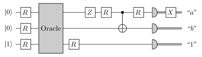
Figure 1: A circuit diagram for the four-element Grover algorithm, based on the figure in Box 6.1 of Nielsen and Chuang (2000). The top two qubits are the data qubits, initialized in state $|0\rangle|0\rangle$, while the bottom qubit is the ancilla qubit, initialized in state $|1\rangle$. The boxes labeled $R$ and $Z$ represent the one-qubit Hadamard and Pauli $\sigma_{Z}$ gates, respectively. The cnot is denoted by the usual symbol, while the gray half-circles represent one-qubit measurements in the computational basis, whose output appears on the classical output wires (double lines). The final $X$ gate represents the classical not required to put the output into the correct form. The measurement always gives “1” on the ancilla qubit, while the data qubits give “$a$” and “$b$”. It is straightforward to show that, in principle, $ab$ is the state marked by the oracle.

For the remainder of this paper, we restrict our attention to the case where the number of elements in the search space is $N=4$. In that case, the number of repetitions specified by Eq. (1) is exactly one. A simplified circuit based on the algorithm described above is shown in Fig. 1. It can be verified directly that this circuit, using only one oracle call, gives the correct answer with probability 1, compared to the average of 2.25 oracle calls that must be made with a classical circuit. For example, if the solution is 10, then the output of the circuit is $a=1$ and $b=0$.

II.2 Implementing the oracle

An oracle is a quantum circuit that recognizes solutions to a given problem. For example, suppose we wish to solve a version of the traveling salesman problem, where the goal is to find a route visiting a given collection of cities that is shorter than some specified length $L$. Although it is in general hard to find such a route, it is easy to recognize whether a proposed route solves the problem: simply add up the total distance the salesman would travel on the proposed route, and compare it to $L$.

Specifically, an oracle is a circuit that, given an input consisting of a potential solution to a problem, flips the sign of an ancilla qubit if and only if the input is a solution to the problem. Since the only action of the oracle is to recognize solutions, its internal structure is unimportant in a test of the algorithm itself. Thus, for our purposes, the choice of oracle is arbitrary, and may be chosen to be as simple as possible.

Although the internal workings of the oracle are unimportant for the purposes of testing the algorithm, the complexity of implementing some oracle must be included to characterize the difficulty of performing the experiment. A simple implementation of an oracle marking one of four states is a Toffoli gate, with the control qubits negated where necessary to specify any of the states 00, 01, 10, or 11 (see the left-hand side of Fig. 2 for the example where the marked state is 10).

Figure 2: The circuit on the left shows the beginning of the Grover circuit with an example oracle (inside the dashed box) marking the item 10. We have implemented the oracle using a variant of the Toffoli gate, where the state of the third qubit is flipped when the first two qubits are in the state $|10\rangle$, as indicated by the closed and open circles on the control qubits. We have moved the measurement on the third qubit forward since it plays no further role in the algorithm. In the text, we show that this circuit is in fact equivalent to the simplification on the right, where the Toffoli has been replaced by a controlled-$Z$ (csign) operation followed by an $X$ on the appropriate qubit.

If the marked state is 10, the action of the oracle on the three qubits is to take the state $(|00\rangle+|01\rangle+|10\rangle+|11\rangle)(|0\rangle-|1\rangle)$ to

$$\begin{split}(|00\rangle+|01\rangle+|11\rangle)(|0\rangle-|1\rangle)+|10\rangle(|1\rangle-|0\rangle)\\ =(|00\rangle+|01\rangle-|10\rangle+|11\rangle)(|0\rangle-|1\rangle)\end{split}$$ (2)

(omitting the normalization). Thus the oracle simply has the effect of flipping the sign of the marked state. The ancilla is not used again, so it can be discarded at this point.

Toffoli gates are difficult to implement in LOQC because there is no known way to implement one without using several cnots. However, for our purposes, a full Toffoli gate is not required because the ancilla qubit plays such a limited role. The two-qubit circuit on the right-hand side of Fig. 2 illustrates this for the case where the marked state is 10. A single controlled-$Z$ (csign) gate that flips the sign of the $|11\rangle$ state, followed by $X$ gates to move the minus sign to the appropriate state, has the same action as the original oracle.

A simplified circuit to implement the four-element Grover algorithm is given in Fig. 3. This is the circuit that we will work with for the remainder of this paper.

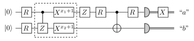
Figure 3: Inserting the simplified oracle of Fig. 2 into the circuit of Fig. 1 gives this circuit. Note that the marked state is specified inside the oracle (the dashed box) by the values of $x_{1}$ and $x_{2}$ used to determine whether or not the $X$ gates are applied. (Note that addition in the exponent of the $X$ gates is modulo 2.) Under ideal circumstances, the output of the circuit is $a=x_{1}$ and $b=x_{2}.$

III LOQC with polarization encoding

In LOQC, qubits are encoded in dual rail logic Knill et al. (2001a): Two modes $A$ and $B$ are used, and logical $|0\rangle$ and $|1\rangle$ are encoded as $|1\rangle_{A}|0\rangle_{B}$ and $|0\rangle_{A}|1\rangle_{B}$, respectively. The modes may represent two different spatial modes, or two different polarization modes of a single spatial mode.

In practice, it is likely that polarization-encoded qubits will be used, so that logical $|0\rangle$ and $|1\rangle$ are encoded as $|H\rangle$ and $|V\rangle$, respectively, where $H$ and $V$ refer to horizontal and vertical polarization one-photon states of the same spatial mode. The main reasons for this are (1) it significantly simplifies the implementation of the cnot gate (see below), (2) it allows one-qubit gates to be implemented using only waveplates and phase delays rather than beamsplitters and interferometers, and (3) it reduces the effects of noise by ensuring that, unlike with spatial encoding, both states follow the same path on the quantum wires between gates. In this section we describe in some detail the construction of one-qubit gates and cnots in polarization-encoded LOQC.

III.1 One-qubit gates

Gate	Optical element
$e^{i\theta}I=e^{i\theta}\left[\begin{smallmatrix}1&0\\ 0&1\end{smallmatrix}\right]$	phase delay of $-\theta$
$R=\frac{1}{\sqrt{2}}\left[\begin{smallmatrix}1&1\\ 1&-1\end{smallmatrix}\right]$	waveplate with $\phi=180^{\circ}$, $\alpha=-67.5^{\circ}$
$T=\left[\begin{smallmatrix}1&0\\ 0&e^{i\pi/4}\end{smallmatrix}\right]$	waveplate with $\phi=45^{\circ}$, $\alpha=90^{\circ}$
$X=\left[\begin{smallmatrix}0&1\\ 1&0\end{smallmatrix}\right]$	waveplate with $\phi=180^{\circ}$, $\alpha=-45^{\circ}$
$Z=\left[\begin{smallmatrix}1&0\\ 0&-1\end{smallmatrix}\right]$	waveplate with $\phi=180^{\circ}$, $\alpha=90^{\circ}$
$Y=\left[\begin{smallmatrix}0&-i\\ i&0\end{smallmatrix}\right]$	2 waveplates and a phase delay: $(e^{i\pi/4}I)XZ$

.

Table 1: Various one-qubit gates and their implementation in polarization-encoded LOQC. $\alpha$ and $\phi$ refer to the angle of the slow axis to the horizontal and the relative phase added to light parallel to the slow axis, respectively. Note that $T$ requires a waveplate with a relative delay of one eighth of a wavelength.

To our knowledge, no complete description of how to implement basic quantum gates with polarization encoding has been given in the literature, so we provide one here. For one-qubit gates, waveplates and phase delays are sufficient. A waveplate with slow axis $|H^{\prime}\rangle$ and fast axis $|V^{\prime}\rangle$ has action

$$\begin{split}|H^{\prime}\rangle&\to e^{i\phi}|H^{\prime}\rangle\\ |V^{\prime}\rangle&\to|V^{\prime}\rangle,\end{split}$$ (3)

where $\phi$ is the resulting relative phase difference. Special cases in common use are the half and quarter waveplates, with $\phi$ equal to half and a quarter of a wavelength, respectively. Now suppose $|H^{\prime}\rangle$ is rotated counter-clockwise (with respect to the direction of travel of the light) by an angle $\alpha$ from $|H\rangle$. If the input state is $\left[\begin{smallmatrix}h\\ v\end{smallmatrix}\right]\equiv h|H\rangle+v|V\rangle$, then the output is given by

$$\left[\begin{matrix}e^{i\phi}\cos^{2}\alpha+\sin^{2}\alpha&(e^{i\phi}-1)\cos\alpha\sin\alpha\\ (e^{i\phi}-1)\cos\alpha\sin\alpha&e^{i\phi}\sin^{2}\alpha+\cos^{2}\alpha\end{matrix}\right]\left[\begin{matrix}h\\ v\end{matrix}\right].$$ (4)

Special cases of this transformation for common one-qubit gates are set out in Table 1. The Hadamard and $\pi/8$ gates, labeled $R$ and $T$ in the table, are a universal set for one-qubit quantum computation (Boykin et al. Boykin et al. (2000)), and so any one-qubit gate can be obtained by a sequence of waveplates, although it is convenient to allow phase delays as well. In the Grover circuit, the only one-qubit gates used are the $R$, $X$, and $Z$ gates, and thus we only require half waveplates.

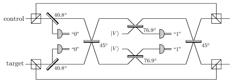
Figure 4: The simplified KLM csign of Ralph et al. (2002a). The top rail contains the control qubit and the bottom rail contains the target qubit, both encoded in the polarization of a single photon. A square with a diagonal line across it represents a polarizing beamsplitter. By convention, we always assume that the horizontal polarization is 100% reflected while the vertical polarization is 100% transmitted. So, for example, after the first polarizing beamsplitters, the topmost rail contains the horizontally polarized component of the control qubit. A thin rectangle represents an ordinary beamsplitter, with a sign change for the mode reflected from the thick black side and reflectivity given by the cosine of the angle written next to it. (If the input modes to a beamsplitter are $|a\rangle_{\text{in}}$ and $|b\rangle_{\text{in}}$, with the $b$ mode receiving the sign change and with reflectivity given by $\cos x$, then the outputs are $\cos x|a\rangle_{\text{out}}+\sin x|b\rangle_{\text{out}}$ and $\sin x|a\rangle_{\text{out}}-\cos x|b\rangle_{\text{out}}$.) The circuit uses two vertically polarized ancilla photons. It succeeds if the first two measurements both count 0 photons and the second two measurements both count 1 photon.

III.2 Two-qubit gates

Since the publication of the original LOQC scheme of KLM Knill et al. (2001a), many simplifications of their csign gate have been developed, with varying trade-offs between simplicity and functionality. The different types may be divided into two classes, those that are scalable and those that are not. In this section, we describe both types. (Note that the cnot and csign gates are related by conjugation by Hadamards on the target bit, i.e. $\textsc{cnot}=(I\otimes R)\textsc{csign}(I\otimes R)$. Therefore, in the context of LOQC where one-qubit gates are relatively straightforward, these two gates are practically equivalent, and we will use the two almost interchangeably.)

III.2.1 Scalable two-qubit gates

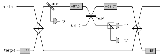
Figure 5: A further simplified (but still scalable) polarization-encoded KLM csign. A gray rectangle containing “$x^{\circ}$” represents a half waveplate with slow axis at an angle of $x^{\circ}$ to the horizontal polarization. See Table 1 for the corresponding one-qubit gates. This circuit works similarly to the previous one (Fig. 4), but it takes fuller advantage of the orthogonality of the polarization states. For a full description, see the text.

The KLM scheme Knill et al. (2001a) has two properties that at first appear contradictory: the LOQC csign is non-deterministic, but it is used to do computations in a scalable manner. The non-deterministic nature of the KLM csign is essential to engineer a two-photon interaction without using highly nonlinear materials, but it poses a problem: if its success probability is $\epsilon<1$, then the success probability of a circuit with $n$ csigns is $\epsilon^{n}$ — it decreases exponentially with $n$. A solution to this problem is the technique of gate teleportation described by Nielsen and Chuang Nielsen and Chuang (1997) and Gottesman and Chuang Gottesman and Chuang (1999). This technique allows the gates to be prepared as an offline resource, and then “teleported in” whenever required for a computation. KLM showed that the teleportation step can be made near-deterministic using a sufficiently large number of repetitions. This technique is unlikely to be used in early experiments, however, because the extra difficulty involved in teleporting gates will more than cancel out the advantages of increasing the success probability when the number of csigns is small.

An essential feature required to make this work is that it must be possible to determine when the gate has succeeded. The KLM cnot has this property — although it only succeeds 1 time in 16, whether or not it has succeeded is determined by the outcomes of measurements on ancilla photons. We use the term scalable to describe a csign (or cnot) that has the property that it is known when it succeeds.

In this paper, we will not work directly with the KLM csign since there are simpler alternatives, such as the closely related simplification proposed by Ralph et al. Ralph et al. (2002a) and the substantial modification proposed by Knill Knill (2002). There is also a promising alternative approach using entangled ancillas discovered by Pittman, Jacobs and Franson Pittman et al. (2001) that we will not consider further here. We focus on the csign of Ralph et al., shown in Fig. 4.

In fact, there is a further, substantial simplification to this circuit that is achieved by making fuller use of the polarization encoding, resulting in the circuit in Fig. 5. This gate still requires two ancilla photons. However, it uses fewer detectors, beamsplitters, and polarizing beamsplitters, and eliminates two interferometers. Its effect on qubit states is unchanged, up to an unimportant overall phase of $-1$. If we denote the beamsplitter reflectivities as $\eta_{1}\equiv 5-3\sqrt{2}$ and $\eta_{2}\equiv(3-\sqrt{2})/7$ (which are approximated as $\cos 40.8^{\circ}$ and $\cos 76.9^{\circ}$ in the diagram), then the action of the gate is the following:

$$\begin{split}&|00\rangle\to\sqrt{\eta_{1}\eta_{2}}(2\eta_{2}-1)|00\rangle=-\sqrt{p}|00\rangle\\ &|01\rangle\to\eta_{1}(3\eta_{2}^{2}-2\eta_{2})|01\rangle=-\sqrt{p}|01\rangle\\ &|10\rangle\to\sqrt{\eta_{1}\eta_{2}}(2\eta_{2}-1)|00\rangle=-\sqrt{p}|10\rangle\\ &|11\rangle\to\eta_{2}|11\rangle=\sqrt{p}|11\rangle\\ \end{split}$$ (5)

where the success probability $p$ is given by $p\equiv\eta_{2}^{2}=(11-6\sqrt{2})/49\approx 0.05$. Thus the gate works approximately 1 out of every 20 attempts. For the remainder of this paper, we will refer to this gate simply as a “scalable csign”.

III.2.2 Coincidence-basis two-qubit gates

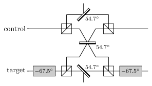
Figure 6: The coincidence-basis cnot of Hofmann and Takeuchi (2002); Ralph et al. (2002b). All three beamsplitters have the same reflectivity $1/3\approx\cos 54.7^{\circ}$. It can be turned into a csign by removing the two halfwave plates. Note that it is not necessary to have detectors on the reflected modes of the topmost and bottommost beamsplitters (even though measuring a photon in either of these modes would signal a failure), since other failures of this gate are undetectable until the end of the computation. The gate has worked if exactly one photon is found in each rail.

An even simpler, but non-scalable cnot was discovered by Hofmann and Takeuchi Hofmann and Takeuchi (2002) and Ralph et al. Ralph et al. (2002b). It succeeds 1 time in 9, but it only works in the coincidence basis, i.e. when the results of the whole computation are selected to contain an allowed distribution of photons among detectors. We call this a coincidence-basis cnot. See Fig. 6. This circuit has been designed so that if exactly one photon is measured in the top rail (in either polarization), and one in the bottom rail, it has worked with certainty. Otherwise, the result is discarded and the experiment is repeated. It cannot in general be followed by further two-qubit gates, as it is possible for a later gate to mask a failure. Thus it cannot be used to do scalable quantum computation.

The useful purpose served by this gate (as well as the coincidence-basis gate of Pittman et al. (2003)) is as a simpler intermediate step before the full complexity of a scalable cnot. In a general circuit, it may be possible to replace one or more scalable cnots with a coincidence-basis cnot, thereby significantly reducing the complexity of circuits containing a few cnots. In the following sections on constructing optical circuits to perform the four-element Grover algorithm, we will see some of these ideas in action.

IV The two-qubit Grover in LOQC

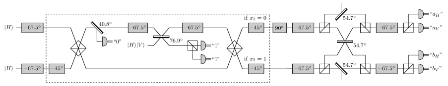
Figure 7: An optical implementation of Grover’s algorithm on four elements based on the circuit in Fig. 3. The oracle part is contained in the dashed box. This circuit is essentially the concatenation of the circuits for the scalable csign (Fig. 5) and the coincidence-basis cnot (Fig. 6), together with a few extra waveplates. The output of the circuit is discarded unless the first measurement counts 0 photons, the second two measurements both count 1 photon, and one photon is found in each pair of detectors at the end, i.e. $a_{H}+a_{V}=b_{H}+b_{V}=1$. Note that we have omitted the final correcting not gate on the classical output in this diagram, but it should still be done. For example, if the oracle marks state 10, then the algorithm has successfully identified the marked state if measurements return $a_{H}=1$, $a_{V}=0$, $b_{H}=1$, $b_{V}=0$.

A simplified circuit for the four-element Grover algorithm was given in Fig. 3. In Fig. 7, this circuit is translated directly into an optical circuit, using the prescriptions and circuits of the previous section.

The circuit, which succeeds one time in approximately $180=20\times 9$ (the product of the number of attempts per success for each cnot), uses 10–12 half waveplates, 5 beamsplitters (2 of which must be modematched), 9 polarizing beamsplitters (4 of which must be modematched), 4 photons that must be simultaneously produced in desired polarization states, and 7 single-photon detectors. The second cnot can be done in the coincidence basis since there are no interactions between the two qubits following it. Therefore, if the final measurement contains an allowed distribution of photons (exactly one in the top two detectors and one in the bottom two detectors), we know that the second cnot worked, which is sufficient for our purposes here.

However, it is important to note that the output of this circuit (before the measurement) could not be used to do further calculations because of the uncertainty in the outcome of the second cnot. If, for example, there were two photons in the top rail after the second cnot, the system’s state would no longer be in the “qubit space”. A third cnot might bring the system back into the qubit space, but it is unlikely to have performed the transformation we expected. In this case, the overall circuit fails, but we have no way of detecting the failure (except to compare with the answer that we can calculate by hand for this simple case).

To ensure reliability for further calculations, the second cnot should be replaced by a scalable cnot. The optical circuit for this case would work one time in 400, and would contain on the order of 14–16 waveplates, 8 polarizing beamsplitters (6 of which would be modematched), 4 ordinary beamsplitters (2 of which would be modematched), 6 photons produced in desired polarization states simultaneously, and 10 single-photon detectors. This would be considerably more difficult to achieve experimentally. Since we are (in principle) guaranteed to be in the qubit space at the end of this circuit, the output of each pair of detectors should contain exactly one photon. Therefore, it is possible to simplify the final detection process by simply blocking out one of the polarizations (horizontal, say), and then looking to see if a photon is detected. This would reduce the number of polarizing beamsplitters to 6 and the number of detectors to 8, at the cost of introducing two polarization filters. However, in practice the number of photons at the output will sometimes be incorrect. Thus, the increase in simplicity would have to be weighed against the failures that would go undetected.

V Simplifications

By far the most difficult aspect of the experiments just described is implementing the scalable csigns. However, the csign in the oracle is only used in a very restricted way, and it turns out that we can replace it with a much simpler circuit. Since only one input state is ever used, namely $(|H\rangle+|V\rangle)(|H\rangle+|V\rangle)$, only one state is ever output from the csign, namely $|HH\rangle+|VH\rangle+|HV\rangle-|VV\rangle$. (We will continue to neglect normalization constants.) If a source of entangled input states were available, then the csign could be replaced. In optics, such a source is in fact readily available: a parametric down conversion source can be used to produce the state $|HH\rangle+|VV\rangle$, which can be converted into our desired state by a Hadamard gate on the first qubit, $|H\rangle\to|H\rangle+|V\rangle$, $|V\rangle\to|H\rangle-|V\rangle$. Using this fact, a much simplified version of Grover’s algorithm is presented in Fig. 8.

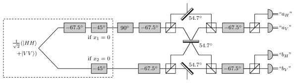
Figure 8: Grover’s algorithm using a parametric down conversion input. This circuit works similarly to the previous one, but the oracle is no longer demarcated from the initial part of the circuit. The dashed box in this figure now contains both the oracle and the initialization to the state $|HH\rangle+|VV\rangle$. The advantage of this circuit is that it makes use of a natural source of optical entanglement (parametric down conversion) to replace the very difficult scalable csign. The outputs from this circuit are accepted under the same conditions as the previous circuit ($a_{H}+a_{V}=b_{H}+b_{V}=1$), and the final classical not has again been omitted.

The simplicity of this circuit compared with the previous one is emphasized by comparing the number of components. This circuit works one in every 9 attempts, and requires 6–8 waveplates, 6 polarizing beamsplitters (of which 2 must be modematched), 3 ordinary beamsplitters (1 of which must be modematched), 2 photons which are produced as the output of a parametric down-conversion source, and 4 single-photon detectors.

What have we traded for this enormous gain in simplicity? It turns out that we have compromised the versatility of the algorithm. Most significantly, the oracle is no longer easily replaceable. In principle, the oracle should be a ‘”plug-in” component able to have many different forms corresponding to different potential problems. In this simplified scheme, however, we have obscured the line between the oracle and non-oracle parts of the circuit, making it difficult to see how to make the circuit solve a problem using a different oracle. In Fig. 8, a dashed box outlines the “oracle” part of the circuit for comparison with the previous diagrams, but there is in fact no clear line dividing the oracle from the earlier part of the circuit.

This change affects how the circuit could be used. One example is demonstrating the variation in the success probability of Grover’s algorithm as a function of the number repetitions of steps (3)–(6) described in Sec. II. In the circuit in Fig. 7, the oracle can be reused with some small changes. On the other hand, in Fig. 8, this is not possible — the “oracle” can only be used once.

VI Figures of merit

An important question that has so far not been addressed is what the appropriate figures of merit are for this experiment. There are two related but distinct notions of success here. The first is to what extent the actual goal of Grover’s algorithm has been achieved, i.e. how successfully the experiment distinguishes between the four different oracles. The second is how similar the actual operation of circuit is to the ideal operation. This second notion is important for using these experiments as tests of the ability to combine the basic elements of quantum computation. It is clearly related to the first — if the experiment cannot reliably distinguish between the oracles, then the actual behavior of the circuit must be very far from the ideal operation.

In order to be able to compare experiments (and also to optimize the performance of a particular experimental setup), we need to be more precise about how to measure the success of these experiments. We suggest calculating figures of merit reflecting each of the two notions of success described above. The first is simply to measure the distinguishability of the distribution of measurement results output by the circuit for different oracles. For example, suppose that for the oracle marking the state $00$, the results $00$, $01$, $10$, and $11$ occur with probabilities $p_{00}\equiv\{0.9,0.04,0.02,0.04\}$, while the corresponding results when the oracle marks state $10$ are $p_{10}\equiv\{0.01,0.08,0.8,0.11\}$. A simple indicator of the distinguishability of these two distributions is their fidelity

$$F(p_{00},p_{10})\equiv\sum_{x}\sqrt{p_{00}(x)p_{10}(x)}$$ (6)

where $x$ ranges over the measurement outcomes $00,\dots,11$ and $p_{ab}(x)$ is the probabilities of obtaining result $x$ given that the oracle marked state $ab$. This quantity has the property that it is 1 precisely when the two distributions are identical and 0 precisely when the two distributions are non-overlapping, that is, when the set of results for which the first distribution is non-zero has no elements in common with the set of results for which the second distribution is non-zero.

In the context of Grover’s algorithm, it is desirable to make the fidelity between the distributions arising from each pair of oracles as large as possible. (For an introduction to the fidelity, see, for example, Fuchs (1996); Nielsen and Chuang (2000). The relationship of the fidelity to distinguishability is explored in Wootters Wootters (1981) and Fuchs (1996).)

The second figure of merit is related to the similarity of the actual operation implemented ${\cal E}$ to the desired unitary $U$. $U$ is obtained by simply multiplying together the circuit elements in Fig. 3. ${\cal E}$, on the other hand, must be determined experimentally. Ideally, ${\cal E}$ should be determined precisely using a method such as quantum process tomography (Chuang and Nielsen Chuang and Nielsen (1997) and Poyatos, Cirac, and Zoller Poyatos et al. (1997)). Although process tomography can be done using only product-state inputs and one-qubit measurements, it requires an enormous number of runs of the experiment since the output states resulting from 16 different input density matrices must be determined via quantum state tomography.

A less stringent, but much more easily calculated, criterion is that the probability distributions for each oracle should be close to the ideal distributions. Again, it is desirable to have the fidelity of the actual distribution to the ideal distribution for each oracle as close to 1 as possible.

VII A hierarchy of experiments

This collection of different implementations of the same algorithm could be used as the basis for a series of experiments, each building on the last, each more complicated than the last, each demonstrating improved quantum control. For example, once a basic coincidence-basis cnot is working, it would be relatively simple to add a small number of waveplates and a source of entangled photons to do the circuit in Fig. 8. Once a scalable cnot is achieved, these two different cnot circuits could be combined to do the more complicated implementation of Grover’s algorithm in Fig. 7, demonstrating the ability to combine a scalable cnot with further non-trivial quantum computations. Finally, in the more distant future, the implementation using two scalable cnots would make a good testing ground for techniques for combining LOQC components.