Accuracy of quantum-state estimation utilizing Akaike’s information criterion

Abstract

We report our theoretical and experimental investigations into errors in quantum state estimation, putting a special emphasis on their asymptotic behavior. Tomographic measurements and maximum likelihood estimation are used for estimating several kinds of identically prepared quantum states (bi-photon polarization states) produced via spontaneous parametric down-conversion. Excess errors in the estimation procedures are eliminated by introducing a new estimation strategy utilizing Akaike’s information criterion. We make a quantitative comparision between the errors of the experimentally estimated states and their asymptotic lower bounds, which are derived from the Cramér-Rao inequality. Our results reveal influence of entanglement on the errors in the estimation. An alternative measurement strategy employing inseparable measurements is also discussed, and its performance is numerically explored.

I Introduction

One of the central features of quantum mechanics is that it does not allow to simultaneously obtain whole information about an individual quantum system without errors MP1995 . The Holevo bound on the accessible information and the no-cloning theorem are the prominent manifestations of the restrictions on acquiring information from quantum systems NCtext2000 , and these restrictions culminate in quantum cryptography NCtext2000 .

However, there are no obstacles to estimate all aspects of quantum states in a series of distinct measurements on identically prepared particles by quantum state tomography NCtext2000 ; Leonhardt1997 . The pioneering experimental demonstration of this method has been accomplished by Smithey, et al. SBRF1993 . They determined a Wigner function for vacuum and pulsed squeezed-vacuum state of a spatial-temporal mode using homodyne tomography. Schiller, et al. SBPMM1996 applied this method to a estimation of a density matrix (in the number state representation) for squeezed vacuum state of two spectral components. In this experiment, the spectacular even-odd oscillations in the photon-number distribution was observed. Recently, Lvovsky et al. LHABMS2001 and Bertet et al. BAMOMBRH2002 have respectively succeeded in reconstructing a Wigner function for single-photon Fock state of a travelling spatial-temporal mode and that of a intra-cavity mode. Both estimated Wingner functions showed a dip reaching classically-impossible negative values around the origin of the phase space. For the polarization degree of freedom of electromagnetic field, White et al. WJEK1999 used quantum state tomography, for the first time, to characterize non-maximally entangled states produced from a spontaneous-down-conversion photon source. Kwiat et al. utilized this method for the verification of decoherence-free characteristic of a particular entangled state KBAW2000 , and for the demonstration of hidden non-locality of entangled mixed states KBSG2001 .

In spite of these splendid experimental achievement with quantum state tomography, statistical errors in estimating quantum states have been paid minor attention so far. Statistical analyses of errors in quantum-state estimation should not be undervalued. Since any outcomes of measurements are represented as a random variable in quantum mechanics, statistical analyses of their errors may reveal profound rule for acquiring information from quantum system. Moreover, such analyses may also lead to the development of quantum information technology, which requires us to faithfully prepare several kinds of quantum states NCtext2000 , and to the improvement of the sensitivity for various kinds of precision measurements, which is limited by quantum noises Phase ; Polarization .

In this article, we report our theoretical and experimental analyses of errors in quantum state estimation putting a special emphasis on their asymptotic behavior. In particular we focus on the estimation of the state of two qubits (two 2-level quantum systems). The two-qubit system in 4-dimensional Hilbert space is the simplest one where the peculiar characteristic of quantum mechanics, entanglement, is activated. Since entanglement plays the critical role in the mysterious phenomena in the quantum world Bell ; BWMEWZ1997 ; QCrypto2000 , it is interesting to ask whether entanglement affects accuracy of the estimation. Various kinds of two qubits (including entangled states) are practically realizable as polarization states of bi-photon produced via spatially-nondegenerate, type-I spontaneous parametric down-conversion (SPDC) WJEK1999 ; KBAW2000 ; KBSG2001 ; KWWAE1999 ; JKMW2001 ; WJMK2001 ; NUTMN2002 . The procedure to estimate the state of two qubits has been well established by James, Kwiat, Munro and White JKMW2001 . Thus, in our experiments, we followed the above methods for producing the ensembles of the bi-photon polarization states, for measuring them, and for estimating their density matrices.

The main purpose of this article is to quantitatively show the limit on accuracy of quantum-state estimation. We demonstrate that the accuracy depends on state to be estimated and also measurement strategy. In order to do that, we introduce a new strategy of quantum-state estimation utilizing Akaike’s information criterion (AIC) Akaike1974 for eliminating numerical problem in the estimation procedures especially in estimating (nearly) pure quantum states. While number of parameters used for characterizing density matrices of quantum states is fixed in the conventional estimation strategies JKMW2001 ; BDPS1999 ; RHJ2001 , the number is varied in the new strategy for eliminating redundant parameters. Consequently, we can quantitatively compare experimentally-evaluated errors in the estimation with their asymptotic lower bound derived from the Cramér-Rao inequality without bothering about the delicate numerical problem accompanying the redundant parameters. It is shown that the errors of the experimental results nearly achieve their lower bounds for all quantum states we examined. Moreover, owing to the reduction of the parameters, the AIC based new estimation strategy makes the lower bounds slightly decreased.

Our results reveal that when measurements are performed locally (i.e., separately) on each qubit, existence of entanglement may degrade the accuracy of estimation. Thus, while the measurements in our experiments are local ones, we numerically examine the performance of an alternative measurement strategy, which includes inseparable measurements on two qubits.

The remainder of the article is organized as follows. In Sec. II, we show our experimental analyses of errors in estimating density matrices as a function of the ensemble size, i.e., as varying data acquisition time. In Sec. III, we present a prescription for calculating the asymptotic lower bounds on the errors in terms of fidelity and show that in the asymptotic region, the errors should be decreasing as inversely proportional to the ensemble size. Then we compare the lower bounds with the experimental results. In Sec. IV, a new strategy of quantum state estimation utilizing Akaike’s information criterion is introduced, and the accuracy of the state estimated by this new strategy is presented. In Sec. V, the alternative measurement strategy for two qubits, which employs inseparable measurements, is numerically explored. Section VI summarizes this article. In the Appendix, we briefly review tomographic measurements and maximum likelihood estimation for estimating two qubits, and derive the Cramér-Rao lower bound on the errors in the estimation.

II experiment

II.1 experimental setup

For experimentally producing various quantum states of two qubits, we use the method to create the various polarization states of bi-photon via spatially-nondegenerate, type-I spontaneous parametric down-conversion (SPDC). The method was invented by Kwiat et al. KWWAE1999 and applied to the various experiments WJEK1999 ; JKMW2001 ; KBAW2000 ; KBSG2001 ; WJMK2001 ; NUTMN2002 .

Figure 1: Experimental setup for producing various polarization states of bi-photon and measuring them.

A rough sketch of the experimental setup is shown in Fig. 1. Two thin (0.13mm) beta-barium borate ($\beta$-$BaB_{2}O_{4}$, BBO) crystals, which are cut for satisfying the type-I phase matching, are adjacent so that their optical axes lie in the planes perpendicular to each other. Inside the crystals, the third harmonic beam (wave length: 266nm, average power: 190mW) of the mode-locked Ti:Sapphire laser (pulse duration: 80fs, repetition rate: 82MHz) -we will call it pump beam- is slightly converted into the frequency-degenerate, but spatially-nondegenerate (opening angle: $3^{\circ}$) bi-photon (wave length: 532nm) via SPDC. This configuration of the setup makes it possible to produce various polarization states of bi-photon (including entangled states) by adjusting the pump beam polarization with a half-wave plate (HWP) WJEK1999 ; KWWAE1999 , by modifying the relative time delay between the horizontal and vertical components of the pump beam with a pre-compensator (which consists of quartz plates and a variable wave plate (WP)) NUTMN2002 , and by inserting decoherers (two de-polarizers) into one of the paths of the down-converted photons KBAW2000 ; KBSG2001 ; WJMK2001 , as shown in Fig. 1. We produced three particular quantum states, the very noisy mixed state (VNMS), the almost pure and separable state (APSS), and the highly entangled state (HES) for inspecting influence of the various characteristics (e.g., entropy and entanglement) of the states on the accuracy of the estimation.

The produced polarization states of bi-photon were estimated by tomographic measurements JKMW2001 ; WJEK1999 and maximum likelihood estimation (MLE) JKMW2001 ; BDPS1999 ; RHJ2001 . These procedures are reviewed in Appendices A.1 and A.2. In tomographic measurements, the coincidental detection events (within 6ns) on both single-photon detectors (HAMAMATSU H7421-40) were counted by using the time interval analyzer (YOKOGAWA TA-520) during the data acquisition time $t$ at each polarizer’s setting (i.e., projector) $|m_{\nu}\rangle\langle m_{\nu}|$ (which was determined and varied by the half-wave plate (HWP), the quarter-wave plate (QWP), and the polarizer (Pol) on each path of the produced photons). For investigating ensemble size-dependence of the accuracy, we varied the data acquisition time of each measurement $t$ as 0.2s, 0.5s, 1.0s, 2.0s, and 5.0s. The typical single counting rate was about 30000c/s with the dark counting rate of about 300c/s. The typical coincidence counting rate was roughly 500c/s with the accidental coincidence counts being below 1% of the genuine coincidence counts. For eliminating the ambient photons, we used the interference filters (FWHM: 8nm) (see Ref. NUTMN2002 , for more detailed information).

II.2 experimental procedure

In order to assess the accuracy of the estimation, we repeated the measurements and estimation procedures 9 times for each state and each ensemble size. Here, as noted in Appendix A.2, the density matrix of the two-qubit(2 two-level quantum state) can be written as

$$\rho_{\Theta}=\frac{T_{\Theta}T_{\Theta}{}^{\dagger}}{\mathop{\mathbf{Tr}}\nolimits[T_{\Theta}T_{\Theta}{}^{\dagger}]},$$

which satisfies the positivity condition and the trace condition for density matrices JKMW2001 ; BDPS1999 ; see Appendix A.2. As a result of the 9 identical trials, we had 9 slightly different density matrices $\{\rho_{\hat{\Theta_{i}}}\}_{i=1}^{9}$. The differences of these states might stem not only from the statistical errors but also from the experimental systematic ones. For reducing the systematic errors, we restricted our data acquisition time, $t$, at each polarizer setting up to $t=5s$, so as to keep the experimental condition unchanged (especially, to keep the pump power constant during whole data acquisition time $t\times 16$ measurements).

Then we evaluated the accuracy of the estimation in terms of the average fidelity between the true state $\rho_{\Theta_{0}}$ and each estimated state $\{\rho_{\hat{\Theta_{i}}}\}_{i=1}^{9}$, i.e.,

$$F(\rho_{\Theta_{0}},\rho_{\hat{\Theta}})\approx\frac{1}{9}\sum_{i=1}^{9}F(\rho_{\Theta_{0}},\rho_{\hat{\Theta_{i}}}),$$ (1)

where the fidelity $F(\rho_{1},\rho_{2})$ is equal to $\mathop{\mathbf{Tr}}\nolimits[\sqrt{\sqrt{\rho_{1}}\rho_{2}\sqrt{\rho_{1}}}\,]$ NCtext2000 ; Jozsa1994 ; BCFJS1996 . As the true state $\rho_{\Theta_{0}}$ for each of our concerned three states (the VNMS, the APSS, and the HES), we employed a state which was estimated by the MLE using the whole data acquired for each state. This means that the effective data acquisition time for determining the true state amounts to $t$=0.2s$\times$9-trial+0.5s$\times$9-trial+1.0s$\times$9-trial+2.0s$\times$9-trial+5.0s$\times$9-trial=78.3s. Later on we use these three true states as sources to produce artificial 16 coincidence-count data for the numerical simulations. These simulations are performed without considering any systematic errors. Thus we can evaluate to what extent the systematic errors affect the total errors.

II.3 experimental results

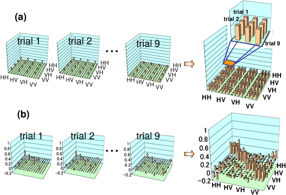
Figure 2: To see fluctuation of the estimation, we use a matrix shown in the most right-hand side of (a). This matrix has $12\times 12$ elements and is composed of 9 matrices ($4\times 4$ matrix) shown in the left-hand side of (a). Each of the 9 matrices is the real part of the density matrix estimated by each trial. The relation between the elements of $12\times 12$ matrices and those of the $4\times 4$ matrices is illustrated in (a). As an example, the $12\times 12$ matrix and the constituent $4\times 4$ density matrices for the VNMS are shown in (b). The bases of the density matrices are $|HH\rangle$, $|HV\rangle$, $|VH\rangle$ and $|VV\rangle$ (these notations are defined in Appendix A.1). In this way, fluctuations of estimated density matrices can be visualized.

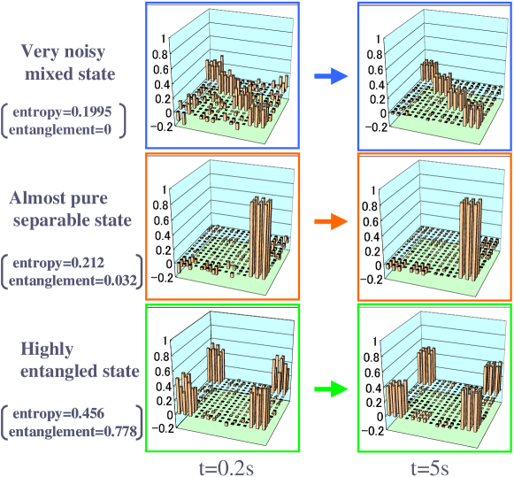
Figure 3: The $12\times 12$ matrix (which is composed of 9 density matrices ($4\times 4$)) for the three states, i.e., the VNMS, the APSS, and the HES, for two different data acquisition time, $t=0.2s$ (left) and $t=5.0s$ (right). The detailed explanation for each element of the matrices is provided in Fig. 2. Entropy (von Neumann entropy) and entanglement (entanglement of formation) of each resulting true state (which is obtained by using the whole data as mentioned in the text) is also presented. Note that only the real parts of the density matrices are exhibited, because the imaginary parts are quite small compared with the real parts.

To visualize fluctuation of the estimation, we use a matrix, which is explained in detail in Fig. 2. This matrix has $12\times 12$ elements and is composed of the 9 matrices ($4\times 4$ matrix), each of which is the real part of the density matrix estimated by each trial. Figure 3 shows the matrices for three states (i.e., the VNMS, the APSS, and the HES) for two different data acquisition time, $t=0.2s$ and $t=5.0s$. Here the bases of the density matrices are $|HH\rangle$, $|HV\rangle$, $|VH\rangle$ and $|VV\rangle$ (these notations are defined in Appendix A.1). Entropy (von Neumann entropy NCtext2000 ) and entanglement (entanglement of formation NCtext2000 ) of each resulting true state, which is obtained by using the whole data as mentioned before, is also shown in Fig. 3. Note that the each density matrices had little imaginary parts in all cases, thus they are not presented. We can observe that the fluctuation of each element is reduced as the data acquisition time, $t$, becomes long (from 0.2s to 5.0s) in all three states.

In Fig. 4, the fluctuations of the estimated density matrices are quantitatively shown in terms of the average fidelities between the true state $\rho_{\Theta_{0}}$ and the estimated states $\{\rho_{\hat{\Theta_{i}}}\}_{i=1}^{9}$ as a function of the ensemble size. The ensemble size corresponds to the nuisance parameter of the estimation, $\lambda=\tilde{\lambda}\,t$, where $\tilde{\lambda}\approx 500$ is coincidence counting rate and $t$ is the data acquisition time of each measurement (see Appendix A.1 for the detailed explanation). Each filled plot corresponds to the experimental result of the average fidelity, Eq. (1). To supplement the experiments, we also carried out Monte Carlo simulations by artificially producing 16 coincidence-count data, $\{N\}$, according to their true states $\rho_{\Theta_{0}}$ and to the probability mass function given by Eq. (52). The estimation procedures are the same as the experiments except for no systematic errors. These simulations were repeated 200 times, therefore, the blank plots correspond to

$$F(\rho_{\Theta_{0}},\rho_{\hat{\Theta}})\approx\frac{1}{200}\sum_{i=1}^{200}F(\rho_{\Theta_{0}},\rho_{\hat{\Theta_{i}}}).$$ (2)

Note that the repetition of the simulations (200 times) may be large enough to ensure their statistical confidence. The results of the numerical simulations are in good agreement with those of the experiments. Thus the systematic errors seem to be negligible for our experimental condition (i.e., for the relatively short data-acquisition time). Nevertheless, we remark some sources of our systematic errors; the fluctuation of the pump power for SPDC during the 16 measurements (about 1.0%), the uncertainty of the wave-plate’s angular setting in the tomographic measurements (about $0.05^{\circ}$), the finite extinction ratio of the polarizers (about $\frac{1}{400}$), and the accidental coincidence counts (about 1% of the genuine coincidence counts).

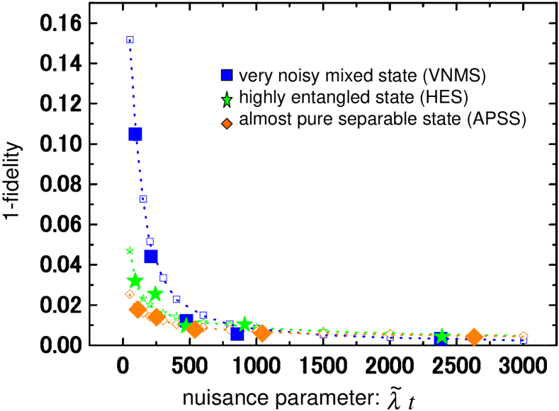
Figure 4: The errors in estimating the three states (the VNMS, the APSS, and the HES) in terms of fidelities between the true states and the estimated states are shown as a function of the nuisanece parameter, $\tilde{\lambda}\,t$ ($\tilde{\lambda}\approx 500$ is coincidence counting rate and $t$ is the data acquisition time of each measurement). The filled plots represent experimental results (the error bars are omitted) and the blank plots represent numerical simulations.

III accuracy of quantum state estimation

Suppose that there are two quantum states, $\rho_{1}$, and $\rho_{2}$; how can the distance between these two quantum states be measured? One possible answer is known as the Bures distance Jozsa1994 ; BC1994 ; Holevo2001 :

$$d_{Bures}(\rho_{1},\rho_{2})^{\,2} = 2(1-\mathop{\mathbf{Tr}}\nolimits[\sqrt{\sqrt{\rho_{1}}\rho_{2}\sqrt{\rho_{1}}}\,])$$ (3)

$$= 2(1-F(\rho_{1},\rho_{2})),$$

where, $F(\rho_{1},\rho_{2})$ is the fidelity. In Sec. II, we have already evaluated the accuracy of the estimation in terms of the fidelities between the true state, $\rho_{\Theta_{0}}$, and the estimated states, $\rho_{\hat{\Theta}}$. We will derive the highest accuracy, which is, in principle, attainable by our tomographic measurements in terms of the Bures distance. Then, it is compared with the experimental results.

Assuming that the estimated states $\rho_{\hat{\Theta}}$ are in the neighborhood of the true state $\rho_{\Theta_{0}}$, the average Bures distance between them can be written as BC1994 ; Holevo2001 ; Uhlmann1993 ; FN1995 ; FujiwaraPhD ; MatsumotoPhD ; Hayashi2002

$$d_{Bures}(\rho_{\Theta_{0}},\rho_{\hat{\Theta}})^{\,2}$$ (4)

$$\approx \!\!\frac{1}{4}\sum_{i=1}^{16}\sum_{j=1}^{16}J_{ij}^{SLD}(\Theta_{0})\,(\hat{\theta}^{i}(N)-\theta_{0}^{i})(\hat{\theta}^{j}(N)-\theta_{0}^{j}),$$

where $\{\theta_{0}^{i}\}_{i=1}^{16}\equiv\{\Theta_{0}\}$ are the true parameters characterizing the true state $\rho_{\Theta_{0}}$ note_Bures , and $\{\hat{\theta}^{i}(N)\}_{i=1}^{16}$ are their estimates inferred from the results of tomographic measurements $\{N\}\equiv\{n_{\nu}\}_{\nu=1}^{16}$; see Appendix A.1 and A.2. Here $[J_{ij}^{SLD}(\Theta)]\equiv\mathop{\mathbf{J}}\nolimits^{SLD}(\Theta)$ is a $16\times 16$ matrix given by the following manner. First, we define a Hermitian operator $\mathop{\mathbf{L}}\nolimits_{i}^{S}(\Theta)$ called symmetric logarithmic derivative (SLD) Holevo2001 ; Helstrom1976 ; Holevo1982 ; ANtext2000 , by

$$\frac{\partial\rho_{\Theta}}{\partial\theta^{i}}=\frac{1}{2}(\mathop{\mathbf{L}}\nolimits_{i}^{S}(\Theta)\,\rho_{\Theta}+\rho_{\Theta}\,\mathop{\mathbf{L}}\nolimits_{i}^{S}(\Theta)).$$ (5)

The SLD $\mathop{\mathbf{L}}\nolimits_{i}^{S}(\Theta)$ can be obtained by solving the equation above and considered as a quantum analogue of the score (classically, the score is defined by $\frac{\partial}{\partial\theta^{i}}\ln[P(N|\Theta)]$ as noted in Appendix A.3). Then the matrix, $\mathop{\mathbf{J}}\nolimits^{SLD}(\Theta)$, called symmetric logarithmic derivative Fisher information matrix (SLD Fisher information matrix), is given by

$$J_{ij}^{SLD}(\Theta)=\frac{1}{2}\mathop{\mathbf{Tr}}\nolimits[\rho_{\Theta}(\mathop{\mathbf{L}}\nolimits_{i}^{S}(\Theta)\mathop{\mathbf{L}}\nolimits_{j}^{S}(\Theta)+\mathop{\mathbf{L}}\nolimits_{j}^{S}(\Theta)\mathop{\mathbf{L}}\nolimits_{i}^{S}(\Theta))].$$ (6)

From Eq. (4), we can see that the Bures distance is locally equivalent to a distance on a Riemannian manifold equipped with a metric structure defined by the SLD Fisher information matrix BC1994 ; Holevo2001 ; Uhlmann1993 ; FN1995 ; FujiwaraPhD ; MatsumotoPhD ; Hayashi2002 . This recognition furnishes us with a geometrical picture of quantum state estimation.

We note here that the SLD Fisher information matrix Eq. (6) was originally introduced for extending classical parameter estimation theory to its quantum counterpart and formulating the quantum Cramér-Rao type lower bound on the errors in estimating quantum states Holevo2001 ; Helstrom1976 ; Holevo1982 ; ANtext2000 ; YL1973 ; BC1994 ; FN1995 ; FujiwaraPhD ; MatsumotoPhD ; Hayashi1998 ; FN1999 ; GM2000 ; Matsumoto2002 .

Our aim here is to evaluate the best accuracy in estimating identically prepared quantum states $\rho_{\Theta_{0}}$ by tomographic measurements. In other words, our aim is to find out the minimum Bures distance between the true states and the estimated states, which can be attained by our tomographic measurements. This can be accomplished by decreasing the value $(\hat{\theta}^{i}(N)-\theta_{0}^{i})(\hat{\theta}^{j}(N)-\theta_{0}^{j})$ of Eq. (4) as much as possible. As is derived in Appendix A.3, the lower bound on the covariance $\mathop{\mathbf{E}}\nolimits_{\Theta_{0}}[(\hat{\theta}^{i}(N)-\theta_{0}^{i})(\hat{\theta}^{j}(N)-\theta_{0}^{j})]$ can be obtained by the Cramér-Rao inequality

$$\mathop{\mathbf{E}}\nolimits_{\Theta_{0}}[(\hat{\theta}^{i}(N)-\theta_{0}^{i})(\hat{\theta}^{j}(N)-\theta_{0}^{j})] \equiv V^{ij}(\Theta_{0})$$ (7)

$$\geq J_{ij}^{\,-1}(\Theta_{0}),$$

where $\mathop{\mathbf{E}}\nolimits_{\Theta_{0}}[f(N)]$ means averaging over the true probability mass function of $\{N\}$ given by Eq. (52) with $\Theta=\Theta_{0}$; $\mathop{\mathbf{J}}\nolimits_{ij}(\Theta_{0})$ is the Fisher information matrix (see Appendix A.3). Since the lower bound on the covariance is known to be asymptotically achievable by using the MLE, the achievable lower bound on the Bures distance can be given by

$$d_{Bures}(\rho_{\Theta_{0}},\rho_{\hat{\Theta}})^{\,2} \approx \frac{1}{4}\sum_{i=1}^{16}\sum_{j=1}^{16}J_{ij}^{SLD}(\Theta_{0})\,V^{ij}(\Theta_{0})$$ (8)

$$\geq \frac{1}{4}\mathop{\mathbf{Tr}}\nolimits[\mathop{\mathbf{J}}\nolimits^{SLD}(\Theta_{0})\,\mathop{\mathbf{J}}\nolimits^{-1}(\Theta_{0}].$$

From Eqs. (45), (52), and (61), the Fisher information matrix $J_{ij}(\Theta_{0})$ can be rewritten as

$$J_{ij}(\Theta_{0})\approx\lambda\bar{J_{ij}}(\Theta_{0})=t\tilde{\lambda}\bar{J_{ij}}(\Theta_{0}),$$ (9)

where

$$\bar{J_{ij}}(\Theta_{0})=-\mathop{\mathbf{E}}\nolimits_{\Theta_{0}}[\frac{\partial^{2}}{\partial\theta^{i}\partial\theta^{j}}\ln[\bar{P}(N|\Theta)]|_{\Theta=\Theta_{0}}],$$ (10)

with

$$\bar{P}(N|\Theta)=\prod_{\nu=1}^{16}e^{-\mathop{\mathbf{Tr}}\nolimits[|m_{\nu}\rangle\langle m_{\nu}|\ \rho_{\Theta}]}\frac{\mathop{\mathbf{Tr}}\nolimits[|m_{\nu}\rangle\langle m_{\nu}|\ \rho_{\Theta}]\,^{n_{\nu}}}{n_{\nu}!}.$$ (11)

Therefore,

$$\mathop{\mathbf{V}}\nolimits(\Theta_{0})\geq\mathop{\mathbf{J}}\nolimits^{-1}(\Theta_{0})=\frac{1}{t\tilde{\lambda}}\bar{\mathop{\mathbf{J}}\nolimits}^{-1}(\Theta_{0}),$$ (12)

that is, in the the asymptotic regime, the errors (the covariance) of the maximum likelihood estimates should be decreasing as inversely proportional to the data acquisition time $t$. Consequently, from Eqs. (3) and (8), we have

$$2(1-F(\rho_{\Theta_{0}},\rho_{\hat{\Theta}}))\geq\frac{1}{4t\tilde{\lambda}}\mathop{\mathbf{Tr}}\nolimits[\mathop{\mathbf{J}}\nolimits^{SLD}(\Theta_{0})\,\bar{\mathop{\mathbf{J}}\nolimits}^{-1}(\Theta_{0})],$$ (13)

or, equivalently,

$$\ln[1-F(\rho_{\Theta_{0}},\rho_{\hat{\Theta}})]$$ (14)

$$\geq -\ln[\lambda]+\ln[\frac{1}{8}\mathop{\mathbf{Tr}}\nolimits[\mathop{\mathbf{J}}\nolimits^{SLD}(\Theta_{0})\,\bar{\mathop{\mathbf{J}}\nolimits}^{-1}(\Theta_{0})]].$$

The logarithm of the average Bures distance between the true state and the estimated state is thus supposed to be decreasing proportional to the logarithm of the nuisance parameter, $\lambda=t\tilde{\lambda}$ (the first term in the right-hand side of Eq. (14)), and all state-dependent properties appear as the intercept on the axis of ordinates (the second term in the right-hand side of Eq. (14)).

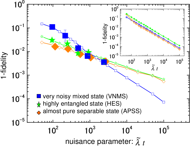
Figure 5: The average Bures distances (divided by 2) between the true states and the states estimated by the MLE are shown as a function of the nuisanece parameter $\tilde{\lambda}\,t$. The filled plots represent experimental results (the vertical error bars correspond to one standard deviation) and the blank plots represent numerical simulations. The inset shows their asymptotic lower bounds.

We note that there are some difficulties for practically calculating the asymptotic lower bound. First, as can be seen in Eq. (60), the calculation of the Fisher information matrix $J_{ij}(\Theta_{0})$ in Eq. (8) includes 16 infinite sum for computing an average over the probability mass function (52). For circumventing this difficulty, we make an approximation;

$$J_{ij}(\Theta_{0})\approx\frac{1}{1000}\sum_{t=1}^{1000}(\frac{\partial}{\partial\theta^{i}}\ln[P(N_{0}^{(t)}|\Theta)]\frac{\partial}{\partial\theta^{j}}\ln[P(N_{0}^{(t)}|\Theta))],$$ (15)

where $\{N_{0}^{(t)}\}$ is numerically simulated (1000 times) according to the Gaussian approximation of $P(N|\Theta_{0})$ in Eq. (52). Second, the inverse of the Fisher information matrix (15) should be derived from the so-called Moore-Penrose generalized inverse MPinverse in case the determinant of the Fisher information matrix becomes zero (the Moore-Penrose generalized inverse provides the unique and well-behaved inverse even for such degenerate matrices). Third, the SLD $\mathop{\mathbf{L}}\nolimits_{i}^{S}(\Theta)$ of Eq. (6) is not uniquely determined from Eq. (5), except for non-degenerate states (the states whose eigenvalues are all non-zero values, that is, the strictly positive states, or the rank-4 states for our specific example). This problem was investigated by Fujiwara, Nagaoka FN1995 , Hayashi Hayashi1998 , and Matsumoto Matsumoto2002 for pure states, and Fujiwara FujiwaraPhD , Matsumoto MatsumotoPhD , and Fujiwara, Nagaoka FN1999 for more general degenerate states. According to their results, any SLDs derived from Eq. (5) results in the same SLD Fisher information matrix $\mathop{\mathbf{J}}\nolimits^{SLD}(\Theta_{0})$. For this reason, we solved Eq. (5) by using the Moore-Penrose generalized inverse, which provides an unique solution for $\mathop{\mathbf{L}}\nolimits_{i}^{S}(\Theta)$ and regarded it as a representative of the SLDs.

To see whether the theoretical predictions, Eq. (14), are truly observed in our experiments, the average Bures distances between the true states and the estimated states as a function of ensemble size, $\tilde{\lambda}\,t$, (i.e., the nuisance parameter) are presented in Fig. 5, where the both axes of Fig. 4 are converted into their logarithms. The calculated asymptotic lower bounds of the average Bures distances are also shown in the inset of Fig. 5. The slight deviation from the linear slope in the small nuisance parameter regime in the inset of Fig. 5, is probably due to the mismatch between the Gaussian approximation used for producing simulated data $\{N_{0}^{(t)}\}$ and their genuine distribution, i.e., Poisson distribution.

In Fig. 5, the average Bures distances clearly depend on what kind of states are to be estimated. However, there are discrepancies between the asymptotic lower bounds (the inset of Fig. (5)) and the experimental results. The discrepancies in the small ensemble region (the left-hand side of Fig. (5)) might be explained by higher order effect of the errors BH1996 (i.e., by the deviations from the first order approximation of the Bures distance in Eq. (4)). On the other hand, the discrepancies in the large ensemble region (the right-hand side of Fig. (5)) cannot be explained by such higher order effects. Except for the results of the VNMS, the expected asymptotic behavior (i.e., the inverse proportionality to the ensemble size) is not observed, even in the results of the numerical simulations. On the other hand, the simulations were carried out including no systematic errors. These facts negate a possibility that the cause of the above discrepancies could stem from perturbations of the experimental condition. Another possibility is that the true state may be slightly biased due to the fact that we determined it by the estimation, thus the (possibly biased) true state plays a major role in the discrepancy. However, for the numerical simulations, this true state is a bona-fide state, which is used as the source to produce the artificial-coincidence-count. This fact nullifies the latter possibility, too.

In the next section, we will elaborate on a possible reason for the discrepancies, and introduce a new estimation strategy based on the Akaike’s information criterion Akaike1974 for reducing the discrepancies and approaching the asymptotic lower bound, Eq. (14).

IV Akaike’s information criterion

Remember that we implicitly assumed that the parametric model of the quantum states (given by Eq. (49) and (50)) is full-rank, that is, we parametrized the quantum states with 16 parameters (including the nuisance parameter); see Appendix A.1 and A.2. However degenerate states, such as the APSS or the HES, might be completely characterized by less than 16 parameters. Subsequently, the surplus parameters give rise to an ambiguity in the numerical procedure of the MLE, i.e., in finding the maximum of the likelihood function, (52). These procedures were executed by FindMinimum, a function of MATHEMATICA 4.0, which is employing the multi-dimensional Powell algorithm, as in Ref. JKMW2001 . However, the minimum found by this function is not necessarily the global minimum. Note that there are some ways to circumvent the problem of such local minimums of likelihood function, e.g., by using the quasi-Newton methods or employing a sophisticated iterative procedures, the expectation-maximization (EM) algorithm followed by unitary transformation, which is due to R̆ehác̆ek et al. RHJ2001 . Here we will, however, give a rather simple but thought-provoking procedure based on the so-called Akaike’s information criterion (AIC) Akaike1974 , which eliminates the redundant parameters.

The AIC is defined by

$$AIC^{(k)}(\Theta)=-2\,\ln[P^{(k)}(N|\Theta)]+2\,k,$$ (16)

where $k$ is the number of independent parameters and $\ln[P^{(k)}(N|\Theta)]$ is the log-likelihood function for the quantum state $\rho_{\Theta}^{(k)}$ which parametrized by $k$ parameters note_AIC . When there are several hypothetical models (with different number of parameters) for estimating a certain state, the model which attains the smallest AIC can be regarded as the most appropriate model because of the following justification. In Appendix A.2, for explaining the MLE, we used the fact that the approximation (54) is valid in the asymptotic region. What Akaike found Akaike1974 is that there is a difference between the mean of the maximum log-likelihood function (right-hand side of (54)) and the maximum log-likelihood function derived by the obtained data (left-hand side of (54)), and the difference can be approximately given by

$$\Delta^{(k)}(\hat{\Theta}) = \frac{1}{t}\ln[P^{(k)}(N|\hat{\Theta})]-\mathop{\mathbf{E}}\nolimits_{\Theta_{0}}[\ln[P^{(k)}(N|\hat{\Theta})]|_{t=1}]$$ (17)

$$\approx \frac{k}{t}.$$

Taking this correction into account, the Kullback-Leibler distance between the true probability mass function $P_{0}(N)$ and its parametric model $P(N|\Theta)$, i.e., Eq. (55), can be minimized by reducing the value,

$$-\mathop{\mathbf{E}}\nolimits_{\Theta_{0}}[\ln[P^{(k)}(N|\hat{\Theta})]|_{t=1}] = -\frac{1}{t}\ln[P^{(k)}(N|\hat{\Theta})]+\frac{k}{t}$$ (18)

$$= \frac{1}{2\,t}AIC^{(k)}(\hat{\Theta}),$$

with respect to the estimators $\{\hat{\Theta}\}$. Therefore, if we choose the model which minimizes the AIC (16) among several alternative parametric models, it is ensured that this model is the closest to the true one from the viewpoint of the Kullback-Leibler distance. The resultant estimate is called minimum AIC estimate (MAICE) Akaike1974 . When a maximum likelihood estimates of a certain model is almost identical to that of another model, the MAICE becomes the one defined with the smaller number of the parameters. The definition of the MAICE gives the mathematical formulation of the principle of parsimony in model selection.

The importance of this new strategy might be more noticeable in estimating quantum states in the infinite-dimensional Hilbert space, e.g., in estimating Wigner function SBRF1993 or density matrix in the number state representation SBPMM1996 . In this situation, somehow vague Fourier-frequency cutoff or truncation of an infinite-dimensional density matrix to finite-dimensional density matrix is introduced in executing the inverse Radon transformation or quantum-state sampling, respectively Leonhardt1997 . We note that Gill and Guţă, recently, made a first attempt addressing this issue GG2003 .

Specifically, for estimating the two qubits, we use

$$\rho_{\Theta}^{(k)}=\frac{T_{\Theta}^{(k)}(T_{\Theta}^{(k)})^{\dagger}}{\mathop{\mathbf{Tr}}\nolimits[T_{\Theta}^{(k)}(T_{\Theta}^{(k)})^{\dagger}]},$$ (19)

where

$$T_{\Theta}^{(16)} = \left[\begin{array}[]{cccc}\theta^{1}&0&0&0\\ \theta^{2}+i\theta^{3}&\theta^{8}&0&0\\ \theta^{4}+i\theta^{5}&\theta^{9}+i\theta^{10}&\theta^{13}&0\\ \theta^{6}+i\theta^{7}&\theta^{11}+i\theta^{12}&\theta^{14}+i\theta^{15}&\theta^{16}\end{array}\right],$$ (24)

$$T_{\Theta}^{(15)} = \left[\begin{array}[]{cccc}\theta^{1}&0&0&0\\ \theta^{2}+i\theta^{3}&\theta^{8}&0&0\\ \theta^{4}+i\theta^{5}&\theta^{9}+i\theta^{10}&\theta^{13}&0\\ \theta^{6}+i\theta^{7}&\theta^{11}+i\theta^{12}&\theta^{14}+i\theta^{15}&0\end{array}\right],$$ (29)

$$T_{\Theta}^{(12)} = \left[\begin{array}[]{cccc}\theta^{1}&0&0&0\\ \theta^{2}+i\theta^{3}&\theta^{8}&0&0\\ \theta^{4}+i\theta^{5}&\theta^{9}+i\theta^{10}&0&0\\ \theta^{6}+i\theta^{7}&\theta^{11}+i\theta^{12}&0&0\end{array}\right],$$ (34)

$$T_{\Theta}^{(7)} = \left[\begin{array}[]{cccc}\theta^{1}&0&0&0\\ \theta^{2}+i\theta^{3}&0&0&0\\ \theta^{4}+i\theta^{5}&0&0&0\\ \theta^{6}+i\theta^{7}&0&0&0\end{array}\right],$$ (39)

thus, $\rho_{\Theta}^{(16)}$, $\rho_{\Theta}^{(15)}$, $\rho_{\Theta}^{(12)}$, and $\rho_{\Theta}^{(7)}$ are representing the rank-4, rank-3, rank-2, and rank-1 density matrices, respectively. Then the AICs are respectively given by

$$AIC^{(16)}(\hat{\Theta}) = -2\,\ln[P^{(16)}(N|\hat{\Theta})]+2\times 16,$$

$$AIC^{(15)}(\hat{\Theta}) = -2\,\ln[P^{(15)}(N|\hat{\Theta})]+2\times 15,$$

$$AIC^{(12)}(\hat{\Theta}) = -2\,\ln[P^{(12)}(N|\hat{\Theta})]+2\times 12,$$

$$AIC^{(7)}(\hat{\Theta}) = -2\,\ln[P^{(7)}(N|\hat{\Theta})]+2\times 7,$$ (40)

where $P^{(k)}(N|\hat{\Theta})$ is the same form of Eq. (52) but replacing $M_{\nu}(\Theta)$ with

$$M^{(k)}_{\nu}(\Theta)=\mathop{\mathbf{Tr}}\nolimits[|m_{\nu}\rangle\langle m_{\nu}|T_{\Theta}^{(k)}(T_{\Theta}^{(k)})^{\dagger}].$$ (41)

Among these models, we can choose the one which minimizes the AIC. As an example, for one of the typical experimental data of coincidence counts for the VNMS (data acquisition time: 5s), $\{N\}$={615, 553, 613, 605, 550, 576, 596, 609, 575, 622, 577, 601, 574, 569, 591, 569}, we have the following AICs; $AIC^{(16)}=163.4$, $AIC^{(15)}=201.3$, $AIC^{(12)}=349.9$ and $AIC^{(7)}=2899.3$. Therefore we choose the rank-4 model $\rho_{\Theta}^{(16)}$. On the other hand, for one of the typical data for the APSS (data acquisition time: 5s), $\{N\}$={42, 45, 25, 2504, 60, 56, 31, 33, 1309, 1431, 1148, 1125, 514, 487, 576, 599}, we have; $AIC^{(16)}=152.8$, $AIC^{(15)}=150.8$, $AIC^{(12)}=146.3$ and $AIC^{(7)}=208.9$. Thus the rank-2 model $\rho_{\Theta}^{(12)}$ is chosen.

It is possible to think about the other hypothetical models, e.g., separable model (which has 7 parameters), or separable and also rank-1 model (which has 5 parameters), but for simplicity, our analyses were confined to the above 4 models.

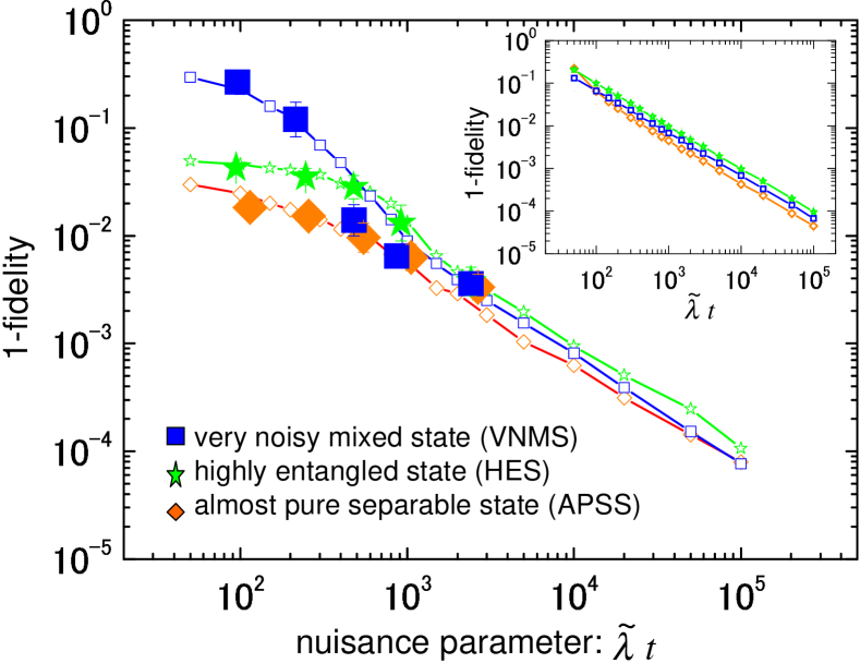
Figure 6: The average Bures distances (divided by 2) between the true states and the MAICEs of the states are shown as a function of the nuisanece parameter $\tilde{\lambda}\,t$. The filled plots represent experimental results (the vertical error bars correspond to one standard deviation) and the blank plots represent numerical simulations. The inset shows their asymptotic lower bounds.

Figure 6 shows the average Bures distances between the true states and the estimated states obtained by employing the new estimation strategy. Their asymptotic lower bounds are also exhibited in the inset of Fig. 6. These asymptotic values were calculated according to Eq. (8). Note that since the true state here was also determined by the MAICE instead of MLE, true state for the APSS and that for the HES resulted in rank-2 density matrices.

As a result of the reduction of the parameters, the MAICEs substantially reduces the discrepancies between the asymptotic lower bounds (the inset) and the experimental results (filled plots: experiments, blank plots: Monte Carlo simulations) comparing to the previous results (Fig. 5). Moreover, in the region where the data acquisition time $t$ greater than 2s, i.e., $\lambda=t\tilde{\lambda}\geq 10^{3}$, the lower bounds of Eq. (13) are almost achieved. This is the case even for estimating degenerate states such as the APSS and the HES. Note also that the intercepts of the asymptotic values on the axis of ordinates shown in the inset of Fig. 6 are slightly lowered comparing to the previous ones (the inset of Fig. 5).

Here we remark that while the numerical simulations continue up to $\lambda=100000$, the maximum data acquisition time of each experiment is 5s, which corresponds to $\lambda\approx 2500$. This is because the systematic errors mentioned above might be getting significant around $\lambda\approx 10000$.

The decreasing rate of the Bures distance for the APSS deviates slightly from the ideal value, -1. This might be due to the residue of the redundant parameters even after making model-inquiry among the above 4 models, because for APSS, the another model (e.g., separable model or separable and rank-1 model) might be more suitable. Thus the further reduction of the parameters might be possible. The discrepancies in small ensemble region (left-hand side of Fig. (6)) may be explained by higher order effect of the errors BH1996 as is mentioned in the previous section.

What kind of factor does dominantly affect the accuracy of the estimation? This question has not been perfectly answered so far. In the general setting of the quantum parameter estimation problem Helstrom1976 ; Holevo1982 ; YL1973 , any kinds of measurements represented as the positive operator-valued measures (POVMs) NCtext2000 are allowed to be utilized. Then not only inseparable projective measurements on the two qubits but even collective measurements on whole ensembles are allowed. In this setting, it has been known that the non-commutativity of quantum mechanics has significant influence on the attainable lower bounds on errors in estimating quantum states with multiple-parameter MatsumotoPhD ; FN1999 . Although significant progress has been made Holevo2001 ; ANtext2000 ; FujiwaraPhD ; MatsumotoPhD ; Hayashi1998 ; FN1999 ; GM2000 ; Matsumoto2002 , finding the asymptotically optimal measurement strategy and obtaining the achievable lower bounds on the errors in estimating quantum states with multiple-parameter are still important open problems.

On the other hand, in our setting, the measurement strategy we employed is not such a optimal collective-measurement strategy, but local tomographic measurements represented by (47). Nonetheless, our results reveal another aspects of the quantum state estimation, that is, the nature of local measurements. Figure 6 shows that the errors in estimating the entangled state, i.e., the HES (which has small entropy but large entanglement; see Fig. 3) is the largest among the three states in the asymptotic region. Thus, the existence of entanglement seems to degrade the accuracy of the estimation if the measurements are performed locally.

V alternative measurement strategy

In this section, we discuss the alternative measurement strategy for two qubits. Since it may be extremely difficult to experimentally realize optimal collective measurements, the following discussion is restricted to projective measurements on just one sample in the ensemble, i.e., on two qubits. Note that there is another favorable measurement strategy, that is, self-learning measurements FKF2000 ; HRBNTW2002 . However, to the best of our knowledge, the lower bound on errors in estimating with this type of adaptive-measurement strategy is still missing.

It is reasonable to expect that if we employ measurements on the inseparable projectors on two qubits, the errors in estimating the entangled states might be reduced. For inspecting whether this expectation is true or not, the following specific projective measurements:

$$\begin{array}[]{c}\frac{1}{2}\,(|HH\rangle+|VV\rangle)(\langle HH|+\langle VV|)\\ \frac{1}{2}\,(|HH\rangle-|VV\rangle)(\langle HH|-\langle VV|)\\ \frac{1}{2}\,(|HV\rangle+|VH\rangle)(\langle HV|+\langle VH|)\\ \frac{1}{2}\,(|HV\rangle-|VH\rangle)(\langle HV|-\langle VH|)\\ \frac{1}{2}\,(|HD\rangle+|VX\rangle)(\langle HD|+\langle VX|)\\ \frac{1}{2}\,(|HD\rangle-|VX\rangle)(\langle HD|-\langle VX|)\\ \frac{1}{2}\,(|HX\rangle+|VD\rangle)(\langle HX|+\langle VD|)\\ \frac{1}{2}\,(|HR\rangle+|VL\rangle)(\langle HR|+\langle VL|)\\ \frac{1}{2}\,(|HR\rangle-|VL\rangle)(\langle HR|-\langle VL|)\\ \frac{1}{2}\,(|HL\rangle+|VR\rangle)(\langle HL|+\langle VR|)\\ |H\rangle\langle H|\otimes\frac{1}{2}I\\ \frac{1}{2}I\otimes|H\rangle\langle H|\\ |D\rangle\langle D|\otimes\frac{1}{2}I\\ \frac{1}{2}I\otimes|D\rangle\langle D|\\ |R\rangle\langle R|\otimes\frac{1}{2}I\\ \frac{1}{2}I\otimes|R\rangle\langle R|,\end{array}$$ (42)

are employed as an alternative to the local tomographic measurements (47). Here, as mentioned in Appendix A.1, $|D\rangle=\frac{1}{\sqrt{2}}(|H\rangle+|V\rangle)$, $|X\rangle=\frac{1}{\sqrt{2}}(|H\rangle-|V\rangle)$, $|R\rangle=\frac{1}{\sqrt{2}}(|H\rangle+i|V\rangle)$, and $|R\rangle=\frac{1}{\sqrt{2}}(|H\rangle-i|V\rangle)$, as $|H\rangle$ and $|V\rangle$ being the horizontal polarization state and vertical one, respectively. This set of 16 projective measurements includes 10 inseparable projectors, and satisfies the condition of tomographic measurements, which is presented in Appendix A.1.

These projective measurements can be realized by slightly modifying the interferometric Bell-state analyzer MMWZ1996 . Figure 7 shows the proposed experimental setup for realizing the projective measurements (42). For 10 inseparable-projective measurements in (42), the down-converted photons are coupled into single mode optical fibers (SMFs) and mixed at 50/50 coupler. Then if the optical path length of two photons are appropriately adjusted and the effects of birefringence in the SMFs are compensated by fiber polarization controller, only two photon whose state of polarization belongs to anti-symmetric subspace, (singlet subspace) contribute the coincidence counts of photon detector (PD) A and B. This coincidence measurement is equivalent to one of the inseparable projective measurements, $\frac{1}{2}\,(|HV\rangle-|VH\rangle)(\langle HV|-\langle VH|)$. The other 9 inseparable measurements can be straightforwardly realized by the local unitary transformation of the state of polarization using half-wave plates (HWP) and quarter-wave plates (QWP) before coupling photons into the SMFs.

For remained 6 local-projective measurements in (42), the state of one-photon polarization is projected on the particular state, e.g., $|H\rangle\langle H|$, by inserting a mirror into the path B (path A) and using HWP, QWP, polarizer, and PD B2 (PD A2 (not shown)) as shown in the dotted box in Fig. 7. Another photon is propagated to either PD A or B. The coincidence measurements of PD B2 (PD A2) and either PD A or PD B are served as the local-projective measurements, e.g., $\frac{1}{2}I\otimes|H\rangle\langle H|$ ($|H\rangle\langle H|\otimes\frac{1}{2}I$).

For utilizing this strategy as an alternative to the local one (47), it is vital to minimize the systematic errors due to imperfect intensity interference in the inseparable measurements. In order to achieve required high visibility of interference, the distinguishability in any degree of freedom of two photons other than the polarization should be reduced. By using SMFs for enhancing spacial-mode overlap of two photons, we expect that such systematic errors due to the spacial degree of freedom might be reduced to some extent. In the recent experiments, the visibilities of this interference exceeding 98% HDFF2002 and even reaching 99.4% PF2003 were reported.

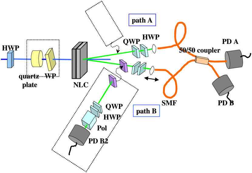
Figure 7: Outline of the proposed experimental setup for realizing the projenctive measurements (42). See text for details.

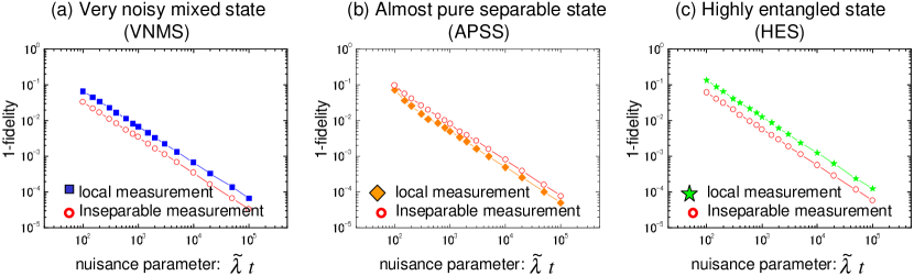
Figure 8: The comparison between the asymptotic lower bounds Eq. (14) for inseparable tomographic measurements (42) and for the conventional local ones (47).

The comparison between the asymptotic lower bounds Eq. (14) for the above inseparable measurements (42) and the conventional local ones (47) is presented in Fig. 8. As expected, the improvement of the accuracy in estimating the HES can be found in Fig. 8 (c), although the accuracy is decreased in estimating the APSS as can be seen in Fig. 8 (b). As indicated in Fig. 8 (a), even for the VNMS, which has no entanglement at all (see Fig. 3), the inseparable measurements (42) are working better than the separable ones (47). This rather surprising result might be viewed as the non-locality without entanglement in quantum state estimation MP1995 ; Hayashi1998 ; GM2000 . We conjecture that for the mixed states like the VNMS, no local tomographic measurements can attain the same accuracy achieved by the inseparable measurements presented in (42). This phenomenon may stem from the fact that the mixed states can be represented as the classical mixture of the entangled states as well as that of the product states.

VI conclusion

We presented quantitative analysis concerning the accuracy of the quantum state estimation, and demonstrated that they depend both on the states to be estimated and on the measurement strategies. For this purpose, the SPDC process was employed for experimentally preparing various ensembles of the bi-photon polarization states and the AIC based new estimation strategy, i.e., the MAICE was introduced for eliminating the numerical problems in the estimation procedures. Our results showed errors of the estimated density matrices decreased as inversely proportional to the ensemble size for all of the three states we examined (the VNMS, the APSS, and the HES) in the asymptotic region. Besides, it was revealed that the existence of entanglement degrade the accuracy of the estimation when the measurements were performed locally on two qubits. The performance of the alternative measurement strategy, which included the projective measurements on inseparable bases, was numerically examined, and we found that the inseparable measurements improved the accuracy in estimating the VNMS as well as the HES.

Further study of the quantum state estimation is sure to pave the way for understanding the ultimate rule for acquiring information from quantum systems.

Appendix A

In Apps. A.1 and A.2, we give a brief review of tomographic measurements and maximum likelihood estimation (MLE), respectively, in accordance with Ref. JKMW2001 . Readers who are familiar with two issues can skip these two Apps. We mention the Cramér-Rao inequality and the Fisher information matrix for providing the optimality of the MLE in Apps. A.3.

A.1 tomographic measurements

With the standard Pauli matrices $\{\sigma_{i}\}_{i=1}^{3}$ supplemented with the identity matrix $\sigma_{0}=I$, an arbitrary density matrix of two qubits can be represented in Hilbert-Schmidt space as a parametric statistical model:

$$\rho_{\Phi}=\sum_{i=0}^{3}\sum_{j=0}^{3}\frac{1}{4}\ (\sigma_{i}\otimes\sigma_{j})\ \phi^{i,j}=\sum_{\mu=0}^{15}\Gamma_{\!\mu}\ \phi^{\mu},$$ (43)

where $\Gamma_{\!4i+j}=\frac{1}{4}\ (\sigma_{i}\otimes\sigma_{j})$ and $\phi^{4i+j}=\phi^{i,j}$. Here $\{\phi^{\mu}\}_{\mu=0}^{15}$ are assumed to be real. From the trace condition of a density matrix, $\phi^{0}$ is equal to one. Note that the above parametric model in Hilbert-Schmidt space does not ensure positivity condition of a density matrix, the problem of positivity is revisited in A.2.

When we try to estimate quantum states as the parametric statistical model of Eq. (43), we should perform some kinds of measurements. Suppose that the measurements are represented by projectors $|m_{\nu}\rangle\langle m_{\nu}|$. Imagining coincidence counting measurements on bi-photon polarization states as a concrete example, the projectors correspond to a certain polarization states. After carrying out the measurements for data acquisition time $t$, the results are given by

$$n_{\nu}=\lambda\mathop{\mathbf{Tr}}\nolimits[|m_{\nu}\rangle\langle m_{\nu}|\rho_{\Phi}],$$ (44)

where

$$\lambda=\tilde{\lambda}\,t,$$ (45)

is the coincidence counts without polarizers for the data acquisition time $t$. Then, $\tilde{\lambda}$ is the coincidence counting rate. Although our attention is focused on the 15 parameters $\{\phi^{\mu}\}_{\mu=0}^{15}$, $\tilde{\lambda}$ is also a priori unknown. Therefore, $\tilde{\lambda}$ is appended to the list of the parameters for estimating the states. The parameter $\lambda$ is thus called the nuisance parameter. Using Eq. (43), Eq. (44) becomes

$$n_{\nu}=\lambda\sum_{\mu=0}^{15}\langle m_{\nu}|\Gamma_{\!\mu}\ |m_{\nu}\rangle\phi^{\mu}=\lambda\sum_{\mu=0}^{15}B_{u\mu}\phi^{\mu}.$$ (46)

Eq. (46) provides a linear relationship between the 16 parameters $\{\phi^{\mu}\}_{\mu=1}^{15}$ and $\lambda$, and the measurement results $\{n_{\nu}\}$. Subsequently, we can derive a necessary and sufficient condition of the measurement for determining these parameters, that is, the matrix $B_{u\mu}$ has an inverse (thus the measurement should consist of at least 16 projectors). Measurements that satisfy the above condition are called tomographic measurements JKMW2001 .

A specific instance of tomographic measurements $\{|m_{u}\rangle\langle m_{u}|\}_{u=1}^{16}$ are note_TM :

$$\begin{array}[]{cccc}|HH\rangle\langle HH|&|HV\rangle\langle HV|&|HD\rangle\langle HD|&|HL\rangle\langle HL|\\ |VH\rangle\langle VH|&|VV\rangle\langle VV|&|VD\rangle\langle VD|&|VL\rangle\langle VL|\\ |DH\rangle\langle DH|&|DV\rangle\langle DV|&|DD\rangle\langle DD|&|DL\rangle\langle DL|\\ |RH\rangle\langle RH|&|RV\rangle\langle RV|&|RD\rangle\langle RD|&|RL\rangle\langle RL|,\end{array}$$ (47)

where $|D\rangle=\frac{1}{\sqrt{2}}(|H\rangle+|V\rangle)$, $|X\rangle=\frac{1}{\sqrt{2}}(|H\rangle-|V\rangle)$, $|R\rangle=\frac{1}{\sqrt{2}}(|H\rangle+i|V\rangle)$, and $|R\rangle=\frac{1}{\sqrt{2}}(|H\rangle-i|V\rangle)$, as $|H\rangle$ and $|V\rangle$ being the horizontal polarization state and vertical one, respectively. Here $|HH\rangle\langle HH|$ means $(|H\rangle\otimes|H\rangle)(\langle H|\otimes\langle H|)$.

From the measurement results $\{n_{\nu}\}_{\nu=1}^{16}\equiv\{N\}$, we can solve linear equation, Eq. (46), with respect to the parameters, $\{\phi^{\mu}\}_{\mu=1}^{15}$ and $\lambda$. As a result, the quantum state of the form Eq. (43) can be uniquely reconstructed. The solutions are explicitly expressed as

$$\phi^{\mu}=\frac{1}{\lambda}\sum_{\nu=1}^{16}[B_{u\mu}]^{-1}n_{\nu}.$$ (48)

This estimation strategy is called the linear tomography JKMW2001 .

A.2 Maximum likelihood estimation

The flaw of the linear tomography in Sec. A.1 is two-fold. One is that there are no considerations about its optimality, another is that the parametric model for linear tomography, Eq. (43), does not ensure the positivity condition of the density matrix as mentioned before. The solution for these flaws is to use maximum likelihood estimation (MLE) JKMW2001 ; BDPS1999 ; RHJ2001 .

Density matrix, which satisfy the positive condition and also the trace condition, can be written as

$$\rho_{\Theta}=\frac{T_{\Theta}T_{\Theta}{}^{\dagger}}{\mathop{\mathbf{Tr}}\nolimits[T_{\Theta}T_{\Theta}{}^{\dagger}]},$$ (49)

where $T_{\Theta}$ is assumed to be a normal matrix. Then, following Ref. JKMW2001 ; BDPS1999 , we adopt the complex lower triangular matrix parametrized by 16 real parameters, $\{\theta^{\mu}\}_{\mu=1}^{16}\equiv\{\Theta\}$, (Cholesky decomposition) as the normal matrix $T_{\Theta}$. It is explicitly written as

$$T_{\Theta}=\left[\begin{array}[]{cccc}\theta^{1}&0&0&0\\ \theta^{2}+i\theta^{3}&\theta^{8}&0&0\\ \theta^{4}+i\theta^{5}&\theta^{9}+i\theta^{10}&\theta^{13}&0\\ \theta^{6}+i\theta^{7}&\theta^{11}+i\theta^{12}&\theta^{14}+i\theta^{15}&\theta^{16}\end{array}\right].$$ (50)

We should keep in mind that while the number of the parameters for the complex lower triangular matrix (50) is 16, that of the density matrix (49) is effectively 15, because of the denominator $\mathop{\mathbf{Tr}}\nolimits[T_{\Theta}T_{\Theta}{}^{\dagger}]$.

The coincidence counts $\{N\}=\{n_{\nu}\}_{\nu=1}^{16}$ are assumed to obey the Poisson distribution with the mean being

$$M_{\nu}(\Theta) \equiv \lambda\mathop{\mathbf{Tr}}\nolimits[|m_{\nu}\rangle\langle m_{\nu}|\rho_{\Theta}]$$ (51)

$$= \mathop{\mathbf{Tr}}\nolimits[|m_{\nu}\rangle\langle m_{\nu}|T_{\Theta}T_{\Theta}{}^{\dagger}],$$

where we rearrange the parameters in Eq. (50) so that the value of $\mathop{\mathbf{Tr}}\nolimits[T_{\Theta}T_{\Theta}{}^{\dagger}]$ coincides with the nuisance parameter $\lambda$ of Eq. (45). Thus the probability mass function (Poisson density function) of the measurement results $\{N\}$ for given values of the parameters $\{\Theta\}$ is written as

$$P(N|\Theta)=\prod_{\nu=1}^{16}e^{-M_{\nu}(\Theta)}\frac{M_{\nu}(\Theta)\,^{n_{\nu}}}{n_{\nu}!}\equiv\prod_{\nu=1}^{16}p(n_{\nu}|\Theta).$$ (52)

Although the parametric model, Eq. (49), guarantees the positivity and trace condition, the simple linear relationship between the results of measurements $\{N\}$ and the parameters $\{\Theta\}$ like Eq. (46) has disappeared. Nonetheless, the MLE can be applied for inferring the parameters $\{\Theta\}$ from the observed results $\{n_{\nu}\}_{\nu=1}^{16}=\{N\}$ note_condition . We can regard Eq. (52) as a function on the 16-dimensional parameter space where each point corresponds to a certain quantum state. It is called likelihood function. Then, it is reasonable to consider that the point (state) which maximizes the likelihood function (52) is likely to be the nearest to the true point (state), $\{\theta_{0}^{1},\theta_{0}^{2},\ldots,\theta_{0}^{16}\}\equiv\{\Theta_{0}\}$. The strategy to choose the values $\{\hat{\theta^{1}}(N),\hat{\theta^{2}}(N),\ldots,\hat{\theta^{16}}(N)\}$ which maximizes Eq. (52) as the estimates is called maximum likelihood estimation (MLE).

The MLE is elucidated based on the Kullback-Leibler distance (relative entropy) NCtext2000 ; CTtext1991 ; ANtext2000 . It is often convenient to consider the natural logarithm of the likelihood function $P(N|\Theta)$, which is called log-likelihood function:

$$\ln[P(N|\Theta)]=\sum_{\nu=1}^{16}\ln[p(n_{\nu}|\Theta)].$$ (53)

Here it is apparent that this change does not influence the location of the maximum. As the data acquisition time $t$ is increased infinitely, the log-likelihood function divided by $t$ tends, with probability 1, to the the mean log-likelihood function for unit time, $t=1$, i.e.,

$$\frac{1}{t}\ln[P(N|\Theta)] \approx \!\!\sum_{n_{1}=0}^{\infty}\sum_{n_{2}=0}^{\infty}\cdots\!\!\sum_{n_{16}=0}^{\infty}\!\!P_{0}(N)\ln[P(N|\Theta)]|_{t=1}$$ (54)

$$\equiv\mathop{\mathbf{E}}\nolimits_{\Theta_{0}}[\ln[P(N|\Theta)]|_{t=1}],$$

where $P_{0}(N)\equiv P(N|\Theta_{0})$ is the true probability mass function of $\{N\}$. The difference between the true probability mass function $P_{0}(N)$ and the parametric model $P(N|\Theta)$ can be measured by the Kullback-Leibler distance NCtext2000 ; CTtext1991 ; ANtext2000 ,

$$D(P_{0}(N)\,\|\,P(N|\Theta))=\mathop{\mathbf{E}}\nolimits_{\Theta_{0}}[\ln[P_{0}(N)]-\ln[P(N|\Theta)]].$$ (55)

This takes a positive value, unless $P_{0}(N)=P(N|\Theta)$ in all $\{N\}$ (in this case $D(P_{0}(N)\,\|\,P(N|\Theta))=0$). Then it becomes clear that what we try to do by the MLE (i.e., to increase the log-likelihood function, Eq. (54), with respect to $\{\Theta\}$) is to minimize the Kullback-Leibler distance between the true probability mass function $P_{0}(N)$ and its parametric model $P(N|\Theta)$.

A.3 Cramér-Rao bound and
Fisher information matrix

The MLE is supposed to be the optimal estimation strategy in the following sense. The errors of the estimates $\{\hat{\theta^{1}}(N),\hat{\theta^{2}}(N),\ldots,\hat{\theta^{16}}(N)\}=\{\hat{\Theta}(N)\}$ can be represented by the covariance matrix $\mathop{\mathbf{V}}\nolimits(\Theta_{0})=[V^{ij}(\Theta_{0})]$ which is given by

$$V^{ij}(\Theta_{0})$$

$$= \mathop{\mathbf{E}}\nolimits_{\Theta_{0}}[(\hat{\theta^{i}}(N)\!-\!\mathop{\mathbf{E}}\nolimits_{\Theta_{0}}[\hat{\theta^{i}}(N)])(\hat{\theta^{j}}(N)\!-\!\mathop{\mathbf{E}}\nolimits_{\Theta_{0}}[\hat{\theta^{j}}(N)])].$$

The Cramér-Rao inequality provides an asymptotic lower bound on the covariance matrix $\mathop{\mathbf{V}}\nolimits(\Theta_{0})$ as follows Helstrom1976 ; CTtext1991 ; ANtext2000 . We first assume the unbiasedness of the estimates $\hat{\theta^{i}}(N)$, i.e.,

$$\mathop{\mathbf{E}}\nolimits_{\Theta_{0}}[(\hat{\theta^{i}}(N)-\theta_{0}^{\,i})]=0.$$ (57)

Then we define the score of the probability mass function as

$$S_{i}(N|\Theta_{0})\equiv\frac{\partial}{\partial\theta^{i}}\ln[P(N|\Theta)]|_{\Theta=\Theta_{0}}=\frac{\frac{\partial}{\partial\theta^{i}}P(N|\Theta)|_{\Theta=\Theta_{0}}}{P(N|\Theta_{0})}.$$ (58)

Here, we can readily verify the mean of the score is zero, i.e.,

$$\mathop{\mathbf{E}}\nolimits_{\Theta_{0}}[S_{i}(N|\Theta_{0})]=0.$$ (59)

Thus, the covariance of the score can be written as

$$J_{ij}(\Theta_{0})=\mathop{\mathbf{E}}\nolimits_{\Theta_{0}}[S_{i}(N|\Theta_{0})S_{j}(N|\Theta_{0})].$$ (60)

Equivalently, we have

$$J_{ij}(\Theta_{0})=-\mathop{\mathbf{E}}\nolimits_{\Theta_{0}}[\frac{\partial^{2}}{\partial\theta^{i}\partial\theta^{j}}\ln[P(N|\Theta)]|_{\Theta=\Theta_{0}}],$$ (61)

as can be seen from differentiating Eq. (59) with respect to $\theta^{j}$. The covariance matrix of the score, $\mathop{\mathbf{J}}\nolimits(\Theta_{0})\equiv[J_{ij}(\Theta_{0})]$, is well known as the Fisher information matrix. By the Schwarz inequality for expectation, we have

$$(\mathop{\mathbf{E}}\nolimits_{\Theta_{0}}[\sum_{i=1}^{16}z_{i}S_{i}(N|\Theta_{0})\,\sum_{j=1}^{16}y_{j}(\hat{\theta^{j}}(N)-\theta_{0}^{\,j})])^{2}$$ (62)

$${\leq} [\sum_{i=1}^{16}\sum_{j=1}^{16}z_{i}z_{j}J_{ij}(\Theta_{0})][\sum_{i=1}^{16}\sum_{j=1}^{16}y_{i}y_{j}V^{ij}(\Theta_{0})].$$

where, we introduce two sets of 16 auxiliary real variables $(y_{1},y_{2},\ldots,y_{16})\equiv\,^{t}\!\mathop{\mathbf{y}}\nolimits$ and $(z_{1},z_{2},\ldots,z_{16})\equiv\,^{t}\!\mathop{\mathbf{z}}\nolimits$. From Eq. (59), we have

$$\mathop{\mathbf{E}}\nolimits_{\Theta_{0}}[S_{i}(N|\Theta_{0})\,(\hat{\theta^{j}}(N)-\theta_{0}^{\,j})]$$ (63)

$$= \mathop{\mathbf{E}}\nolimits_{\Theta_{0}}[S_{i}(N|\Theta_{0})\,\hat{\theta^{j}}(N)]$$

$$= \!\!\sum_{n_{1}=0}^{\infty}\sum_{n_{2}=0}^{\infty}\cdots\sum_{n_{16}=0}^{\infty}\!\!P(N|\Theta_{0})\frac{\frac{\partial}{\partial\theta^{i}}P(N|\Theta)|_{\Theta=\Theta_{0}}}{P(N|\Theta_{0})}\hat{\theta^{j}}(N)$$

$$= \frac{\partial}{\partial\theta^{i}}\sum_{n_{1}=0}^{\infty}\sum_{n_{2}=0}^{\infty}\cdots\sum_{n_{16}=0}^{\infty}\!\!P(N|\Theta)\hat{\theta^{j}}(N)|_{\Theta=\Theta_{0}}$$

$$= \delta^{j}_{i},$$

where $\delta^{j}_{i}$ is the Kronecker’s delta. Consequently, the left-hand side of the inequality (62) becomes

$$(\sum_{i=1}^{16}\sum_{i=1}^{16}z_{i}y_{j}\delta^{j}_{i})^{2}=(\,^{t}\!\mathop{\mathbf{y}}\nolimits\mathop{\mathbf{z}}\nolimits)^{2}.$$ (64)

By substituting Eq. (64) and putting $\mathop{\mathbf{z}}\nolimits=\mathop{\mathbf{J}}\nolimits(\Theta_{0})^{-1}\mathop{\mathbf{y}}\nolimits$ in the Schwarz inequality (62), we obtain

$$\,{}^{t}\!\mathop{\mathbf{y}}\nolimits\mathop{\mathbf{J}}\nolimits(\Theta_{0})^{-1}\mathop{\mathbf{y}}\nolimits\leq\,^{t}\!\mathop{\mathbf{y}}\nolimits\mathop{\mathbf{V}}\nolimits(\Theta_{0})\mathop{\mathbf{y}}\nolimits,$$ (65)

that is,

$$\mathop{\mathbf{V}}\nolimits(\Theta_{0})\geq\mathop{\mathbf{J}}\nolimits^{-1}(\Theta_{0}),$$ (66)

which is the Cramér-Rao inequality for unbiased estimates. Note that most estimators used in practice are not unbiased. However, the Cramér-Rao bound on the variance of an unbiased estimator is asymptotically also a bound on the mean square error,

$$\mathcal{V}^{ij}(\Theta_{0})=\mathop{\mathbf{E}}\nolimits_{\Theta_{0}}[(\hat{\theta^{i}}(N)-\theta_{0}^{i})(\hat{\theta^{j}}(N)-\theta_{0}^{j})].$$ (67)

of any well-behaved estimator, as shown by Gill and Massar in Ref. GM2000 . Thus, the Cramér-Rao inequality provides us with an asymptotic lower bound on the covariance matrix $\mathop{\mathbf{V}}\nolimits(\Theta_{0})$ for wide variety of estimates in terms of the Fisher information matrix Helstrom1976 ; GM2000 ; CTtext1991 ; ANtext2000 . Here, we mention the significant fact that the maximum likelihood estimates are asymptotically efficient, in other words, by the MLE, the covariance matrix asymptotically achieves the Cramér-Rao lower bound ANtext2000 ; Braunstein1992 . In this sense, the MLE is the optimal strategy.

References

- (1) S. Massar and S. Popescu, Phys. Rev. Lett. 74, 1259 (1995).
- (2) M. A. Nielsen and I. L. Chuang, Quantum Computation and Quantum Information (Cambridge University Press, Cambridge, 2000).
- (3) U. Leonhardt, Measuring the Quantum State of Light (Cambridge University Press, Cambridge, 1997).
- (4) D. T. Smithey, M. Beck, M. G. Raymer and A. Faridani, Phys. Rev. Lett. 70, 1244 (1993)
- (5) S. Schiller, G. Breitenbach, S. F. Pereira, T. Müller, and J. Mlynek, Phys. Rev. Lett. 77, 2933 (1996)
- (6) A. I. Lvovsky, H. Hansen, T. Aichele, O. Benson, J. Mlynek, and S. Schiller, Phys. Rev. Lett. 87, 050402 (2001)
- (7) P. Bertet, A. Auffeves, P. Maioli, S. Osnaghi, T. Meunier, M. Brune, J. M. Raimond, and S. Haroche, Phys. Rev. Lett. 89, 200402 (2002)
- (8) A. G. White, D. F. V. James, P. H. Eberhard, and P. G. Kwiat, Phys. Rev. Lett. 83 3103 (1999).
- (9) P. G. Kwiat, A. J. Berglund, J. B. Altepeter, and A. G. White, Science 290 498 (2000).
- (10) P. G. Kwiat, S. Barraza-Lopez, A. Stefanov, and N. Gisin, Nature (London) 409 1014 (2001).
- (11) M. Xiao, L. -A. Wu, and H. J. Kimble, Phys. Rev. Lett. 59, 278 (1987); Y. -Q. Li, D. Guzun, and M. Xiao, Phys. Rev. Lett. 82, 5225 (1999); M. A. Armen, J. K. Au, J. K. Stockton, A. C. Doherty, and H. Mabuchi, Phys. Rev. Lett. 89, 133602 (2002)
- (12) P. Grangier, R. E. Slusher, B. Yurke, and A. LaPorta, Phys. Rev. Lett. 59, 2153 (1987); A. Kuzmich and L. Mandel, Quantum Semiclass. Opt. 10, 493 (1998); G. Santarelli, Ph. Laurent, P. Lemonde, A. Clairon, A. G. Mann, S. Chang, A. N. Luiten, and C. Salomon, Phys. Rev. Lett. 82, 4619 (1999).
- (13) S. J. Freedman and J. F. Clauser, Phys. Rev. Lett. 28, 938 (1972); A. Aspect, J. Dalibard, and G. Roger, Phys. Rev. Lett. 49, 1804 (1982); G. Weihs, T. Jennewein, C. Simon, H. Weinfurter, and A. Zeilinger, Phys. Rev. Lett. 81, 5039 (1998).
- (14) D. Bouwmeester, J. -W. Pan, K. Mattle, M. Eibl, H. Weinfurter, and A. Zeilinger, Nature (London) 390 575 (1997).
- (15) T. Jennewein, C. Simon, G. Weihs, H. Weinfurter, and A. Zeilinger, Phys. Rev. Lett. 84, 4729 (2000); D. S. Naik, C. G. Peterson, A. G. White, A. J. Berglund, and P. G. Kwiat, Phys. Rev. Lett. 84, 4733 (2000); W. Tittel, J. Brendel, H. Zbinden, and N. Gisin Phys. Rev. Lett. 84, 4737 (2000).
- (16) P. G. Kwiat, E. Waks, A. G. White, I. Appelbaum, and P. H. Eberhard, Phys. Rev. A 60 R773 (1999).
- (17) D. F. V. James, P. G. Kwiat, W. J. Munro, and A. G. White, Phys. Rev. A 64 052312 (2001).
- (18) A. G. White, D. F. V. James, W. J. Munro, and P. G. Kwiat, Phys. Rev. A 65 012301 (2001).
- (19) Y. Nambu, K. Usami, Y. Tsuda, K. Matsumoto, and K. Nakamura, Phys. Rev. A 66 033816 (2002).
- (20) H. Akaike, IEEE trans. Automat.Contr 19 716 (1974).
- (21) K. Banaszek, G. M. D’Ariano, M. G. A. Paris, and M. F. Sacchi, Phys. Rev. A 61 010304(R) (1999).
- (22) J. R̆ehác̆ek, Z. Hradil, and M. Jez̆ek, Phys. Rev. A 63 040303(R) (2001).
- (23) R. Jozsa, J. Mod. Opt. 41, 2315 (1994).
- (24) H. Barnum, C. M. Caves, C. A. Fuchs, R. Jozsa, and B. Schumacher Phys. Rev. Lett. 76 2818 (1996).
- (25) S. L. Braunstein and C. M. Caves, Phys. Rev. Lett. 72 3439 (1994).
- (26) A. S. Holevo, Statistical Structure of Quantum Theory (Springer, Heidelberg, 2001).
- (27) A. Uhlmann, Rep. Math. Phys. 33, 253 (1993).
- (28) A. Fujiwara and H. Nagaoka, Phys. Lett. A 201 119 (1995).
- (29) A. Fujiwara, A geometrical study in quantum information systems, Ph.D. Thesis, The University of Tokyo (1995).
- (30) K. Matsumoto, A geometrical approach to quantum estimation theory, Ph.D. Thesis, The University of Tokyo (1997).
- (31) M. Hayashi, quant-ph/0202003.
- (32) The Bures distance does not depend on parametrization. Therefore we can use any parametrization.
- (33) C. W. Helstrom, Quantum Detection and Estimation Theory (Academic Press, New York, 1976).
- (34) A. S. Holevo, Probabilistic and Statistical Aspects of Quantum Theory (North-Holland, Amsterdam, 1982).
- (35) S. Amari and H. Nagaoka, Methods of Information Geometry (AMS, Providence, 2000).
- (36) H. P. Yuen and M. Lax, IEEE trans. Inf. Theory 19, 740 (1973)
- (37) M. Hayashi, J. Phys. A: Math. Gen. 30, 4633 (1998).
- (38) A. Fujiwara and H. Nagaoka, J. Math. Phys. 40, 4227 (1999).
- (39) R. D. Gill and S. Massar, Phys. Rev. A 61 042312 (2000).
- (40) K. Matsumoto, J. Phys. A: Math. Gen. 35, 3111 (2002).
- (41) MATHEMATICA 4.0 has a function, PseudoInverse, by which we can calculate the Moore-Penrose generalized inverse of degenerate matrices.
- (42) D. C. Brody and L. P. Hughston, Phys. Rev. Lett. 77 2851 (1996).
- (43) The factor 2 of AIC is not important but a remnant of the original form Akaike1974 .
- (44) R. Gill and M. I. Guţă, quant-ph/0303020.
- (45) D. G. Fischer, S. H. Kienle, and M. Freyberger, Phys. Rev. A 61 032306 (2000).
- (46) Th. Hannemann, D. Reiss, Ch. Balzer, W. Neuhauser, P. E. Toschek, and Ch. Wunderlich, Phys. Rev. A 65 050303 (2002).
- (47) M. Michler, K. Mattle, H. Weinfurter, and A. Zeilinger, Phys. Rev. A 53 R1209 (1996).
- (48) M. Hendrych, M. Dus̆ek, R. Filip, and J. Fiurás̆ek, quant-ph/0208091.
- (49) T. B. Pittman and J. D. Franson, quant-ph/0301169.
- (50) This set of the projectors is slightly different from that of Ref. WJEK1999 ; JKMW2001 .
- (51) A necessary and the sufficient condition of tomographic measurements for the linear tomography is not straightforwardly applied to that for the MLE; nonetheless, we use these condition, because of its simplicity and the fact that it is at least valid as the sufficient condition for inferring the parameters by the MLE.
- (52) T. Cover and J. Thomas, Elements of Information Theory (Wiley, New York, 1991).
- (53) S. L. Braunstein, J. Phys. A: Math. Gen. 25, 3813 (1992).