Beam Splitter Entangler for Light Fields

Abstract

We propose an experimentally feasible scheme to generate various types of entangled states of light fields by using beam splitters and single-photon detectors. Two light fields are incident on two beam splitters and are split into strong and weak output modes respectively. A conditional joint measurement on both weak output modes may result in an entanglement between the two strong output modes. The conditions for the maximal entanglement are discussed based on the concurrence. Several specific examples are also examined.

Quantum entanglement has been identified as a basic resource in achieving tasks of quantum communication and quantum computation 1 . Photons are considered to be the best quantum information carriers over long distances, and those in entangled states have been used to experimentally demonstrate quantum teleportation 2 , quantum dense coding 3 , quantum cryptography 4 , and the generation of GHZ-states of three or four photons 5 .

In comparison with other candidates for engineering quantum entanglement, light fields possess more abundant capacity to create various types of entangled states including the discrete, the continuous variable, and the combination of the both. Almost all of the reported experiments adopted the parametric down-conversion process as a standard source for the entangled photon pairs as well as two-mode squeezed states. Recently it was found that linear optical elements, such as beam-splitters and polarization beam-splitters, can also be used to generate entangled light fields 6 ; 7 ; 8 ; 9 ; 10 ; 11 . In Ref. 6 , an efficient quantum computation with linear optics is devised, it is undoubtedly an entangler for light fields. On the other hand, a single beam splitter can also act as an entangler for light fields if the input modes are in appropriate nonclassical states 10 ; 11 . However, the types of the resultant entangled states from the existent schemes are still very limited and cannot satisfy the requirements for quantum information processing and for other applications. Thus how to generate various types of entangled states of light fields is still of great significance.

Very recently several schemes have been proposed to entangle distant atoms 12 and atomic ensembles 13 by means of photon interference. It is natural to ask whether the idea of photon interference can be extended to the generation of the entangled states of light fields. This letter will give a positive answer.

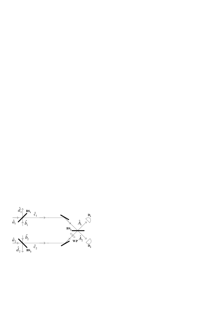
Figure 1: Experimental setup. Two input light fields in modes $\hat{b}_{1}$ and $\hat{b}_{2}$ are incident on BS₁ and BS${}_{2},$ and split into weak outputs in modes $\hat{c}_{1}$ and $\hat{c}_{2}$ and strong outputs in modes $\hat{d}_{1}$ and $\hat{d}_{2}$. Photons in weak outputs are then mixed on BS₃ and subsequently detected by single-photon detectors D₁ and D₂.

In this letter we present an experimentally feasible scheme for the generation of entangled states of light fields by using beam splitters and the single-photon detectors. The setup we are considering here consists of three lossless beam splitters, BS₁, BS₂ and BS₃, and two single-photon detectors D₁ and D₂, as shown in Fig. 1. For simplicity, we assume that BS₁ and BS₂ are of the same amplitude reflection and transmission coefficients $R$ and $T$ with a relation $|R|^{2}+|T|^{2}=1,$ and that the distance from BS₁ to BS₃ is the same as that from BS₂ to BS₃. As an optical element, a beam splitter generally has two input ports and two output ports. In our setup only one input port has a non-zero input field for both BS₁ and BS₂, the other input port is always left in the vacuum state. In this case the non-zero input field will be split into two output fields. As has been proved, the two output fields may be entangled when the input field is in an appropriate nonclassical state 10 ; 11 . The entanglement quantity and the properties of the output fields depend to a large extent on the input fields as well as on the amplitude reflection and transmission coefficients $R$ and $T$ of the beam splitter. If $R$ and $T$ of the beam splitter BS₁ (and BS₂) are largely different, the non-zero input field will be split into two output fields in which one is very strong, and the other is very weak. In fact, we can design BS₁ and BS₂ in such a way that the weak output field possesses maximally one photon, that is, the weak output mode is in the vacuum state $|0\rangle$ or in the one photon number state $|1\rangle.$ Correspondingly the strong output mode will be in a state that keeps the photon number of the input field unchanged or in a state that annihilates one photon from the input field since the lossless beam splitter conserves the photon number of the input fields. In this way we have prepared a specific entangled state of the weak and the strong output fields. Subsequently we let the two weak output fields from BS₁ and BS₂ be combined at BS₃, a 50%:50% beam splitter, and then detected by single-photon detectors D₁ and D₂. If only one photon is registered by D₁ or D₂, we successfully generate an entangled state of the two strong output fields of BS₁ and BS₂. Otherwise, we fail to generate the desired entangled state and should repeat the process again until one photon is registered.

Our scheme is based on a simple optical element, the beam splitter. The perfection of the beam splitter is very high, the requirements for BS₁ and BS₂ can thus be satisfied with the required precision easily, therefore our scheme is experimentally feasible. In particular, as will be shown below, our scheme can be used to generate various types of entangled states of light fields.

In order to illustrate our method explicitly, we first examine the effect of a beam splitter on its output fields. Let us denote by $\hat{a}_{j},\hat{b}_{j}$ the input mode amplitudes shown in Fig. 1 and by $\hat{c}_{j},\hat{d}_{j}$ the output mode amplitudes, where the subscript $j$ stands for BS_j($j=1,2$). Suppose the initial quantum state of the input fields for BS_j is a product state, $|0,\psi_{j}\rangle_{in}=|0\rangle_{a_{j}}\otimes|\psi_{i}\rangle_{b_{j}}$, in which the mode $\hat{a}_{j}$ is supposed to be always in the vacuum state $|0\rangle_{a_{j}}$ and the mode $\hat{b}_{j}$ in a superposition of the photon number states which can be expressed as

$$|\psi_{j}\rangle=\sum_{n=0}^{\infty}f_{n}^{(j)}|n\rangle,$$ (1)

with the normalized condition $\sum_{n=0}^{\infty}|f_{n}^{(j)}|^{2}=1$. The output fields are then of the following form 14 ,

where the beam splitter operator is

$$\hat{B}_{j}=\exp\left[{\frac{\theta}{2}}(\hat{a}_{j}^{{\dagger}}\hat{b}_{j}e^{i\phi}-\hat{a}_{j}\hat{b}_{j}^{{\dagger}}e^{-i\phi})\right],$$ (3)

with the amplitude reflection and transmission coefficients $T=\cos{\frac{\theta}{2}},~{}~{}R=\sin{\frac{\theta}{2}}$. Here $\phi$ denotes the phase difference between the reflected and transmitted fields.

The terms $\hat{B}_{j}|0,n\rangle_{in}$ in Eq. (2) can be evaluated according to Eq. (3),

$$\hat{B}|0,n\rangle_{in}=\sum_{k=0}^{n}c_{k}^{n}|k,n-k\rangle_{out},$$ (4)

where $|k,n-k\rangle_{out}=|k\rangle_{c}\otimes|n-k\rangle_{d}$, and $c_{k}^{n}=\binom{n}{k}^{1/2}\exp\left(ik\phi\right)R^{k}T^{n-k}.$

In the following we assume that the amplitude reflection coefficient $R$ for BS_j ($j=1,2$) is so small ($R\ll T$) that the terms containing $R^{k}$ in Eq. (4) can be neglected when $k\geqslant 2$, thus Eq. (4) is simplified as

$$\hat{B}_{j}|0,n\rangle_{in}$$ (2)

$$\approx T^{n}|0,n\rangle_{out}+\exp\left(i\phi\right)RT^{n-1}\sqrt{n}|1,n-1\rangle_{out}$$

$$= T^{n}|0,n\rangle_{out}+\exp\left(i\phi\right)RT^{n-1}\hat{d}_{j}|1,n\rangle_{out}.\TCItag{5}$$

Substituting Eq. (5) into Eq. (2) we get

$$|\Psi_{j}\rangle_{out}=|0\rangle_{c_{j}}\otimes|u_{j}\rangle_{d_{j}}+\exp\left(i\phi\right)R|1\rangle_{c_{j}}\otimes|v_{j}\rangle_{d_{j}},$$ (6)

where $|u_{j}\rangle$ and $|v_{j}\rangle$ take the form

$$|u_{j}\rangle = \sum_{n=0}^{\infty}f_{n}^{(j)}T^{n}|n\rangle,\TCItag{7a}$$ (3)

$$|v_{j}\rangle = \hat{d}_{j}\sum_{n=0}^{\infty}f_{n+1}^{(j)}T^{n}|n+1\rangle.\TCItag{7b}$$ (4)

The state (6) is a specific entangled state in which the mode $\hat{c}_{j}$ (i.e. the weak mode) possesses maximally one photon.

Now we show how to generate the entangled states of two strong output modes $\hat{d}_{1}$ and $\hat{d}_{2}$ by manipulating the two weak modes $\hat{c}_{1}$ and $\hat{c}_{2}$. As shown in Fig. 1, we suppose the two input fields are, respectively, incident on BS₁ and BS₂ simultaneously. Afterwards the two weak output modes $\hat{c}_{1}$ and $\hat{c}_{2}$ are combined at BS₃ with the output mode amplitudes $\hat{A}_{1}=\left[i\hat{c}_{1}+e^{i\gamma}\hat{c}_{2}\right]/\sqrt{2}$,$~{}\hat{A}_{2}=\left[\hat{c}_{1}+ie^{i\gamma}\hat{c}_{2}\right]/\sqrt{2}$. Here the factor $i$ denotes a $\pi/2$ phase shift between the reflected and the transmitted modes, and $\gamma$ denotes the phase shift induced by a wave plate (WP) placed in the path of mode $\hat{c}_{2}$. The detection of a single photon by D₁ or D₂ is accompanied by the wave function collapse $|\Psi_{1}\rangle_{out}\otimes|\Psi_{2}\rangle_{out}\rightarrow\hat{A}_{1,2}(|\Psi_{1}\rangle_{out}\otimes|\Psi_{2}\rangle_{out})$. Neglecting the high-order terms $o(R^{2}),$ we find the final state of the two strong modes, conditional on a click of either D₁ or D₂, takes the following form,

$$|\Phi\rangle_{1,2}=|v_{1}\rangle|u_{2}\rangle\mp i\exp\left(i\gamma\right)|u_{1}\rangle|v_{2}\rangle.$$ (8)

Here and in what follows the subscripts $d_{j}$ are omitted to simplify the notation. Note that the state (8) is not normalized. The probability for successfully generating the above state is proportional to $R^{2}$. The phase factor in state (8) can be controlled through the WP.

In principle, the scheme we proposed here is closely related to the quantum entanglement swapping 15 in which the particles that have never interacted directly are entangled, and can be regarded as a specific version of entanglement concentration protocol by using entanglement swapping 16 . The entanglement between the weak and the strong output fields for both BS₁ and BS₂ is a necessary condition for the successful generation of the desired entangled state (8). Accordingly the requirement that both input fields of BS₁ and BS₂ are in nonclassical states should be satisfied 10 ; 11 .

Now let us examine the entanglement properties of the resultant state (8). To this end, we first transform it to the normalized basis,

$$|\Phi\rangle_{1,2}=\nu_{1}\mu_{2}|V_{1}\rangle|U_{2}\rangle\mp i\exp\left(i\gamma\right)\mu_{1}\nu_{2}|U_{1}\rangle|V_{2}\rangle,$$ (9)

where $|U_{j}\rangle=|u_{j}\rangle/\mu_{j}$, $|V_{j}\rangle=|v_{j}\rangle/\nu_{j}$ are normalized states for system $j$ with the normalized constants

$$\mu_{j} = \left(\sum_{n=0}^{\infty}|T^{n}f_{n}^{(j)}|^{2}\right)^{\frac{1}{2}},\TCItag{10a}$$ (5)

$$\nu_{j} = \left(\sum_{n=0}^{\infty}\left(n+1\right)|T^{n}f_{n+1}^{(j)}|^{2}\right)^{\frac{1}{2}}.\TCItag{10b}$$ (6)

Considering $|U_{j}\rangle$ and $|V_{j}\rangle$ may be nonorthogonal, the state (9) is actually a general bipartite entangled state. The concurrence 17 has been proved to be a convenient entanglement measure for such states and has been evaluated by Wang 18 . We find the concurrence of the entangled state (9) takes the form

$$C_{1,2}=\frac{2\mu_{1}\nu_{1}\mu_{2}\nu_{2}\sqrt{\left(1-|\langle V_{1}|U_{1}\rangle|^{2}\right)\left(1-|\langle V_{2}|U_{2}\rangle|^{2}\right)}}{\mu_{1}^{2}\nu_{2}^{2}+\nu_{1}^{2}\mu_{2}^{2}+\mu_{1}\nu_{1}\mu_{2}\nu_{2}\left(\pm i\text{e}^{-i\gamma}\langle U_{1}|V_{1}\rangle\langle V_{2}|U_{2}\rangle\mp i\text{e}^{i\gamma}\langle V_{1}|U_{1}\rangle\langle U_{2}|V_{2}\rangle\right)}.$$ (11)

The concurrence ranges from 0 to 1 with the value 1 corresponding to a maximally entangled state (MES). In a special case where the input field of BS₁ is the same as that of BS₂, i.e., $f_{n}^{(1)}=f_{n}^{(2)}$, we have $|u_{1}\rangle=|u_{2}\rangle\equiv|u\rangle$, $|v_{1}\rangle=|v_{2}\rangle\equiv|v\rangle$, $\mu_{1}=\mu_{2}$, $\nu_{1}=\nu_{2}$, and therefore $|U_{1}\rangle=|U_{2}\rangle\equiv|U\rangle$, $|V_{1}\rangle=|V_{2}\rangle\equiv|V\rangle$, the concurrence is thus simplified as

$$C_{1,2}=\frac{1-|\langle V|U\rangle|^{2}}{1\pm\sin\gamma|\langle V|U\rangle|^{2}}.$$ (12)

From Eq. (12) one can readily deduce the following conclussion: (i) If $|U\rangle\$and $|V\rangle$ are orthogonal, i.e., $\langle V|U\rangle=\langle v|u\rangle=0$, we always have $C_{1,2}=1$, and the resultant entangled state (8) is an MES. (ii) If, however, $|U\rangle\$and $|V\rangle$ are nonorthogonal, the condition that state (8) is an MES is $\gamma=3\pi/2$ when the photon is detected by D₁ or $\gamma=\pi/2$ when the photon is detected by D₂.

Finally we give several examples to demonstrate the power of our scheme as an entangler for the generation of various types of entangled states of light fields.

Example 1, photon number state inputs. When the input field of BS₁ and that of BS₂ are in the Fock states $|n\rangle$ and $|m\rangle$ respectively, the resultant entangled state is

$$|\Phi\rangle_{1,2} = \frac{1}{\sqrt{n+m}}\left[\sqrt{n}|n-1\rangle|m\rangle\right.$$ (7)

$$\left.\mp i\exp\left(i\gamma\right)\sqrt{m}|n\rangle|m-1\rangle\right].\TCItag{13}$$

If $n=m$, the above state becomes an MES

$$|\Phi\rangle_{1,2}=\frac{1}{\sqrt{2}}\left[|n-1\rangle|n\rangle\mp i\exp\left(i\gamma\right)|n\rangle|n-1\rangle\right].$$ (14)

Example 2, even (or odd) coherent state inputs. Even and odd coherent states are superposition of coherent states, i.e. Shrödinger cat states, and take the following form

$$|\alpha\rangle^{e} = N_{e}(|\alpha\rangle+|-\alpha\rangle)$$ (8)

$$= \left(\cosh|\alpha|^{2}\right)^{-\frac{1}{2}}\sum_{n=0}^{\infty}\frac{\alpha^{2n}}{\sqrt{(2n)!}}|2n\rangle,\TCItag{15a}$$

$$|\alpha\rangle^{o} = N_{o}(|\alpha\rangle-|-\alpha\rangle)$$ (9)

$$= \left(\sinh|\alpha|^{2}\right)^{-\frac{1}{2}}\sum_{n=0}^{\infty}\frac{\alpha^{2n+1}}{\sqrt{(2n+1)!}}|2n+1\rangle,\TCItag{15b}$$

where $|\alpha\rangle\$and $|-\alpha\rangle$ are coherent states, $N_{e}$ and $N_{o}$ are normalized coefficients. If both input field of BS₁ and that of BS₂ are in the same even coherent states, $|\alpha\rangle^{e}$, the resultant entangled state is

$$|\Phi\rangle_{1,2}=\frac{1}{\sqrt{2}}\left[|T\alpha\rangle^{o}|T\alpha\rangle^{e}\mp i\exp\left(i\gamma\right)|T\alpha\rangle^{e}|T\alpha\rangle^{o}\right].$$ (16)

It is well known that even and odd coherent states are orthogonal, the resultant state (16) is thus an MES. A similar result can be worked out if both input field of BS₁ and that of BS₂ are in the same odd coherent states, $|\alpha\rangle^{o}$.

Example 3, squeezed vacuum state inputs. A single mode squeezed vacuum state is a superposition of even photon number states,

$$|SV(r)\rangle=\left(\cosh r\right)^{-1/2}\sum_{n=0}^{\infty}\frac{\left(-\Gamma\right)^{n}\sqrt{(2n)!}}{n!2^{n}}|2n\rangle,$$ (17)

where $\Gamma=\exp(i\Theta)\tanh r,$ $r$ is the squeeze parameter. If both input field of BS₁ and that of BS₂ are in the same squeezed vacuum states, $|SV(r)\rangle$, the resultant entangled state is

$$|\Phi\rangle_{1,2} = \hat{d}_{1}|SV(\bar{r})\rangle_{d_{1}}\otimes|SV(\bar{r})\rangle_{d_{2}}$$ (10)

$$\mp i\exp\left(i\gamma\right)|SV(\bar{r})\rangle_{d_{1}}\otimes\hat{d}_{2}|SV(\bar{r})\rangle_{d_{2}},\TCItag{18}$$

where $|SV(\bar{r})\rangle$ is a squeezed vacuum state with the squeezing parameter $\bar{r}$ satisfying a relation $\tanh\bar{r}=T^{2}\tanh r.$ Because $\hat{d}_{j}|SV(\bar{r})\rangle_{d_{j}},$ which is a superposition of the odd photon number states, and $|SV(\bar{r})\rangle_{d_{j}}$ are orthogonal, the resultant state (18) is an MES.

In the above examples the resultant entangled states are either a discrete entanglement (example 1) or continuous variable entanglement (examples 2 and 3). In practice, our scheme can be used to generate a combination entanglement of the discrete and the continuous variable, see the following example.

Example 4, Fock state and even coherent state inputs. If one input field, say, the input of BS₁, is in a Fock state $|n\rangle,$ the other input field, the input of BS₂, is in an even coherent states, $|\alpha\rangle^{e}$, we may obtain the following entangled state

$$|\Phi\rangle_{1,2} = \left[n\cosh\left(|T\alpha|^{2}\right)\right]^{\frac{1}{2}}|n-1\rangle|T\alpha\rangle^{e}\mp i\exp\left(i\gamma\right)$$ (11)

$$\times T\alpha\left[\sinh\left(|T\alpha|^{2}\right)\right]^{\frac{1}{2}}|n\rangle|T\alpha\rangle^{o}.\TCItag{19}$$

The concurrence of the entangled state (19) is

$$C=\frac{2|T\alpha|\left[n\sinh\left(|T\alpha|^{2}\right)\cosh\left(|T\alpha|^{2}\right)\right]^{1/2}}{|T\alpha|^{2}\sinh\left(|T\alpha|^{2}\right)+n\cosh\left(|T\alpha|^{2}\right)}.$$ (20)

If $|T\alpha|^{2}\tanh\left(|T\alpha|^{2}\right)=n,$ we have $C=1,$ and the entangled state (19) is an MES.

In summary, we have presented an experimentally feasible scheme to generate various types of entangled states of light fields by using beam splitters and single-photon detectors. Our scheme is experimentally feasible because the basic elements in our scheme are accessible to experimental investigation with current technology. It has been shown that various types of light fields, such as the discrete, the continuous variable light fields and the combination of the both, can be entangled using our scheme.

Acknowledgments

This work was supported by the National Key Basic Research Special Foundation of China (Grant No. G1999075200) and the Natural Science Foundation of China (Grant No. 60178014).

References

- (1) for a review see, e.g., C.H. Bennett, and D.P. DiVincenzo, Nature 404, 247 (2000), and references therein.
- (2) D. Bouwmeester et al., Nature 390, 575 (1997); D. Boschi et al., Phys. Rev. Lett. 80, 1121 (1998); A. Furusawa et al., Science 282, 706 (1998).
- (3) K. Mattle et al., Phys. Rev. Lett. 76, 4656 (1996).
- (4) D. S. Naik et al., Phys. Rev. Lett. 84, 4733 (2000); W. Tittel et al., ibid. 84, 4737 (2000).
- (5) D. Bouwmeester et al., Phys. Rev. Lett. 82, 1345 (1999); J.-W. Pan et al., ibid. 86, 4435 (2001).
- (6) E. Knill, R. Laflamme, and G. Milburn, Nature 409, 46 (2001).
- (7) H. Lee et al., Phys. Rev. A 65, 030101(R) (2002); J. Fiurasek et al., ibid. 65, 053818 (2002); X.B. Zou et al., ibid. 66, 014102 (2002).
- (8) B. C. Sanders, Phys. Rev. A 45, 6811 (1992); B. C. Sanders, et al., ibid. 52, 735 (1995); H. Huang and G.S Agarwal, ibid. 49, 52 (1994); M. G. A. Paris, ibid. 59, 1615 (1999).
- (9) P. van Look and S. L. Braunstein, Phys. Rev. Lett. 84, 3482 (2000).
- (10) M. S. Kim, W. Son, V. Bužek, and P. L. Knight, Phys. Rev. A 65, 032323 (2002).
- (11) X.-B. Wang, Phys. Rev. A 66, 024303 (2002); ibid 66, 064304 (2002).
- (12) C. Cabrillo, et al., Phys. Rev. A 59, 1025 (1999); X.-L. Feng et al., Phys. Rev. Lett, 90, 217902 (2003); L.-M. Duan et al., ibid. (to be published); M. B. Plenio, et al., quant-ph/0302185; C. Simon et al., quant-ph/0303023.
- (13) L.-M. Duan et al., Nature 414, 413 (2001).
- (14) R. A. Campos, B. E. A. Saleh, and M. C. Teich, Phys. Rev. A 40, 1371 (1989).
- (15) M. Żukowski, A. Zeilinger, M. A. Horne, and A. K. Ekert, Phys. Rev. Lett. 71, 4287 (1993).
- (16) S. Bose, V. Vedral, and P. L. Knight, Phys. Rev. A 60, 194 (1999).
- (17) S. Hill, and W. K. Wootters, Phys. Rev. Lett. 78, 5022 (1997); W. K. Wootters, ibid. 80, 2245 (1998).
- (18) X. Wang, J. Phys. A: Math. Gen. 35, 165 (2002); H. Fu et al., Phys. Lett. A 291, 73 (2001).