Electromagnetic-field quantization and spontaneous decay in left-handed media

Abstract

We present a quantization scheme for the electromagnetic field interacting with atomic systems in the presence of dispersing and absorbing magnetodielectric media, including left-handed material having negative real part of the refractive index. The theory is applied to the spontaneous decay of a two-level atom at the center of a spherical free-space cavity surrounded by magnetodielectric matter of overlapping band-gap zones. Results for both big and small cavities are presented, and the problem of local-field corrections within the real-cavity model is addressed.

I Introduction

The problem of propagation of electromagnetic waves in materials having, in a certain frequency range, simultaneously negative permittivity and permeability thus leading to a negative refractive index was first studied by Veselago Veselago68 . Since in such materials the electric field, the magnetic field, and wave vector of a plane wave form a left-handed system, so that the direction of the Poynting vector and the wave vector have opposite directions, they are also called left-handed materials (LHMs). Other unusual properties are a reverse Doppler shift, reverse Cerenkov radiation, negative refraction, and reverse light pressure. Since LHMs do not exist naturally, they have remained a merely academic curiosity until recent reports on their fabrication Smith00a ; Shelby01sci ; Marques02 ; Grbic02 ; Parazzoli03 . The metamaterials considered there consist of periodic arrays of metallic thin wires to attain negative permittivity, interspersed with split-ring resonators to attain negative permeability. Although the metamaterials that have been available so far behave like LHMs only in the microwave range, there have been suggestions on how to construct metamaterials that can operate at optical frequencies, by reducing the sizes of the inclusions (split rings, chiral or omega particles) Panina02 or by using point defects in photonic crystals as magnetic emitters Povinelli03 . A number of potential applications of LHMs have been proposed, including effective light-emitting devices, beam guiders, filters, and near-field lenses. For example, LHMs could be used to realize highly efficient low reflectance surfaces Smith00b or superlenses which, in principle, can achieve arbitrary subwavelength resolution Pendry00 . The intriguing superlense proposal and the reported observation of negative refraction Shelby01sci have touched off intensive and enlightening discussions discussion ; Ziolkowski01 ; Garcia02 . More recent experiments Parazzoli03 seem to confirm the negative refraction observed in Ref. Shelby01sci . Nevertheless, there have been still many open questions about the electrodynamics in magnetodielectrics, i.e., materials with simultaneously significant electric and magnetic properties, including LHMs.

In this paper, we first study the problem of quantization of the macroscopic electromagnetic field in the presence of magnetodielectrics, with special emphasis on LHMs. Apart from the more fundamental interest in the problem, quantization is required to include nonclassical radiation in the studies. Since dispersion and absorption are related to each other by the Kramers-Kronig relations, noticeable dispersion implies that absorption also cannot be omitted in general. As we will show, quantization of the electromagnetic field in the presence of dispersing and absorbing magnetodielectrics can be performed by means of a source-quantity representation based on the classical Green tensor in a similar way as in Refs. Gruner95 ; Matloob95 ; Ho98 ; Tip97 ; Stefano00 ; Knoll01 for purely dielectric material.

As a simple application of the quantization scheme, we then study the spontaneous decay of an excited two-level atom in a dispersing and absorbing magnetodielectric environment, with special emphasis on an atom in a spherical cavity. It is well-known that the spontaneous decay of an atom is influenced by the environment. If the atom is embedded in a homogeneous, purely electric medium with real and positive (frequency-independent) permittivity, the decay rate without local-field corrections reads

$$\Gamma=n\Gamma_{0},$$ (1)

where $\Gamma_{0}$ is the decay rate in free space and $n$ $\!=$ $\!\sqrt{\varepsilon}$ is the refractive index (see, e.g., Yablonovitch88 ; Barnett96 and references therein). From energy scaling arguments it can be inferred that the electric field in a medium corresponds to the electric field in free space times $1/\sqrt{\varepsilon}$. From a mode decomposition one can conclude that the mode density is proportional to $n^{3}$. With that, Eq. (1) immediately follows from Fermi’s golden rule. Now if we take into account that in the more general case of positive $\varepsilon$ and $\mu$ the refractive index is $n$ $\!=$ $\!\sqrt{\varepsilon\mu}$, we conclude that

$$\Gamma=\mu n\Gamma_{0}.$$ (2)

Unfortunately, these arguments cannot be used if, e.g., $\mu$ and $n$ are simultaneously negative. Basing the calculations on rigorous quantization, we show that Eq. (2) also remains valid in this case. Moreover, we generalize Eq. (2) to the realistic case of dispersing and absorbing matter, including local-field effects.

The article is organized as follows. In Sec. II, some general aspects of the refractive index of a medium whose permittivity and permeability can simultaneously become negative are discussed. Section III is devoted to the quantization of the electromagnetic field in the presence of a dispersing and absorbing magnetodielectric medium. The interaction of the medium-assisted field with additional charged particles is considered in Sec. IV and the minimal-coupling Hamiltonian is given. In Sec. V, the theory is applied to the spontaneous decay of an excited two-level atom, with special emphasis on an atom in a spherical cavity surrounded by a dispersing and absorbing magnetodielectric. A summary and some concluding remarks are given in Sec. VI.

II Permittivity, permeability, and refractive index

Let us consider a causal linear magnetodielectric medium characterized by a (relative) permittivity $\varepsilon({\bf r},\omega)$ and a (relative) permeability $\mu({\bf r},\omega)$, both of which are spatially varying, complex functions of frequency satisfying the relations

$$\varepsilon({\bf r},-\omega^{\ast})=\varepsilon^{\ast}({\bf r},\omega),\quad\mu({\bf r},-\omega^{\ast})=\mu^{\ast}({\bf r},\omega).$$ (3)

They are holomorphic in the upper complex half-plane without zeros and approach unity as the frequency goes to infinity,

$$\lim_{|\omega|\to\infty}\varepsilon({\bf r},\omega)=\lim_{|\omega|\to\infty}\mu({\bf r},\omega)=1.$$ (4)

Since for absorbing media ${\rm Im}\,\varepsilon({\bf r},\omega)$ $\!>$ $\!0$, ${\rm Im}\,\mu({\bf r},\omega)$ $\!>$ $\!0$ (see, e.g., Ref. Landau ), we may write

$$\varepsilon({\bf r},\omega)=|\varepsilon({\bf r},\omega)|e^{i\phi_{\varepsilon}({\bf r},\omega)}, \phi_{\varepsilon}({\bf r},\omega)\in(0,\pi),$$ (5)

$$\mu({\bf r},\omega)=|\mu({\bf r},\omega)|e^{i\phi_{\mu}({\bf r},\omega)}, \phi_{\mu}({\bf r},\omega)\in(0,\pi).$$ (6)

The relation $n^{2}({\bf r},\omega)$ $\!=$ $\!\varepsilon({\bf r},\omega)\mu({\bf r},\omega)$ formally offers two possibilities for the (complex) refractive index $n({\bf r},\omega)$,

$$n({\bf r},\omega)=\pm\sqrt{|\varepsilon({\bf r},\omega)\mu({\bf r},\omega)|}\,e^{i[\phi_{\varepsilon}({\bf r},\omega)+\phi_{\mu}({\bf r},\omega)]/2},$$ (7)

where

$$0<[\phi_{\varepsilon}({\bf r},\omega)+\phi_{\mu}({\bf r},\omega)]/2<\pi.$$ (8)

The $\pm$ sign in Eq. (7) leads to ${\rm Im}\,n({\bf r},\omega)$ $\!\gtrless$ $\!0$. To specify the sign, different arguments can be used. From the high-frequency limit of the permittivity and the permeability, Eq. (4), and the requirement that $\lim_{|\omega|\to\infty}n({\bf r},\omega)$ $\!=$ $\!1$ it follows that the $+$ sign is correct Ziolkowski01 ,

$$n({\bf r},\omega)=\sqrt{|\varepsilon({\bf r},\omega)\mu({\bf r},\omega)|}\,e^{i[\phi_{\varepsilon}({\bf r},\omega)+\phi_{\mu}({\bf r},\omega)]/2}.$$ (9)

The same result can be found from energy arguments Smith00b [see also the remark following Eq. (27) in Sec. III and Sec. V.1].

From Eq. (9) it can be seen that when both $\varepsilon({\bf r},\omega)$ and $\mu({\bf r},\omega)$ have negative real parts [$\phi_{\varepsilon}({\bf r},\omega),\phi_{\mu}({\bf r},\omega)\in(\pi/2,\pi)$], then ${\rm Re}\,n({\bf r},\omega)$ is also negative. It should be pointed out that for negative ${\rm Re}\,n({\bf r},\omega)$ it is not necessary that ${\rm Re}\,\varepsilon({\bf r},\omega)$ and ${\rm Re}\,\mu({\bf r},\omega)$ are simultaneously negative. For the real part of the refractive index to be negative, it is sufficient that $[\phi_{\varepsilon}({\bf r},\omega)+\phi_{\mu}({\bf r},\omega)]$ $\!>$ $\!\pi$, i.e., one of the phases can still be smaller than $\pi/2$, provided the other one is large enough. In fact, the definition of LHMs was originally introduced for frequency ranges where material absorption is negligible small, and thus $\varepsilon({\bf r},\omega)$ and $\mu({\bf r},\omega)$ can be regarded as being real Veselago68 . In this case propagating waves can exist provided that both $\varepsilon({\bf r},\omega)$ and $\mu({\bf r},\omega)$ are simultaneously either positive or negative. If they have different signs, then the refractive index is purely imaginary, and only evanescent waves are supported. The situation becomes more complicated when material absorption cannot be disregarded, because there is always a nonvanishing real part of the refractive index (apart from the specific case where $[\phi_{\varepsilon}({\bf r},\omega)+\phi_{\mu}({\bf r},\omega)]$ $\!=$ $\!\pi$). In the following we refer to a material as being left-handed if the real part of its refractive index is negative.

Figure 1: Real (a) and imaginary (b) parts of the refractive index $n(\omega)$ as functions of frequency, with the permittivity $\varepsilon(\omega)$ and the permeability $\mu(\omega)$ being respectively given by Eqs. (10) and (11) [$\omega_{{\rm T}e}$ $\!=$ $\!1.03\,\omega_{{\rm T}m}$; $\omega_{{\rm P}m}$ $\!=$ $\!0.43\,\omega_{{\rm T}m}$; $\omega_{{\rm P}e}$ $\!=$ $\!0.75\,\omega_{{\rm T}m}$; $\gamma_{e}$ $\!=$ $\!\gamma_{m}$ $\!=$ $\!0.001\,\omega_{{\rm T}m}$ (solid lines), $0.01\,\omega_{{\rm T}m}$ (dashed lines), and $0.05\,\omega_{{\rm T}m}$ (dotted lines)]. The values of the parameters have been chosen to be similar to those in Refs. Shelby01sci ; Garcia02 .

In order to illustrate the dependence on frequency of the refractive index, let us restrict our attention to a single-resonance permittivity

$$\varepsilon(\omega)=1+\frac{\omega_{{\rm P}e}^{2}}{\omega_{{\rm T}e}^{2}-\omega^{2}-i\omega\gamma_{e}}$$ (10)

and a single-resonance permeability

$$\mu(\omega)=1+\frac{\omega_{{\rm P}m}^{2}}{\omega_{{\rm T}m}^{2}-\omega^{2}-i\omega\gamma_{m}}\,,$$ (11)

where $\omega_{{\rm P}e}$, $\omega_{{\rm P}m}$ are the coupling strengths, $\omega_{{\rm T}e}$, $\omega_{{\rm T}m}$ are the transverse resonance frequencies, and $\gamma_{e}$, $\gamma_{m}$ are the absorption parameters. For notational convenience, we have omitted the spatial argument. Both the permittivity and the permeability satisfy the Kramers-Kronig relations. Equation (10) corresponds to the well-known (single-resonance) Drude-Lorentz model of the permittivity. The permeability given by Eq. (11), which is of the same type as Eq. (10), can be derived by using a damped-harmonic oscillator model for the magnetization Ruppin02 . It also occurs in the magnetic metamaterials constructed recently Pendry99 ; Smith00a ; Shelby01sci ; Parazzoli03 .

For very small material absorption ($\gamma_{e/m}$ $\!\ll$ $\!\omega_{{\rm P}e/m}$, $\!\omega_{{\rm T}e/m}$), the permittivity (10) and the permeability (11), respectively, feature band gaps between the transverse frequency $\omega_{{\rm T}e}$ and the longitudinal frequency $\omega_{{\rm L}e}$ $\!=$ $\!\sqrt{\omega_{{\rm T}e}^{2}+\omega_{{\rm P}e}^{2}}$, where ${\rm Re}\,\varepsilon(\omega)$ $\!<$ $\!0$, and the transverse frequency $\omega_{{\rm T}m}$ and the longitudinal frequency $\omega_{{\rm L}m}$ $\!=$ $\!\sqrt{\omega_{{\rm T}m}^{2}+\omega_{{\rm P}m}^{2}}$, where ${\rm Re}\,\mu(\omega)$ $\!<$ $\!0$. With increasing values of $\gamma_{e}$ and $\gamma_{m}$ the band gaps are shifted to higher frequencies and smoothed out. Figure 1 shows the dependence on frequency of the refractive index [Eq. (9)] for the case of overlapping band gaps and various absorption parameters. In particular, if ${\rm max}\,(\omega_{{\rm T}e},\omega_{{\rm T}m})$ $\!<$ $\!\omega$ $\!<$ $\!{\rm min}\,(\omega_{{\rm L}e},\omega_{{\rm L}m})$, then ${\rm Re}\,\varepsilon(\omega)$ $\!<$ $\!0$ and ${\rm Re}\,\mu(\omega)$ $\!<$ $\!0$, and thus a negative real part of the refractive index is observed. In Fig. 1, this is the case in the frequency interval where $1.03$ $\!<$ $\!\omega/\omega_{{\rm T}m}$ $\!<1.088$. For the chosen parameters, a negative real part of the refractive index can also be realized for frequencies slightly smaller than $\omega_{{\rm T}e}$, where ${\rm Re}\,\mu(\omega)$ $\!<$ $\!0$ while ${\rm Re}\,\varepsilon(\omega)$ $\!>$ $\!0$, as is clearly seen from the inset in Fig. 1(a). In this region, however, $|{\rm Re}\,n(\omega)|$ is typically small whereas ${\rm Im}\,n(\omega)$ is large thereby effectively inhibiting traveling waves. It is worth noting that a negative real part of the refractive index is typically observed together with strong dispersion, so that absorption cannot be disregarded in general. On the other hand, increasing absorption smooths the frequency response of the refractive index thereby making negative values of the refractive index less pronounced.

III The quantized medium-assisted electromagnetic field

The quantization of the electromagnetic field in a causal linear magnetodielectric medium characterized by both $\varepsilon({\bf r},\omega)$ and $\mu({\bf r},\omega)$ can be performed by generalizing the theory given in Refs. Ho98 ; Knoll01 for dielectric media. Let $\underline{\hat{\bf P}}({\bf r},\omega)$ and $\underline{\hat{\bf M}}({\bf r},\omega)$, respectively, be the operators of the polarization and the magnetization in frequency space. The operator-valued Maxwell equations in frequency space then read

$$\bm{\nabla}\underline{\hat{\bf B}}({\bf r},\omega)=0,$$ (12)

$$\bm{\nabla}\underline{\hat{\bf D}}({\bf r},\omega)=0,$$ (13)

$$\bm{\nabla}\times\underline{\hat{\bf E}}({\bf r},\omega)=i\omega\underline{\hat{\bf B}}({\bf r},\omega),$$ (14)

$$\bm{\nabla}\times\underline{\hat{\bf H}}({\bf r},\omega)=-i\omega\underline{\hat{\bf D}}({\bf r},\omega),$$ (15)

where

$$\hat{\underline{{\bf D}}}({\bf r},\omega) = \varepsilon_{0}\hat{\underline{{\bf E}}}({\bf r},\omega)+\hat{\underline{{\bf P}}}({\bf r},\omega),$$ (16)

$$\hat{\underline{{\bf H}}}({\bf r},\omega) = \kappa_{0}\hat{\underline{{\bf B}}}({\bf r},\omega)-\hat{\underline{{\bf M}}}({\bf r},\omega)$$ (17)

[$\kappa_{0}=\mu_{0}^{-1}$]. Similarly to the electric constitutive relation,

$$\hat{\underline{{\bf P}}}({\bf r},\omega)=\varepsilon_{0}[\varepsilon({\bf r},\omega)-1]\hat{\underline{{\bf E}}}({\bf r},\omega)+\hat{\underline{{\bf P}}}_{\rm N}({\bf r},\omega),$$ (18)

with $\hat{\underline{{\bf P}}}_{\rm N}({\bf r},\omega)$ being the noise polarization associated with the electric losses due to material absorption, we introduce the magnetic constitutive relation

$$\hat{\underline{{\bf M}}}({\bf r},\omega)=\kappa_{0}[1-\kappa({\bf r},\omega)]\hat{\underline{{\bf B}}}({\bf r},\omega)+\hat{\underline{{\bf M}}}_{\rm N}({\bf r},\omega),$$ (19)

where $\kappa({\bf r},\omega)$ $\!=$ $\!\mu^{-1}({\bf r},\omega)$, and $\hat{\underline{{\bf M}}}_{\rm N}({\bf r},\omega)$ is the noise magnetization unavoidably associated with magnetic losses. Recall that for absorbing media ${\rm Im}\,\mu({\bf r},\omega)$ $\!>$ $\!0$, and thus ${\rm Im}\,\kappa({\bf r},\omega)$ $\!<$ $\!0$. Substituting Eqs. (14) and (16)–(19) into Eq. (15), we obtain

$$\bm{\nabla}\times\kappa({\bf r},\omega)\bm{\nabla}\times\underline{\hat{\bf E}}({\bf r},\omega)-\frac{\omega^{2}}{c^{2}}\varepsilon({\bf r},\omega)\underline{\hat{\bf E}}({\bf r},\omega)=i\omega\mu_{0}\underline{\hat{\bf j}}_{\rm N}({\bf r},\omega),$$ (20)

where

$$\hat{\underline{\bf j}}_{\rm N}({\bf r},\omega)=-i\omega\hat{\underline{\bf P}}_{\rm N}({\bf r},\omega)+\bm{\nabla}\times\hat{\underline{\bf M}}_{\rm N}({\bf r},\omega)$$ (21)

is the noise current. The noise charge density is given by $\hat{\underline{\rho}}_{\rm N}({\bf r},\omega)$ $\!=$ $\!-\bm{\nabla}\hat{\underline{\bf P}}_{\rm N}({\bf r},\omega)$, and the continuity equation holds. The solution of Eq. (20) can be given by

$$\hat{\underline{\bf E}}({\bf r},\omega)=i\omega\mu_{0}\int{\rm d}^{3}r^{\prime}\,{\bf G}({\bf r},{\bf r}^{\prime},\omega)\,\hat{\underline{\bf j}}_{\rm N}({\bf r}^{\prime},\omega),$$ (22)

where $\mbox{\boldmath$G$}({\bf r},{\bf r}^{\prime},\omega)$ is the (classical) Green tensor satisfying the equation

$$\left[\bm{\nabla}\times\kappa({\bf r},\omega)\bm{\nabla}\times\,-\,\frac{\omega^{2}}{c^{2}}\,\varepsilon({\bf r},\omega)\right]\bm{G}({\bf r},{\bf r}^{\prime},\omega)=\bm{\delta}({\bf r}-{\bf r}^{\prime})$$ (23)

together with the boundary condition at infinity. It is not difficult to prove that the relation $\bm{G}^{\ast}({\bf r},{\bf r}^{\prime},\omega)$ $=\bm{G}({\bf r},{\bf r}^{\prime},-\omega^{\ast})$, which is analogous to the relations (3), is valid. Other useful relations are (see Appendix A)

$$G_{ij}({\bf r},{\bf r}^{\prime},\omega)=G_{ji}({\bf r}^{\prime},{\bf r},\omega)$$ (24)

and

$$\int{\rm d}^{3}s\Bigl{\{}-{\rm Im}\,\kappa({\bf s},\omega)\Bigl{[}\bm{G}({\bf r},{\bf s},\omega)\times\!\overleftarrow{{\bm{\nabla}}}_{\bf s}\Bigr{]}\Bigl{[}{\bm{\nabla}}_{\bf s}\!\times\bm{G}^{\ast}({\bf s},{\bf r}^{\prime},\omega)\Bigr{]}$$

$$+\,\frac{\omega^{2}}{c^{2}}\,{\rm Im}\,\varepsilon({\bf s},\omega)\,\bm{G}({\bf r},{\bf s},\omega)\bm{G}^{\ast}({\bf s},{\bf r}^{\prime},\omega)\Bigr{\}}={\rm Im}\,\bm{G}({\bf r},{\bf r}^{\prime},\omega),$$

where

$$\Bigl{[}\bm{G}({\bf r},{\bf s},\omega)\times\!\overleftarrow{{\bm{\nabla}}}_{\bf s}\Bigr{]}_{ij}=\epsilon_{jkl}\partial_{k}^{s}G_{il}({\bf r},{\bf s},\omega).$$ (26)

In the simplest case of bulk material, Eq. (23) implies that the Green tensor can simply be obtained by multiplying the Green tensor for a bulk dielectric Abrikosov ; Barnett96 ; Knoll01 by $\mu(\omega)$ and replacing $\varepsilon(\omega)$ with $\varepsilon(\omega)\mu(\omega)$,

$$\begin{split}G_{ij}({\bf r},{\bf r}^{\prime},\omega)=&\mu(\omega)\left[\partial^{r}_{i}\partial^{r}_{j}+q^{2}(\omega)\delta_{ij}({\bf r}-{\bf r}^{\prime})\right]\\[2.15277pt] \times\,&\frac{e^{i{\rm Re}\,q(\omega)|{\bf r}-{\bf r}^{\prime}|}}{4\pi q^{2}(\omega)|{\bf r}-{\bf r}^{\prime}|}\,e^{-{\rm Im}\,q(\omega)|{\bf r}-{\bf r}^{\prime}|}\end{split}$$ (27)

[$q(\omega)$ $\!=$ $\!n(\omega)\omega/c$]. From the boundary condition for the Green tensor at $|{\bf r}$ $\!-$ $\!{\bf r}^{\prime}|\to\infty$, it follows that ${\rm Im}\,n(\omega)$ $\!>$ $\!0$, which is consistent with Eq. (9).

Analogously to the noise polarization that can be related to a bosonic vector field $\hat{\bf f}_{e}({\bf r},\omega)$ via

$$\hat{\underline{\bf P}}_{\rm N}({\bf r},\omega)=i\sqrt{\frac{\hbar\varepsilon_{0}}{\pi}{\rm Im}\,\varepsilon({\bf r},\omega)}\,\hat{\bf f}_{e}({\bf r},\omega),$$ (28)

the noise magnetization can be related to a bosonic vector field $\hat{\bf f}_{m}({\bf r},\omega)$ via

$$\hat{\underline{\bf M}}_{\rm N}({\bf r},\omega)=\sqrt{-\frac{\hbar\kappa_{0}}{\pi}{\rm Im}\,\kappa({\bf r},\omega)}\,\hat{\bf f}_{m}({\bf r},\omega),$$ (29)

with ($\lambda$, $\!\lambda^{\prime}$ $\!=$ $\!e,m$)

$$\left[\hat{f}_{\lambda i}({\bf r},\omega),\hat{f}_{\lambda^{\prime}j}^{\dagger}({\bf r}^{\prime},\omega^{\prime})\right]=\delta_{\lambda\lambda^{\prime}}\delta_{ij}\delta({\bf r}-{\bf r}^{\prime})\delta(\omega-\omega^{\prime}),$$ (31)

$$\left[\hat{f}_{\lambda i}({\bf r},\omega),\hat{f}_{\lambda^{\prime}j}({\bf r}^{\prime},\omega^{\prime})\right]=0.$$

Substituting in Eq. (21) for $\hat{\underline{\bf P}}_{\rm N}({\bf r},\omega)$ and $\hat{\underline{\bf M}}_{\rm N}({\bf r},\omega)$ the expressions (28) and (29), respectively, we may express $\hat{\underline{\bf j}}_{\rm N}({\bf r},\omega)$ in terms of the bosonic fields $\hat{\bf f}_{\lambda}({\bf r},\omega)$ as follows:

$$\hat{\underline{\bf j}}_{\rm N}({\bf r},\omega)=\omega\sqrt{\frac{\hbar\varepsilon_{0}}{\pi}\,{\rm Im}\,\varepsilon({\bf r},\omega)}\,\hat{\bf f}_{e}({\bf r},\omega)$$ (32)

$$\hskip 8.61108pt+\,\mbox{\boldmath$\nabla$}\times\sqrt{-\frac{\hbar\kappa_{0}}{\pi}\,{\rm Im}\,\kappa({\bf r},\omega)}\,\hat{\bf f}_{m}({\bf r},\omega).$$

Note that in Eqs. (28) and (29), respectively, $\underline{\hat{\bf P}}_{\rm N}({\bf r},\omega)$ and $\underline{\hat{\bf M}}_{\rm N}({\bf r},\omega)$ are only determined up to some phase factors which can be chosen independently of each other. Here we have them chosen such that in Eq. (32) the coefficients of $\hat{\bf f}_{e}({\bf r},\omega)$ and $\hat{\bf f}_{m}({\bf r},\omega)$ are real.

The $\hat{\bf f}_{\lambda}({\bf r},\omega)$ and $\hat{\bf f}^{\dagger}_{\lambda}({\bf r},\omega)$ can be regarded as being the fundamental variables of the system composed of the electromagnetic field and the medium including the dissipative system, so that the Hamiltonian can be given by

$$\hat{H}=\sum_{\lambda=e,m}\int{\rm d}^{3}r\int_{0}^{\infty}{\rm d}\omega\,\hbar\omega\,\hat{\bf f}_{\lambda}^{\dagger}({\bf r},\omega)\hat{\bf f}_{\lambda}({\bf r},\omega).$$ (33)

In this approach, the medium-assisted electromagnetic-field is fully expressed in terms of the $\hat{\bf f}_{\lambda}({\bf r},\omega)$ and $\hat{\bf f}^{\dagger}_{\lambda}({\bf r},\omega)$. In particular, the electric-field operator (in the Schrödinger picture) reads

$$\hat{{\bf E}}({\bf r})=\int_{0}^{\infty}{\rm d}\omega\,\hat{\underline{{\bf E}}}({\bf r},\omega)+\mbox{H.c.},$$ (34)

where $\hat{\underline{{\bf E}}}({\bf r},\omega)$ is given by Eq. (22) together with Eq. (32). Similarly, the other fields can be expressed in terms of the $\hat{\bf f}_{\lambda}({\bf r},\omega)$ and $\hat{\bf f}^{\dagger}_{\lambda}({\bf r},\omega)$, by making use of Eqs. (14), (18), (19), (28), and (29). It can then be shown (Appendix B) that the fundamental (equal-time) commutation relations

$$\displaystyle\bigl{[}\hat{E}_{i}({\bf r}),\hat{E}_{j}({\bf r}^{\prime})\bigr{]}=0=\bigl{[}\hat{B}_{i}({\bf r}),\hat{B}_{j}({\bf r}^{\prime})\bigr{]},$$ (35)

$$\displaystyle\bigl{[}\varepsilon_{0}\hat{E}_{i}({\bf r}),\hat{B}_{j}({\bf r}^{\prime})\bigr{]}=-i\hbar\epsilon_{ijk}\partial^{r}_{k}\delta({\bf r}-{\bf r}^{\prime})$$ (36)

are preserved. Furthermore, it can be verified (Appendix C) that in the Heisenberg picture the medium-assisted electromagnetic-field operators obey the correct time-dependent Maxwell equations.

The introduction of a noise magnetization of the type of Eq. (29) was first suggested in Ref. Knoll01 , but it was wrongly concluded that such a noise magnetization and the noise polarization in Eq. (28) can be related to a common bosonic vector field $\hat{\bf f}({\bf r},\omega)$. Since $\hat{\bf f}_{e}({\bf r},\omega)$ in Eq. (28) is an ordinary vector field, whereas $\hat{\bf f}_{m}({\bf r},\omega)$ in Eq. (29) is a pseudo-vector field, the use of a common vector field would require a relation for the noise magnetization that is different from Eq. (29) but must ensure preservation of the commutation relations (35) and (36) and lead to the correct Heisenberg equations of motion. For the metamaterial considered in Refs. Smith00a ; Shelby01sci ; Marques02 ; Grbic02 ; Parazzoli03 , where the electric properties and the magnetic properties are provided by physically different material components, the assumption that the polarization and the magnetization are related to different basic variables is justified. It is also in the spirit of Ref. Ruppin02 , where the polarization and the magnetization are caused by different degrees of freedom.

IV Interaction of the medium-assisted field with charged particles

In order to study the interaction of charged particles with the medium-assisted electromagnetic field, we first introduce the scalar potential

$$\hat{\varphi}({\bf r})=\int{\rm d}\omega\,\underline{\hat{\varphi}}({\bf r},\omega)+\mbox{H.c.}$$ (37)

and the vector potential

$$\hat{\bf A}({\bf r})=\int{\rm d}\omega\,\underline{\hat{\bf A}}({\bf r},\omega)+\mbox{H.c.},$$ (38)

where in the Coulomb gauge, $\underline{\hat{\varphi}}({\bf r},\omega)$ and $\underline{\hat{\bf A}}({\bf r},\omega)$ are respectively related to the longitudinal part $\underline{\hat{\bf E}}{}^{\parallel}({\bf r},\omega)$ and the transverse part $\underline{\hat{\bf E}}{}^{\perp}({\bf r},\omega)$ of $\underline{\hat{\bf E}}({\bf r},\omega)$ [Eq. (22) together with Eq. (32)] according to

$$\displaystyle-\bm{\nabla}\underline{\hat{\varphi}}({\bf r},\omega)=\underline{\hat{\bf E}}{}^{\parallel}({\bf r},\omega),$$ (39)

$$\displaystyle\underline{\hat{\bf A}}({\bf r},\omega)=(i\omega)^{-1}\underline{\hat{\bf E}}{}^{\perp}({\bf r},\omega).$$ (40)

Similarly, the momentum field $\hat{\bf\Pi}({\bf r})$ that is canonically conjugated with respect to the vector potential $\hat{\bf A}({\bf r})$ can be constructed noting that $\underline{\hat{\bf\Pi}}({\bf r},\omega)$ $\!=$ $\!-\varepsilon_{0}\underline{\hat{\bf E}}{{}^{\perp}}({\bf r},\omega)$. Now the Hamiltonian (33) can be supplemented by terms describing the energy of the charged particles and their interaction energy with the medium-assisted electromagnetic field in the same way as in Ref. Knoll01 for dielectric matter. In the minimal-coupling scheme and for non-relativistic particles, the total Hamiltonian then reads

$$\hat{H}=\sum_{\lambda=e,m}\int{\rm d}^{3}r\int_{0}^{\infty}{\rm d}\omega\,\hbar\omega\,\hat{\bf f}_{\lambda}^{\dagger}({\bf r},\omega)\hat{\bf f}_{\lambda}({\bf r},\omega)$$ (41)

$$\hskip 8.61108pt+\sum_{\alpha}\frac{1}{2m_{\alpha}}\left[\hat{\bf p}_{\alpha}-q_{\alpha}\hat{\bf A}(\hat{\bf r}_{\alpha})\right]^{2}$$

$$\hskip 8.61108pt+\,{\textstyle\frac{1}{2}}\int{\rm d}^{3}r\hat{\rho}_{\rm A}({\bf r})\hat{\varphi}_{\rm A}({\bf r})+\int{\rm d}^{3}r\hat{\rho}_{\rm A}({\bf r})\hat{\varphi}({\bf r}),$$

where $\hat{\bf r}_{\alpha}$, and $\hat{\bf p}_{\alpha}$ are respectively the position and the canonical momentum operator of the $\alpha$th particle of mass $m_{\alpha}$ and charge $q_{\alpha}$. The first term in Eq. (41) is the Hamiltonian (33) of the electromagnetic field and the medium including the dissipative system. The second term is the kinetic energy of the charged particles, and the third term is their Coulomb energy, with

$$\displaystyle\hat{\rho}_{\rm A}({\bf r})=\sum_{\alpha}q_{\alpha}\delta({\bf r}-{\bf r}_{\alpha}),$$ (42)

$$\displaystyle\hat{\varphi}_{\rm A}({\bf r})=\int{\rm d}^{3}r^{\prime}\,\frac{\hat{\rho}_{A}({\bf r}^{\prime})}{4\pi\varepsilon_{0}|{\bf r}-{\bf r}^{\prime}|}$$ (43)

being respectively the charge density and the scalar potential of the particles. Finally, the last term is the Coulomb energy of the interaction between the charged particles and the medium.

Let $\hat{\vec{E}}({\bf r})$ and $\hat{\vec{B}}({\bf r})$ be respectively the operators of the electric field and the induction field in the presence of the charged particles

$$\hat{\vec{E}}({\bf r})=\hat{{\bf E}}({\bf r})-\bm{\nabla}\hat{\varphi}_{\rm A}({\bf r}),\quad\hat{\vec{B}}({\bf r})=\hat{{\bf B}}({\bf r}).$$ (44)

Accordingly, the displacement field $\hat{\vec{D}}({\bf r})$ and the magnetic field $\hat{\vec{H}}({\bf r})$ in the presence of the charged particles are given by

$$\hat{\vec{D}}({\bf r})=\hat{{\bf D}}({\bf r})-\varepsilon_{0}\bm{\nabla}\hat{\varphi}_{\rm A}({\bf r}),\quad\hat{\vec{H}}({\bf r})=\hat{{\bf H}}({\bf r}).$$ (45)

Note that in Eqs. (44) and (45) the electromagnetic fields must be thought of as being expressed in terms of the fundamental fields $\hat{\bf f}_{\lambda}({\bf r})$ and $\hat{\bf f}^{\dagger}_{\lambda}({\bf r})$. From the construction of the induction field and the displacement field it follows that they obey the time-independent Maxwell equations

$$\bm{\nabla}\hat{\vec{B}}({\bf r})=0,\quad\bm{\nabla}\hat{\vec{D}}({\bf r})=\hat{\rho}_{\rm A}({\bf r}).$$ (46)

Further, it can be shown (Appendix C) that the Hamiltonian (41) generates the correct Heisenberg equations of motion, i.e., the time-dependent Maxwell equations

$$\displaystyle\bm{\nabla}\times\hat{\vec{E}}({\bf r})+\dot{\hat{\vec{B}}}({\bf r})=0,$$ (47)

$$\displaystyle\bm{\nabla}\times\hat{\vec{H}}({\bf r})-\dot{\hat{\vec{D}}}({\bf r})=\hat{\bf j}_{\rm A}({\bf r}),$$ (48)

where

$$\hat{{\bf j}}_{\rm A}({\bf r})={\textstyle\frac{1}{2}}\sum_{\alpha}q_{\alpha}\left[\dot{\hat{\bf r}}_{\alpha}\delta({\bf r}-\hat{\bf r}_{\alpha})+\delta({\bf r}-\hat{\bf r}_{\alpha})\dot{\hat{\bf r}}_{\alpha}\right],$$ (49)

and the Newtonian equations of motion for the charged particles

$$\dot{\hat{{\bf r}}}_{\alpha}=\frac{1}{m_{\alpha}}\left[\hat{{\bf p}}_{\alpha}-q_{\alpha}\hat{{\bf A}}(\hat{{\bf r}}_{\alpha})\right],$$ (50)

$$m_{\alpha}\ddot{\hat{{\bf r}}}_{\alpha}=q_{\alpha}\left\{\hat{\vec{E}}({\bf r}_{\alpha})+{\textstyle\frac{1}{2}}\left[\dot{\hat{{\bf r}}}_{\alpha}\times\hat{{\vec{B}}}({\bf r}_{\alpha})-\hat{{\vec{B}}}({\bf r}_{\alpha})\times\dot{\hat{{\bf r}}}_{\alpha}\right]\right\}.$$ (51)

V Spontaneous decay of an excited two-level atom

Let us consider a two-level atom (position ${\bf r}_{A}$, transition frequency $\omega_{A}$) that resonantly interacts with the electromagnetic field in the presence of magnetodielectrics and restrict our attention to the electric-dipole and the rotating-wave approximations. By analogy with the case of an atom in the presence of dielectric material Ho00 ; Knoll01 , the Hamiltonian (41) reduces to

$$\hat{H}=\sum_{\lambda=e,m}\int d^{3}r\int_{0}^{\infty}{\rm d}\omega\,\hbar\omega\,\hat{\bf f}_{\lambda}^{\dagger}({\bf r},\omega)\hat{\bf f}_{\lambda}({\bf r},\omega)$$ (52)

$$+\,\hbar\omega_{\rm A}\hat{\sigma}^{\dagger}\hat{\sigma}-\left[\hat{\sigma}^{\dagger}{\bf d}_{\rm A}\int_{0}^{\infty}{\rm d}\omega\,\underline{\hat{{\bf E}}}({\bf r}_{\rm A},\omega)+{\rm H.c.}\right]\!,\quad$$

where $\hat{\sigma}$ $\!=$ $\!|l\rangle\langle u|$ and $\hat{\sigma}^{\dagger}$ $\!=$ $\!|u\rangle\langle l|$ are the Pauli operators of the two-level atom. Here, $|l\rangle$ is the lower state whose energy is set equal to zero and $|u\rangle$ is the upper state of energy $\hbar\omega_{\rm A}$. Further, ${\bf d}_{\rm A}$ $\!=$ $\!\langle l|\hat{\bf d}_{\rm A}|u\rangle$ $\!=$ $\!\langle u|\hat{\bf d}_{\rm A}|l\rangle$ is the transition dipole moment.

To study the spontaneous decay of an initially excited atom, we may look for the system wave function at time $t$ in the form of [$|{\bf 1}_{\lambda}({\bf r},\omega)\rangle$ $\!\equiv$ $\!{\bf f}_{\lambda}^{\dagger}({\bf r},\omega)|\{0\}\rangle$]

$$|\psi(t)\rangle=C_{u}(t)e^{-i\tilde{\omega}_{\rm A}t}|\{0\}\rangle|u\rangle$$ (53)

$$+\sum_{\lambda=e,m}\int{\rm d}^{3}r\int_{0}^{\infty}\!\!\!{\rm d}\omega\,e^{-i\omega t}{\bf C}_{\lambda l}({\bf r},\omega,t)|{\bf 1}_{\lambda}({\bf r},\omega)\rangle|l\rangle,$$

where $C_{u}(t)$ and ${\bf C}_{\lambda l}(t)$ are slowly varying amplitudes and, in anticipation of the environment-induced transition frequency shift $\delta\omega$ Ho02 , $\tilde{\omega}_{\rm A}=\omega_{\rm A}-\delta\omega$ is the shifted transition frequency. The Schrödinger equation $i\hbar\partial_{t}|\psi(t)\rangle$ $\!=$ $\!\hat{H}|\psi(t)\rangle$ then leads to the set of differential equations

$$\dot{C}_{u}(t)=-i\delta\omega C_{u}(t)-\frac{1}{\sqrt{\pi\varepsilon_{0}\hbar}}\int_{0}^{\infty}{\rm d}\omega\,\frac{\omega}{c}\,e^{-i(\omega-\tilde{\omega}_{\rm A})t}$$ (54)

$$\times\,\int{\rm d}^{3}r\,{\bf d}_{\rm A}\biggl{\{}\frac{\omega}{c}\sqrt{{\rm Im}\,\varepsilon({\bf r},\omega)}\,\bm{G}({\bf r}_{\rm A},{\bf r},\omega){\bf C}_{el}({\bf r},\omega,t)$$

$$+\,\sqrt{-{\rm Im}\,\kappa({\bf r},\omega)}\left[\bm{G}({\bf r}_{\rm A},{\bf r},\omega)\times\overleftarrow{{\bm{\nabla}}}_{\bf r}\right]{\bf C}_{ml}({\bf r},\omega,t)\biggr{\}},\qquad$$

$$\dot{\bf C}_{el}({\bf r},\omega,t)=\frac{1}{\sqrt{\pi\varepsilon_{0}\hbar}}\,\frac{\omega^{2}}{c^{2}}\,\sqrt{{\rm Im}\,\varepsilon({\bf r},\omega)}\,e^{i(\omega-\tilde{\omega}_{\rm A})t}$$ (55)

$$\hskip 51.6665pt\times\,{\bf d}_{\rm A}\bm{G}^{\ast}({\bf r}_{\rm A},{\bf r},\omega)\,C_{u}(t),$$

$$\dot{\bf C}_{ml}({\bf r},\omega,t)=\frac{1}{\sqrt{\pi\varepsilon_{0}\hbar}}\,\frac{\omega}{c}\,\sqrt{-{\rm Im}\,\kappa({\bf r},\omega)}\,e^{i(\omega-\tilde{\omega}_{\rm A})t}$$ (56)

$$\hskip 51.6665pt\times\,{\bf d}_{\rm A}\left[\bm{G}^{\ast}({\bf r}_{\rm A},{\bf r},\omega)\times\overleftarrow{{\bm{\nabla}}}_{\bf r}\right]C_{u}(t),\qquad$$

which has to be solved under the initial conditions $C_{u}(0)$ $\!=$ $\!1$, ${\bf C}_{\lambda l}({\bf r},\omega,0)$ $\!=$ $\!0$. Formal integrations of Eqs. (55) and (56) and substitution into Eq. (54) leads to, upon using the relation (III),

$$\dot{C}_{u}(t)=-i\delta\omega C_{u}(t)+\int_{0}^{t}{\rm d}t^{\prime}\,K(t-t^{\prime})C_{u}(t^{\prime}),$$ (57)

where

$$K(t-t^{\prime})=-\frac{1}{\hbar\pi\varepsilon_{0}}\int_{0}^{\infty}\!\!{\rm d}\omega\,\frac{\omega^{2}}{c^{2}}$$ (58)

$$\times\,e^{-i(\omega-\tilde{\omega}_{\rm A})(t-t^{\prime})}{\bf d}_{\rm A}{\rm Im}\,\bm{G}({\bf r}_{\rm A},{\bf r}_{\rm A},\omega){\bf d}_{\rm A}.$$

It should be noted that, by integrating with respect to $t$, the integro-differential equation (57) can equivalently be expressed in the form of a Volterra integral equation of second kind Ho00 . Equations (57) and (58) formally look like those valid for non-magnetic structures Ho00 . Since the matter properties are fully included in the Green tensor, the results only differ in the actual Green tensor.

Equations (57) and (58) apply to an arbitrary coupling regime Ho00 . Here, we restrict our attention to the weak-coupling regime, where the Markov approximation applies. That is to say, we may replace $C_{u}(t^{\prime})$ in Eq. (57) by $C_{u}(t)$ and approximate the time integral according to

$$\int_{0}^{t}{\rm d}t^{\prime}e^{-i(\omega-\tilde{\omega}_{\rm A})(t-t^{\prime})}\to\zeta(\tilde{\omega}_{\rm A}-\omega)$$ (59)

[$\zeta(x)$ $\!=$ $\!\pi\delta(x)$ $\!+$ $\!i{\cal P}/x$]. Identifying the principal-part integral with the transition-frequency shift, we obtain

$$\delta\omega=\frac{1}{\pi\hbar\varepsilon_{0}}{\cal P}\!\int_{0}^{\infty}{\rm d}\omega\,\frac{\omega^{2}}{c^{2}}\,\frac{{\bf d}_{\rm A}{\rm Im}\,\bm{G}({\bf r}_{\rm A},{\bf r}_{\rm A},\omega){\bf d}_{\rm A}}{\omega-\tilde{\omega}_{\rm A}}\,,$$ (60)

which, together with Eq. (53), can be regarded as being the self-consistent defining equation for the transition-frequency shift Ho02 . Equation (57) then yields $C_{u}(t)$ $\!=$ $\!\exp\!(-{\textstyle\frac{1}{2}}\Gamma t)$, where the decay rate $\Gamma$ is given by the formula

$$\Gamma=\frac{2\tilde{\omega}_{\rm A}^{2}}{\hbar\varepsilon_{0}c^{2}}\,{\bf d}_{\rm A}{\rm Im}\,\bm{G}({\bf r}_{\rm A},{\bf r}_{\rm A},\tilde{\omega}_{\rm A}){\bf d}_{\rm A},$$ (61)

which is obviously valid independently of the (material) surroundings of the atom.

V.1 Nonabsorbing bulk material

Let us first consider the limiting case of non-absorbing bulk material, i.e., $\varepsilon(\tilde{\omega}_{\rm A})$ and $\mu(\tilde{\omega}_{\rm A})$ are assumed to be real. Using the bulk-material Green tensor (27), it can easily be proved that

$${\rm Im}\,\bm{G}({\bf r}_{\rm A},{\bf r}_{\rm A},\tilde{\omega}_{\rm A}) = \frac{\tilde{\omega}_{\rm A}}{6\pi c}\,{\rm Re}\left[\mu(\tilde{\omega}_{\rm A})n(\tilde{\omega}_{\rm A})\right]\bm{I}.$$ (62)

Substitution into Eq. (61) yields the decay rate

$$\Gamma={\rm Re}\left[\mu(\tilde{\omega}_{\rm A})n(\tilde{\omega}_{\rm A})\right]\Gamma_{0},$$ (63)

where

$$\Gamma_{0}=\frac{\tilde{\omega}_{\rm A}^{3}d_{\rm A}^{2}}{3\hbar\pi\varepsilon_{0}c^{3}}$$ (64)

is the free-space decay rate, but taken at the shifted transition frequency. Eq. (63) is in agreement with Eq. (2) obtained from simple arguments on the change of the energy density and the mode density for positive and frequency-independent $\varepsilon$ and $\mu$. Clearly, Eq. (63) is more general in that it also applies to dispersive magnetodielectrics. In particular, when $\varepsilon(\tilde{\omega}_{\rm A})$ and $\mu(\tilde{\omega}_{\rm A})$ have opposite signs, then the refractive index defined according to Eq. (9) is purely imaginary, thereby leading to $\Gamma$ $\!=$ $\!0$. This is because the electromagnetic field cannot be excited at $\tilde{\omega}_{\rm A}$, so that spontaneous emission is completely inhibited. Note that material absorption always gives rise to a finite value of $\Gamma$, which of course can be very small.

From Eq. (63) it is clearly seen that for non-absorbing LHM, i.e., $\varepsilon(\tilde{\omega}_{\rm A})$ $\!<$ $\!0$ and $\mu(\tilde{\omega}_{\rm A})$ $\!<$ $\!0$, the now real refractive index must also be negative, in order to arrive at a non-negative value of the decay rate. This is yet another strong argument for the choice of the $+$ sign in Eq. (7).

V.2 Atom in a spherical cavity

For realistic bulk material, the imaginary part of the Green tensor at equal positions is singular Abrikosov ; Barnett96 ; Knoll01 . Physically, this singularity is fictitious, because the atom, though surrounded by matter, is always localized in a small free-space region. The Green tensor for such an inhomogeneous system reads

$$\bm{G}({\bf r},{\bf r}^{\prime},\omega)=\bm{G}^{\rm V}({\bf r},{\bf r}^{\prime},\omega)+\bm{G}^{\rm S}({\bf r},{\bf r}^{\prime},\omega),$$ (65)

where $\bm{G}^{\rm V}({\bf r},{\bf r}^{\prime},\omega)$ is the vacuum Green tensor and $\bm{G}^{\rm S}({\bf r},{\bf r}^{\prime},\omega)$ is the scattering part, which describes the effect of reflections at the surface of discontinuity. Using Eq. (65) together with ${\rm Im}\,\bm{G}^{\rm V}({\bf r},{\bf r},\omega)=(\omega/6\pi c)\bm{I}$ [cf. Eq. (62)], we can write the decay rate (61) as

$$\Gamma=\Gamma_{0}+\frac{2\tilde{\omega}_{\rm A}^{2}}{\hbar\varepsilon_{0}c^{2}}\,{\bf d}_{\rm A}{\rm Im}\,\bm{G}^{\rm S}({\bf r}_{\rm A},{\bf r}_{\rm A},\tilde{\omega}_{\rm A}){\bf d}_{\rm A},$$ (66)

which is again seen to be valid for any type of material.

Within a ‘classical’ theory of spontaneous emission Chance78 , a formula of the type (66) has been used in Ref. Klimov02 to calculate the decay rate of an atom near a dispersionless and absorptionless LHM sphere. ‘Classical’ theory means here, that a classically moving dipole in the presence of macroscopic bodies is considered, with the value of $\Gamma_{0}$ being borrowed from quantum mechanics. As in Ref. Klimov02 , the atomic transition frequency is commonly understood as being that in free space. From Eq. (66) it is seen that the medium-assisted (i.e., shifted) frequency $\tilde{\omega}_{\rm A}$ must be used instead of the free-space frequency $\omega_{\rm A}$, since both values can differ substantially.

Let us apply Eq. (66) to an atom in a free-space region surrounded by a multilayer sphere. Using the Green tensor given in Ref. Li94 , we obtain

$$\frac{\Gamma^{\perp}}{\Gamma_{0}}=1+{\textstyle\frac{3}{2}}\sum_{n=1}^{\infty}n(n+1)(2n+1)\left[\frac{j_{n}(k_{\rm A}r_{\rm A})}{k_{\rm A}r_{\rm A}}\right]^{2}{\rm Re}\,C^{N}_{n}$$ (67)

for a radially oriented dipole moment (${\bf d}_{\rm A}$ $\!\parallel$ $\!{\bf r}_{\rm A}$) and

$$\frac{\Gamma^{\parallel}}{\Gamma_{0}} = 1+{\textstyle\frac{3}{4}}\sum_{n=1}^{\infty}(2n+1)\Biggl{[}j_{n}^{2}(k_{\rm A}r_{\rm A})\,{\rm Re}\,C^{M}_{n}$$ (68)

$$+\,\biggl{(}\frac{[k_{\rm A}r_{\rm A}j_{n}(k_{\rm A}r_{\rm A})]^{\prime}}{k_{\rm A}r_{\rm A}}\biggr{)}^{2}{\rm Re}\,C^{N}_{n}\Biggr{]}$$

for a tangentially oriented dipole moment (${\bf d}_{\rm A}$ $\!\perp$ $\!{\bf r}_{\rm A}$) [the prime indicating the derivative with respect to $k_{\rm A}r_{\rm A}$, ($k_{\rm A}$ $\!=$ $\!\tilde{\omega}_{\rm A}/c$)]. In Eqs. (67) and (68), $j_{n}(z)$ and $h_{n}^{(1)}(z)$ are the spherical Bessel and Hankel functions of the first kind, respectively. The coefficients $C^{N}_{n}$ and $C^{M}_{n}$ have to be determined through recurrence formulas Li94 .

Figure 2: The decay rate $\Gamma$ as a function of the (shifted) atomic transition frequency $\tilde{\omega}_{\rm A}$ for an atom at the center of an empty sphere surrounded by single-resonance matter. (a) dielectric matter according to Eq. (10) [$\omega_{\rm Te}/\omega_{{\rm T}m}$ $\!=$ $\!1.03$; $\omega_{\rm Pe}/\omega_{{\rm T}m}$ $\!=$ $\!0.75$; $\gamma_{e}/\omega_{{\rm T}m}$ $\!=$ $\!0.001$ (solid line), $0.01$ (dashed line), and $0.05$ (dotted line)], (b) magnetic matter according to Eq. (11) [$\omega_{{\rm P}m}/\omega_{{\rm T}m}$ $\!=$ $\!0.43$; $\gamma_{m}/\omega_{{\rm T}m}$ $\!=$ $\!0.001$ (solid line), $0.01$ (dashed line), and $0.05$ (dotted line)], and (c) magnetodielectric matter according to Eqs. (10) and (11) [the parameters are the same as in (a) and (b)]. The diameter of the sphere is $2R$ $\!=$ $\!20\,\lambda_{{\rm T}m}$ ($\lambda_{{\rm T}m}$ $\!=$ $\!2\pi c/\omega_{{\rm T}m}$).

Equations (67) and (68) apply to an atom at an arbitrary position inside a spherical free-space cavity surrounded by an arbitrary spherical multilayer material environment. Let us specify the system such that the atom is situated at the center of the cavity (i.e., $r_{\rm A}$ $\!=$ $\!0$) and let the surrounding material homogeneously extend over all the remaining space. For small cavity radii, the system corresponds to the real-cavity model of local-field corrections. Making use of the explicit expressions for the coefficients $C^{N}_{n}$ as in Ref. Li94 and the fact that for $r_{\rm A}$ $\!=$ $\!0$ only the $n$ $\!=$ $1$ term in Eq. (67) contributes Scheel99 , we derive from Eq. (67)

$$\frac{\Gamma}{\Gamma_{0}}=1+{\rm Re}\left\{\frac{\left[1-i(n+1)z-n(n+1){\displaystyle\frac{\mu\!-\!n}{\mu\!-\!n^{2}}}z^{2}+in^{2}{\displaystyle\frac{\mu\!-\!n}{\mu\!-\!n^{2}}}z^{3}\right]e^{iz}}{-i\sin z-(n\sin z-i\cos z)z+\left(\cos z-i{\displaystyle\frac{1\!-\!\mu}{\mu\!-\!n^{2}}}n\sin z\right)nz^{2}-(n\sin z+i\mu\cos z){\displaystyle\frac{n^{2}}{\mu\!-\!n^{2}}}z^{3}}\right\}$$ (69)

[$\mu$ $\!=$ $\!\mu(\tilde{\omega}_{\rm A})$, $n$ $\!=$ $\!n(\tilde{\omega}_{\rm A})$, and $z$ $\!=$ $\!R\tilde{\omega}_{\rm A}/c$, with $R$ being the cavity radius]. Obviously, the dipole orientation does not matter here, and Eqs. (67) and (68) lead to exactly the same result. Equation (69) is the generalization of the result derived in Ref. Scheel99 for dielectric matter.

Figure 3: The decay rate $\Gamma$ as a function of the (shifted) atomic transition frequency $\tilde{\omega}_{\rm A}$ for an atom at the center of an empty sphere surrounded by single-resonance matter. (a) dielectric matter according to Eq. (10), (b) magnetic matter according to Eq. (11), and (c) magnetodielectric matter according to Eqs. (10) and (11) [$\gamma_{e}/\omega_{{\rm T}m}$ $\!=$ $\gamma_{m}/\omega_{{\rm T}m}$ $\!=$ $\!0.001$, the other parameters are the same as in Fig. 2]. The values of the sphere diameter are $2R$ $\!=$ $\!20\,\lambda_{{\rm T}m}$ (dashed lines) and $2R$ $\!=$ $\!1\,\lambda_{{\rm T}m}$ (solid lines).

Figures 2 – 4 illustrate the dependence of the decay rate $\Gamma$ given by Eq. (69) on the (shifted) transition frequency for the case of the cavity being surrounded by (a) purely dielectric matter, (b) purely magnetic matter, and (c) magnetodielectric matter near the band-gap zones. The permittivity and permeability are given by Eqs. (10) and (11), respectively. In the figures, the dielectric and magnetic band gaps are assumed to extend from $\omega_{{\rm T}e}$ $\!=$ $\!1.03\,\omega_{{\rm T}m}$ to $\omega_{{\rm L}e}$ $\!\simeq$ $\!1.274\,\omega_{{\rm T}m}$ and from $\omega_{{\rm T}m}$ to $\omega_{{\rm L}m}$ $\!\simeq$ $\!1.088\,\omega_{{\rm T}m}$, respectively. They overlap in the frequency interval $1.03\,\omega_{{\rm T}m}$ $\!<$ $\!\omega$ $\!<$ $\!1.088\,\omega_{{\rm T}m}$.

V.2.1 Large cavities

In Fig. 2, a relatively large cavity is considered ($2R/\lambda_{{\rm T}m}$ $\!=$ $\!20$). From Figs. 2(a) and 2(b) it is seen that inside a dielectric or magnetic band gap the decay rate sensitively depends on the transition frequency. Narrow-band enhancement of the spontaneous decay ($\Gamma$ $\!>$ $\!\Gamma_{0}$) alternates with broadband inhibition ($\Gamma$ $\!<$ $\!\Gamma_{0}$). The maxima of enhancement are observed at the frequencies of the (propagating-wave) cavity resonances, the $Q$ factors of which are essentially determined by the material losses (see the curves for different values of $\gamma_{e}$ and $\gamma_{m}$). Note that the cavity resonances as the poles of $\Gamma$ are different for dielectric and magnetic material in general. From Fig. 2(c) it is seen that the decay rate of an atom surrounded by magnetodielectric matter shows a similar behaviour as in Figs. 2(a) and 2(b), provided that the transition frequency is outside the region of overlapping dielectric and magnetic band-gap zones. When the transition frequency is in the overlapping region of the gaps, then the medium becomes left-handed. Thus, a relatively large input-output coupling due to propagating waves in the medium becomes possible, thereby the typical band-gap properties getting lost. As a result, neither strong inhibition, nor substantial resonant enhancement of the spontaneous decay is observed, as is clearly seen from Fig. 2(c).

In Fig. 3 the results for the cavity in Fig. 2 are compared with those observed for a smaller cavity with $2R/\lambda_{{\rm T}m}$ $\!=$ $\!1$. As expected, the number of clear-cut cavity resonances decreases as the radius of the cavity decreases. For the smaller of the chosen radii, just one resonance has survived in the case of the magnetic medium [Fig. 3(b)], while the resonances are gone altogether in the case of the dielectric medium [Fig. 3(a)]. Accordingly, inhibition of spontaneous decay is typically observed in the band-gap zones of dielectric and magnetic matter and in the non-overlapping band-gap region of magnetodielectric matter. In contrast, a behaviour quite similar to that in free space can be observed in the overlapping (left-handed) region.

V.2.2 Small cavities

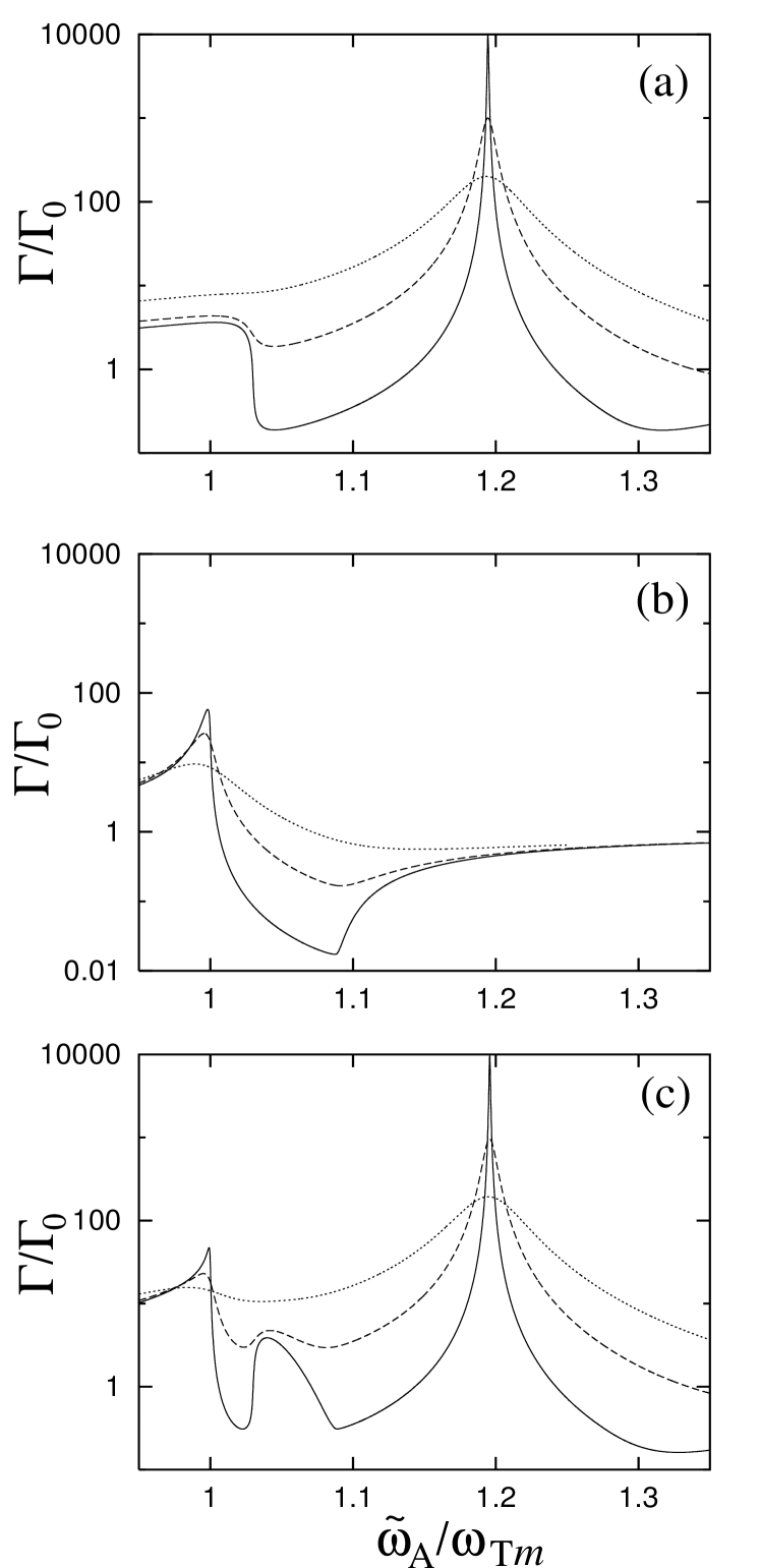
Figure 4: The decay rate $\Gamma$ as a function of the (shifted) atomic transition frequency $\tilde{\omega}_{\rm A}$ for an atom at the center of an empty sphere surrounded by single-resonance matter. (a) dielectric matter according to Eq. (10), (b) magnetic matter according to Eq. (11), and (c) magnetodielectric matter according to Eqs. (10) and (11). The diameter of the sphere is $2R$ $\!=$ $\!0.1\,\lambda_{{\rm T}m}$. The other parameters are the same as in Fig. 2.

Figure 5: The decay rate $\Gamma$ as a function of the (shifted) atomic transition frequency $\tilde{\omega}_{\rm A}$ for an atom at the center of an empty sphere surrounded by single-resonance matter. (a) dielectric matter according to Eq. (10), (b) magnetic matter according to Eq. (11), and (c) magnetodielectric matter according to Eqs. (10) and (11) [$\gamma_{e}/\omega_{{\rm T}m}$ $\!=$ $\gamma_{m}/\omega_{{\rm T}m}$ $\!=$ $\!0.001$, the other parameters are the same as in Fig. 2]. The values of the sphere diameter are $R$ $\!=$ $\!0.8\,\lambda_{{\rm T}m}$ (dotted lines), $0.4\,\lambda_{{\rm T}m}$ (dashed lines), and $0.1\,\lambda_{{\rm T}m}$ (solid lines).

In Fig. 4, a cavity is considered whose radius is much smaller than the transition wavelength ($2R/\lambda_{{\rm T}m}$ $\!=$ $\!0.1$). Comparing Fig. 4(a) with 4(b), we see that the frequency response of the decay rate in the dielectric band-gap zone is quite different from that in the magnetic band-gap zone. In the dielectric band-gap zone [Fig. 4(a)], a more or less abrupt decrease of $\Gamma$ below $\Gamma_{0}$ with increasing transition frequency is followed by an increase of $\Gamma$ to a maximum that can substantially exceed $\Gamma_{0}$. In the case of magnetic matter, [Fig. 4(b)], on the contrary, only a rather distorted band-gap zone is observed in which $\Gamma$ monotonously decreases below $\Gamma_{0}$. The maximum of enhancement of spontaneous decay in Fig. 4(a) is observed at the local-mode resonance associated with the small cavity, which may be regarded as being a defect of the otherwise homogeneous dielectric. This is obviously of the same nature as the donor and acceptor local modes discussed in Ref. Yablonovitch91 . In the regions where the dielectric and magnetic band-gap zones of the magnetodielectric in Fig. 4(c) do not overlap, the frequency response of the decay rate is dominated by the respective matter, i.e., the characteristic features are either dielectric or magnetic. The situation changes when the transition frequency is in the overlapping region, where LHM is realized. Since this region cannot longer be regarded as an effectively forbidden zone for propagating waves, the value of $\Gamma$ can become comparable with or even bigger than that of $\Gamma_{0}$. From Fig. 4(c) it is seen that entering the overlapping region from the magnetic side stops the decrease of $\Gamma$ on that side, thereby changing it to an increase. Similarly, the decrease of $\Gamma$ on the dielectric side stops and changes to an increase when the overlapping region is entered from the dielectric side.

Figure 5 illustrates the influence of the cavity radius on the decay rate for small cavities. Figure 5(a) reveals that when the value of $2R/\lambda_{{\rm T}m}$ changes from $2R/\lambda_{{\rm T}m}$ $\!=$ $\!0.1$ to $2R/\lambda_{{\rm T}m}$ $\!=$ $\!0.8$, then the maximum of the spontaneous decay rate associated with the local-mode resonance in dielectric matter shifts towards smaller transition frequencies, thereby being reduced. In the case of magnetic matter, increasing value of $2R/\lambda_{{\rm T}m}$ reduces the distortion of the band-gap zone, as is seen from Fig. 5(b). As expected, the frequency response of the decay rate shown in Fig. 5(c) for the case of magnetodielectric material including LHM combines, in a sense, the respective curves in Figs. 5(a) and 5(b).

V.2.3 Local-field corrections

For an atom in bulk material, the local field with which the atom really interacts can differ from the macroscopic field used in the derivation of the decay rate of the form given by Eq. (63). To include local-field corrections in the rate, one can use Eq. (69) and let the radius of the cavity tend to a value which is much smaller than the transition wavelength,

$$\frac{R\tilde{\omega}_{\rm A}}{c}=\frac{2\pi R}{\lambda_{\rm A}}\ll 1,$$ (70)

but still much larger than the distances between the medium constituents to ensure that the macroscopic theory applies. In this way we arrive at the real-cavity model frequently used in the literature Onsager36 ; Yablonovitch88 ; Glauber91 ; Scheel99 ; Tomas01 . The results shown in Fig. 4 may be regarded as being typical of the real-cavity model.

Expanding $\Gamma$ [Eq. (69)] in powers of $z$ $\!=$ $\!R\tilde{\omega}_{\rm A}/c$ we obtain

$$\frac{\Gamma}{\Gamma_{0}}={\rm Re}\,\biggl{[}\left(\frac{3\varepsilon}{1+2\varepsilon}\right)^{2}\mu n\biggr{]}+\frac{9{\rm Im}\,\varepsilon}{|1+2\varepsilon|^{2}}\left(\frac{c}{\tilde{\omega}_{\rm A}R}\right)^{3}$$ (71)

$$+\,{\textstyle\frac{9}{5}}\,{\rm Im}\left[\frac{\varepsilon(1+3\varepsilon+5\mu\varepsilon)}{(1+2\varepsilon)^{2}}\right]\left(\frac{c}{\tilde{\omega}_{\rm A}R}\right)+O(R),\qquad$$

which for nonmagnetic media reduces to results obtained earlier Scheel99 ; Tomas01 . Note that the actual value of $R$, which is undetermined within the real-cavity model, should be taken from the experiment. Equation (71) without the $O(R)$ term has to be employed with great care, because it fails when, for small absorption, the atomic transition frequency $\tilde{\omega}_{\rm A}$ becomes close to a medium resonance frequency such as $\omega_{{\rm T}e}$ or $\omega_{{\rm T}m}$, thus leading to a drastic increase of the first term in Eq. (71). The first three terms on the right-hand side in Eq. (71) reproduce the curves in Fig. 4 sufficiently well, except in the vicinities of $\omega_{{\rm T}e}$ and $\omega_{{\rm T}m}$. In particular, it can easily be checked that the position of the local-mode-assisted maximum of the decay rate in the dielectric band-gap zone is where $2\varepsilon(\tilde{\omega}_{\rm A})$ $\!\simeq$ $\!-1$.

For transition frequencies that are sufficiently far away from a medium resonance frequency and, in case of dielectric and magnetodielectric matter, the local-mode frequency, so that material absorption can be disregarded, the first term in Eq. (71) is the leading one, hence

$$\Gamma\simeq\left[\frac{3\varepsilon(\tilde{\omega}_{\rm A})}{1+2\varepsilon(\tilde{\omega}_{\rm A})}\right]^{2}{\rm Re}\,[\mu(\tilde{\omega}_{\rm A})n(\tilde{\omega}_{\rm A})]\Gamma_{0}.$$ (72)

In this case, the local-field correction simply results in multiplying the rate obtained for the case of nonabsorbing bulk material [Eq. (63)] by the factor $[3\varepsilon/(1$ $\!+$ $\!2\varepsilon)]^{2}$. Interestingly, this factor is exactly the same as that for dielectric material.

Inspection of the second and the third term in Eq. (71) shows that such a separation is no longer possible when material absorption must be taken into account. It should be pointed out that the second term proportional to $R^{-3}$ is purely dielectric, whereas the magnetization starts to come into play only via the third term proportional to $R^{-1}$. These two terms can be regarded as resulting from the near-field component and the induction-field component accompanying the decay of the excited atomic state. In particular for sufficiently small cavity size and strong (dielectric) absorption, the second term is the leading one, so that magnetodielectrics approximately give rise to the same decay rate as dielectrics:

$$\Gamma\simeq\frac{9{\rm Im}\,\varepsilon(\tilde{\omega}_{\rm A})}{|1+2\varepsilon(\tilde{\omega}_{\rm A})|^{2}}\left(\frac{c}{\tilde{\omega}_{\rm A}R}\right)^{3}\Gamma_{0}.$$ (73)

In this case, the decay may be regarded as being purely radiationless, with the energy being transferred from the excited atomic state to the surrounding medium mediated by the near field.

VI Summary and conclusions

It has been shown that the quantization scheme originally developed for the electromagnetic field in the presence of dielectric matter described in terms of a spatially varying, Kramers-Kronig-consistent permittivity Gruner95 ; Matloob95 ; Ho98 ; Tip97 ; Stefano00 ; Knoll01 can be extended to causal magnetodielectric matter, with special emphasis on the recently fabricated metamaterials, including LHMs that can exhibit a negative real part of the refractive index, thereby leading to a number of unusual properties. The quantization scheme is based on a source-quantity representation of the medium-assisted electromagnetic field in terms of the classical Green tensor and two independent infinite sets of appropriately chosen bosonic basis fields of the system that consists of the electromagnetic field and the medium, including a dissipative system. We have further shown that the minimal-coupling Hamiltonian governing the interaction of the medium-assisted electromagnetic field with additional charged particles can be obtained from the standard form, by expressing in it the potentials in terms of the bosonic basis fields. The theory can serve as basis for various studies, including generation and propagation of nonclassical radiation through magnetodielectric structures, Casimir forces between magnetodielectric bodies, or van-der-Waals force between atomic systems and magnetodielectric bodies.

As an example, we have applied the theory to the problem of the spontaneous decay of a two-level atom in the presence of arbitrarily configured, dispersing and absorbing media. In particular, we have shown that the theory naturally gives the decay rate and the frequency shift in terms of the classical Green tensor – formulas that are valid for any kind of geometry and material. To be more specific, we have studied the decay rate of an atom at the center of a cavity surrounded by a magnetodielectric, assuming a single-resonance permittivity and a single-resonance permeability of Drude-Lorentz type. LHM is realized for transition frequencies in the region where the dielectric and magnetic band-gap zones overlap, thereby the real parts of the permittivity and permeability becoming negative. When the transition frequency enter that region from the dielectric or magnetic side, then the typical band-gap properties such as enhancement of the spontaneous decay at the cavity resonances and inhibition between them gets lost and a decay rate comparable with that in free space can be observed. The calculations have been performed for both large and small cavities. In particular, if the diameter of the cavity becomes small compared to the transition wavelength of the atom, the system reduces to the real-cavity model for including local-field corrections in the decay rate of the atom in bulk material. We have discussed this case in detail both analytically and numerically and made contact with the results obtained from simple mode-decomposition arguments in case of positive permittivity and permeability.

For simplicity, all the calculations have been performed for isotropic magnetodielectric material, by assuming a scalar permittivity and a scalar permeability. The extension to anisotropic material is straightforward. It can be done in essentially the same way as for anisotropic dielectric material, by first transforming the permittivity and permeability tensors into their diagonal forms.

Appendix A Some properties of the Green tensor

Following Ref. Knoll01 , we regard the Green tensor as being the matrix elements in the position basis of a tensor-valued Green operator $\hat{\bm{G}}$ $\!=$ $\!\hat{\bm{G}}(\omega)$ in an abstract single-particle Hilbert space, $\bm{G}({\bf r},{\bf r}^{\prime},\omega)=$ $\langle{\bf r}|\hat{\bm{G}}|{\bf r}^{\prime}\rangle$, so that Eq. (23) can be regarded as the position-representation of the operator equation $\hat{\bm{H}}\hat{\bm{G}}=\hat{\bm{I}}$, where

$$\hat{\bm{H}}=-\hat{\bf p}\times\kappa(\hat{\bf r},\omega)\hat{\bf p}\times-\frac{\omega^{2}}{c^{2}}\varepsilon(\hat{{\bf r}},\omega)\hat{\bm{I}}.$$ (74)

Using the relations $\langle{\bf r}|\hat{\bf r}|{\bf r}^{\prime}\rangle$ $\!=$ $\!{\bf r}\delta({\bf r}-{\bf r}^{\prime})$, $\langle{\bf r}|\hat{\bf p}|{\bf r}^{\prime}\rangle$ $=$ $\!-i\bm{\nabla}\delta({\bf r}-{\bf r}^{\prime})$, and $\langle{\bf r}|\hat{\bm{I}}|{\bf r}^{\prime}\rangle$ $\!=$ $\!\bm{\delta}({\bf r}-{\bf r}^{\prime})$, we have

$$\bm{H}({\bf r},{\bf r}^{\prime},\omega)\equiv\langle{\bf r}|\hat{\bm{H}}|{\bf r}^{\prime}\rangle$$ (75)

$$=\bm{\nabla}\!\times\!\kappa({\bf r},\omega)\bm{\nabla}\times\delta({\bf r}\!-\!{\bf r}^{\prime})-\frac{\omega^{2}}{c^{2}}\,\varepsilon({\bf r},\omega)\bm{\delta}({\bf r}\!-\!{\bf r}^{\prime}),\qquad$$

which in Cartesian coordinates reads

$$H_{ij}({\bf r},{\bf r}^{\prime},\omega)=\biggl{\{}\partial^{r}_{j}\kappa({\bf r},\omega)\partial^{r}_{i}$$ (76)

$$-\left[\partial^{r}_{l}\kappa({\bf r},\omega)\partial^{r}_{l}+\frac{\omega^{2}}{c^{2}}\varepsilon({\bf r},\omega)\right]\delta_{ij}\biggr{\}}\delta({\bf r}-{\bf r}^{\prime}).\quad$$

Since $\hat{\bm{H}}$ is injective and thus an invertible one-to-one map between vector functions, we can write $\hat{\bm{G}}$ $\!=$ $\!\hat{\bm{H}}^{-1}$. Multiplying this equation by $\hat{\bm{H}}$ from the right, we have

$$\hat{\bm{G}}\hat{\bm{H}}=\hat{\bm{I}},$$ (77)

which in the position basis reads

$$\int{\rm d}^{3}{s}\,\langle{\bf r}|\hat{\bm{G}}|{\bf s}\rangle\langle{\bf s}|\hat{\bm{H}}|{\bf r^{\prime}}\rangle=\bm{\delta}({\bf r}-{\bf r}^{\prime}).$$ (78)

Recalling Eq. (76), we derive, on integrating by parts and taking into account that the Green tensor vanishes at infinity,

$$\int{\rm d}^{3}{s}\,G_{ik}({\bf r},{\bf s},\omega)H_{kj}({\bf s},{\bf r}^{\prime},\omega)$$ (79)

$$=\biggl{\{}\partial^{r^{\prime}}_{k}\kappa({\bf r}^{\prime},\omega)\partial^{r^{\prime}}_{j}-\left[\partial^{r^{\prime}}_{l}\kappa({\bf r}^{\prime},\omega)\partial^{r^{\prime}}_{l}+\frac{\omega^{2}}{c^{2}}\varepsilon({\bf r}^{\prime},\omega)\right]\delta_{kj}\bigg{\}}$$

$$\hskip 21.52771pt\times\,G_{ik}({\bf r},{\bf r}^{\prime},\omega)=\delta_{ij}({\bf r}-{\bf r}^{\prime}).$$

Interchanging the vector indices $i$ and $j$ and the spatial arguments ${\bf r}$ and ${\bf r}^{\prime}$, we obtain

$$\Big{\{}\partial^{r}_{k}\kappa({\bf r},\omega)\partial^{r}_{i}-\big{[}\partial^{r}_{l}\kappa({\bf r},\omega)\partial^{r}_{l}+\frac{\omega^{2}}{c^{2}}\varepsilon({\bf r},\omega)\big{]}\delta_{ki}\Big{\}}$$ (80)

$$\hskip 43.05542pt\times G_{jk}({\bf r}^{\prime},{\bf r},\omega)=\delta_{ij}({\bf r}-{\bf r}^{\prime}),$$

which, according to Eq. (23), is just the defining equation for $G_{kj}({\bf r},{\bf r}^{\prime},\omega)$. Thus, the reciprocity relation (24) is proved valid.

To prove the integral relation (III), we introduce operators $\hat{\bm{O}}^{\ddagger}$ by $\bigl{(}\hat{O}^{\ddagger}\bigr{)}_{ij}$ $=\bigl{(}\hat{O}_{ji}\bigr{)}^{\dagger}$ $=\hat{O}^{\dagger}_{ji}$. From Eq. (77) it then follows that

$$\hat{\bm{H}}^{\ddagger}\hat{\bm{G}}^{\ddagger}=\hat{\bm{I}}.$$ (81)

Multiplying Eq. (77) from the right by $\hat{\bm{G}}^{\ddagger}$ and Eq. (81) from the left by $\hat{\bm{G}}$ and subtracting the resulting equations from each other, we obtain

$$\hat{\bm{G}}\bigl{(}\hat{\bm{H}}-\hat{\bm{H}}^{\ddagger}\bigr{)}\hat{\bm{G}}^{\ddagger}=\hat{\bm{G}}^{\ddagger}-\hat{\bm{G}},$$ (82)

which in the position basis reads

$$\begin{split}\int&\!{\rm d}^{3}s\!\int\!{\rm d}^{3}s^{\prime}\,G_{im}({\bf r},{\bf s},\omega)[H_{mn}({\bf s},{\bf s}^{\prime},\omega)\\[2.15277pt] &-H^{\ast}_{nm}({\bf s}^{\prime},{\bf s},\omega)]G^{\ast}_{nj}({\bf s}^{\prime},{\bf r}^{\prime},\omega)=-2i{\rm Im}G_{ij}({\bf r},{\bf r}^{\prime},\omega).\end{split}$$ (83)

Note that $\langle{\bf r}|\hat{H}_{mn}^{\ddagger}|{\bf r}^{\prime}\rangle$ $\!=$ $\!H_{nm}^{\ast}({\bf r}^{\prime},{\bf r},\omega)$ and $\langle{\bf r}|\hat{G}_{ij}^{\ddagger}|{\bf r}^{\prime}\rangle$ $\!=$ $\!G_{ji}^{\ast}({\bf r}^{\prime},{\bf r},\omega)$. Inserting Eq. (76) into Eq. (83), after some manipulation we derive

$$\int{\rm d}^{3}s\,\Bigl{\{}{\rm Im}\,\kappa\,({\bf s},\omega)\partial^{s}_{n}G_{im}({\bf r},{\bf s},\omega)$$ (84)

$$\times\,[\partial^{s}_{m}G^{\ast}_{nj}({\bf s},{\bf r}^{\prime},\omega)-\partial^{s}_{n}G^{\ast}_{mj}({\bf s},{\bf r}^{\prime},\omega)]$$

$$\hskip 8.61108pt+\,\frac{\omega^{2}}{c^{2}}\,{\rm Im}\,\varepsilon({\bf s},\omega)G_{im}({\bf r},{\bf s},\omega)G^{\ast}_{mj}({\bf s},{\bf r}^{\prime},\omega)\Bigr{\}}\quad$$

$$\hskip 17.22217pt={\rm Im}G_{ij}({\bf r},{\bf r}^{\prime},\omega),$$

which is just Eq. (III) in Cartesian coordinates.

To examine the asymptotic behaviour of the Green tensor in the upper half of the complex $\omega$-plane as $|\omega|\to\infty$ and $|\omega|\to 0$, we introduce the tensor-valued projectors

$$\hat{\bm{I}}^{\perp}=\hat{\bm{I}}-\hat{\bm{I}}^{\parallel},\quad\hat{\bm{I}}^{\parallel}=\frac{\hat{\bf p}\otimes\hat{\bf p}}{\hat{\bf p}^{2}}$$ (85)

[note that $\langle{\bf r}|\hat{\bm{I}}^{\perp(\parallel)}|{\bf r}^{\prime}\rangle$ $\!=$ $\!\bm{\delta}^{\perp(\parallel)}({\bf r}-{\bf r}^{\prime})$], and decompose $\hat{\bm{G}}$ as Knoll01 ,

$$\hat{\bm{G}}=\hat{\bm{H}}^{-1}=\hat{\bm{I}}^{\parallel}(\hat{\bm{I}}^{\parallel}\hat{\bm{H}}\hat{\bm{I}}^{\parallel})^{-1}\hat{\bm{I}}^{\parallel}$$ (86)

$$\hskip 8.61108pt+\,\bigl{[}\hat{\bm{I}}^{\perp}-\hat{\bm{I}}^{\parallel}(\hat{\bm{I}}^{\parallel}\hat{\bm{H}}\hat{\bm{I}}^{\parallel})^{-1}\hat{\bm{I}}^{\parallel}\hat{\bm{H}}\hat{\bm{I}}^{\perp}\bigr{]}\hat{\bm{K}}$$

$$\hskip 21.52771pt\times\,\bigl{[}\hat{\bm{I}}^{\perp}-\hat{\bm{I}}^{\perp}\hat{\bm{H}}\hat{\bm{I}}^{\parallel}(\hat{\bm{I}}^{\parallel}\hat{\bm{H}}\hat{\bm{I}}^{\parallel})^{-1}\hat{\bm{I}}^{\parallel}\bigr{]},$$

where

$$\hat{\bm{K}}=\bigl{[}\hat{\bm{I}}^{\perp}\hat{\bm{H}}\hat{\bm{I}}^{\perp}-\hat{\bm{I}}^{\perp}\hat{\bm{H}}\hat{\bm{I}}^{\parallel}(\hat{\bm{I}}^{\parallel}\hat{\bm{H}}\hat{\bm{I}}^{\parallel})^{-1}\hat{\bm{I}}^{\parallel}\hat{\bm{H}}\hat{\bm{I}}^{\perp}\bigr{]}^{-1}.\quad$$ (87)

Recalling that $\varepsilon({\bf r},\omega),\,\mu({\bf r},\omega)$ $\!\to$ $\!1$ as $|\omega|$ $\!\to$ $\!\infty$, we easily see that the high-frequency limits of $\hat{\bm{H}}$ and $\hat{\bm{G}}$ are the same as for dielectric material, thus Knoll01

$$\lim_{|\omega|\to\infty}\frac{\omega^{2}}{c^{2}}\,{\bm{G}}({\bf r},{\bf r}^{\prime},\omega)=-{\bm{\delta}}({\bf r}-{\bf r}^{\prime}).$$ (88)

To find the low-frequency limit of $\hat{\bm{G}}$, we note that the second term in Eq. (86) is regular. To study the first term, we distinguish between two cases.
(i) The first term of $\hat{\bm{H}}$ in Eq. (74) is transverse,

$$-\hat{\bm{I}}^{\parallel}\hat{\bf p}\times\kappa(\hat{\bf r},\omega)\hat{\bf p}\times=-\hat{\bf p}\times\kappa(\hat{\bf r},\omega)\hat{\bf p}\times\hat{\bm{I}}^{\parallel}=0,$$ (89)

and therefore does not contribute to $\hat{\bm{I}}^{\parallel}\hat{\bm{H}}\hat{\bm{I}}^{\parallel}$. It then follows that the same low-frequency behaviour as in the case of dielectric matter is observed, thus Knoll01

$$\lim_{|\omega|\to 0}\frac{\omega^{2}}{c^{2}}\,\hat{\bm{G}}=-\hat{\bm{I}}^{\parallel}[\hat{\bm{I}}^{\parallel}\varepsilon(\hat{\bf r},\omega=0)\hat{\bm{I}}^{\parallel}]^{-1}\hat{\bm{I}}^{\parallel},$$ (90)

i.e., because $\varepsilon({\bf r},\omega=0)$ $\!\neq$ $\!0$,

$$\lim_{|\omega|\to 0}\frac{\omega^{2}}{c^{2}}\,\bm{G}({\bf r},{\bf r}^{\prime},\omega)=\bm{M},\qquad M_{ij}<\infty.$$ (91)

(ii) Equation (89) is not valid, so that the first term of $\hat{\bm{H}}$ in Eq. (74) contributes to $\hat{\bm{I}}^{\parallel}\hat{\bm{H}}\hat{\bm{I}}^{\parallel}$. Since $\mu({\bf r},\omega=0)$ $\!\neq$ $\!0$ [thus $\kappa({\bf r},\omega$ $\!=$ $\!0)$ being finite], we find that

$$\lim_{|\omega|\to 0}\bm{G}({\bf r},{\bf r}^{\prime},\omega)=\bm{N},\qquad N_{ij}<\infty.$$ (92)

Appendix B Commutation relations

By using Eqs. (22), (32), the commutation relations (31) and (31), and the integral relation (III), we derive

$$\bigl{[}\underline{\hat{E}}_{i}({\bf r},\omega),\underline{\hat{E}}^{\dagger}_{j}({\bf r}^{\prime},\omega^{\prime})\bigr{]}$$ (93)

$$\hskip 8.61108pt=\frac{\hbar\omega^{2}}{\pi\varepsilon_{0}c^{2}}\,{\rm Im}\,G_{ij}({\bf r},{\bf r}^{\prime},\omega)\,\delta(\omega-\omega^{\prime}),$$

$$\bigl{[}\underline{\hat{E}}_{i}({\bf r},\omega),\underline{\hat{E}}_{j}({\bf r}^{\prime},\omega^{\prime})\bigr{]}=\bigl{[}\underline{\hat{E}}_{i}^{\dagger}({\bf r},\omega),\underline{\hat{E}}^{\dagger}_{j}({\bf r}^{\prime},\omega^{\prime})\bigr{]}=0.$$ (94)

From Eqs. (34), (93), and (94) it is easily seen that the commutation relations (35) are valid. Moreover, we find that, on recalling that $\bm{G}^{\ast}({\bf r},{\bf r}^{\prime},\omega)$ $=\bm{G}({\bf r},{\bf r}^{\prime},-\omega^{\ast})$,

$$\bigl{[}\varepsilon_{0} \hat{E}_{i}({\bf r}),\hat{A}_{j}({\bf r}^{\prime})\bigr{]}$$

$$=\int{\rm d}^{3}s\biggl{[}\frac{2i\hbar}{\pi}\int_{0}^{\infty}{\rm d}\omega\,\frac{\omega}{c^{2}}\,{\rm Im}\,G_{ik}({\bf r},{\bf s},\omega)\biggr{]}\delta_{kj}^{\perp}({\bf s}-{\bf r}^{\prime})$$

$$=\int{\rm d}^{3}s\biggl{[}\frac{\hbar}{\pi}\,{\cal P}\int_{-\infty}^{\infty}{\rm d}\omega\,\frac{\omega}{c^{2}}\,G_{ik}({\bf r},{\bf s},\omega)\biggr{]}\delta_{kj}^{\perp}({\bf s}-{\bf r}^{\prime})$$

$$=\frac{\hbar}{\pi}\,{\cal P}\int_{-\infty}^{\infty}\frac{{\rm d}\omega}{\omega}\,\frac{\omega^{2}}{c^{2}}\,\langle{\bf r}|\hat{\bm{G}}\hat{\bm{I}}^{\perp}|{\bf r}^{\prime}\rangle_{ij}$$ (95)

(${\cal P}$, principal part). Since the Green tensor is analytic in the upper half of the complex $\omega$-plane with the asymptotic behaviour according to Eq. (88), the frequency integral in Eq. (B) can be evaluated by contour integration along an infinitely small half-circle around $\omega$ $\!=$ $\!0$, and along an infinitely large half-circle $|\omega|$ $\!\to$ $\!\infty$. Taking into account that the Green tensor either has only longitudinal components in the limit $|\omega|$ $\!\to$ $\!0$, cf. Eq. (90), and hence $\omega/c\hat{\bm{G}}\hat{\bm{I}}^{\perp}$ $\!\to$ $\!0$, or is well-behaved, cf. Eq. (92), we see that the integral along the infinitely small half-circle vanishes. Recalling Eq. (88), we then readily find

$$\bigl{[}\varepsilon_{0}\hat{E}_{i}({\bf r}),\hat{A}_{j}({\bf r}^{\prime})\bigr{]}=i\hbar\delta_{ij}^{\perp}({\bf r}-{\bf r}^{\prime}).$$ (96)

Since $\hat{\bf B}({\bf r})$ $\!=$ $\!{\bm{\nabla}}\times\hat{\bf A}({\bf r})$, from Eq. (96) it follows that

$$\bigl{[}\varepsilon_{0}\hat{E}_{i}({\bf r}),\hat{B}_{j}({\bf r}^{\prime})\bigr{]} = -i\hbar\epsilon_{ijk}\partial^{r}_{k}\delta({\bf r}-{\bf r}^{\prime}),$$ (97)

i.e., Eq. (36). It is then not difficult to see that the commutation relation (96) implies

$$\bigl{[}\hat{\varphi}({\bf r}),\hat{A}_{i}({\bf r}^{\prime})\bigr{]}=\bigl{[}\hat{\varphi}({\bf r}),\hat{B}_{i}({\bf r}^{\prime})\bigr{]}=0.$$ (98)

To evaluate commutators involving the displacement field and the magnetic field, recall Eqs. (16) – (19). Using the relations presented above, we derive

$$\bigl{[}\hat{D}_{i}({\bf r}),\hat{D}_{j}({\bf r}^{\prime})\bigr{]}=0,$$ (99)

$$\bigl{[}\hat{H}_{i}({\bf r}),\hat{H}_{j}({\bf r}^{\prime})\bigr{]}=0,$$ (100)

and

$$\bigl{[}\hat{D}_{i}({\bf r}),\mu_{0}\hat{H}_{j}({\bf r}^{\prime})\bigr{]}=-i\hbar\epsilon_{ijk}\partial^{r}_{k}\delta({\bf r}-{\bf r}^{\prime}).$$ (101)

Note that Eq. (101) follows by using similar arguments as in the derivation of Eq. (96) from Eq. (B). A similar calculation leads to

$$\displaystyle\bigl{[}\hat{D}_{i}({\bf r}),\hat{A}_{j}({\bf r}^{\prime})\bigr{]}=i\hbar\delta_{ij}^{\perp}({\bf r}-{\bf r}^{\prime}),$$ (102)

$$\displaystyle\bigl{[}\hat{H}_{i}({\bf r}),\hat{A}_{j}({\bf r}^{\prime})\bigr{]}=\bigl{[}\hat{D}_{i}({\bf r}),\hat{\varphi}({\bf r}^{\prime})\bigr{]}=\bigl{[}\hat{H}_{i}({\bf r}),\hat{\varphi}({\bf r}^{\prime})\bigr{]}=0.$$

By combining Eqs. (102) – (B) with Eqs. (96) and (98), it is not difficult to verify that polarization and magnetization commute with the introduced potentials as well as among themselves.

Appendix C Heisenberg equations of motion

By using the Hamiltonian (41) and recalling the definitions of the medium-assisted field quantities in terms of the basic fields $\hat{f}_{\lambda i}({\bf r},\omega)$ the basic-field commutation relations (31) and (31), the commutation relations that have been derived from them, and the standard commutation relations for the particle coordinates and canonical momenta, it is straightforward to prove that the theory yields both the correct Maxwell equations (47) and (48) and the correct Newtonian equation of motion (51).

Let us begin with the Maxwell equations. We derive on recalling Eqs. (40) and (34) together with Eqs. (22) and (32) and the commutation relations (31) and (31),

$$\dot{\hat{\vec{B}}}({\bf r},t) = \frac{1}{i\hbar}\,\bigl{[}\hat{\vec{B}}({\bf r},t),\hat{H}\bigr{]}$$ (104)

$$= \bm{\nabla}\!\times\!\int_{0}^{\infty}\!\!{\rm d}\omega\,\frac{1}{i\hbar}\bigl{[}\underline{\hat{\bf A}}({\bf r},\omega),\hat{H}\bigr{]}+{\rm H.c.}$$

$$= -\bm{\nabla}\times\hat{\bf E}({\bf r})=-\bm{\nabla}\times\hat{\vec{E}}({\bf r}),$$

which is Eq. (47). To derive the equation of motion for the displacement field, we have to consider several commutators according to

$$\dot{\hat{\vec{D}}}({\bf r})=\frac{1}{i\hbar}\,\bigl{[}\hat{\vec{D}}({\bf r},t),\hat{H}\bigr{]}$$ (105)

$$=\frac{1}{i\hbar}\int\!{\rm d}^{3}r^{\prime}\!\int_{0}^{\infty}\!\!{\rm d}\omega\,\hbar\omega\!\sum_{\lambda=e,m}\bigl{[}\hat{\bf D}({\bf r}),\hat{\bf f}_{\lambda}^{\dagger}({\bf r}^{\prime},\omega)\hat{\bf f}_{\lambda}({\bf r}^{\prime},\omega)\bigr{]}$$

$$\hskip 8.61108pt+\,\frac{1}{i\hbar}\sum_{\alpha}\frac{1}{2m_{\alpha}}\left[\hat{\bf D}({\bf r}),\bigl{[}\hat{\bf p}_{\alpha}-q_{\alpha}\hat{\bf A}(\hat{\bf r}_{\alpha})\bigr{]}^{2}\right]$$

$$\hskip 8.61108pt-\,\frac{\varepsilon_{0}}{i\hbar}\sum_{\alpha}\frac{1}{2m_{\alpha}}\left[\bm{\nabla}\hat{\varphi}_{\rm A}({\bf r}),\bigl{[}\hat{\bf p}_{\alpha}-q_{\alpha}\hat{\bf A}(\hat{\bf r}_{\alpha})\bigr{]}^{2}\right].\qquad$$

The first commutator in Eq. (105) can easily be found by recalling the definitions of displacement and magnetic fields as

$$\frac{1}{i\hbar}\int\!{\rm d}^{3}r^{\prime}\!\int_{0}^{\infty}\!\!{\rm d}\omega\,\hbar\omega\!\sum_{\lambda=e,m}\bigl{[}\hat{\bf D}({\bf r}),\hat{\bf f}_{\lambda}^{\dagger}({\bf r}^{\prime},\omega)\hat{\bf f}_{\lambda}({\bf r}^{\prime},\omega)\bigr{]}$$ (106)

$$=-\int_{0}^{\infty}{\rm d}\omega\,i\omega\hat{\underline{\bf D}}({\bf r},\omega)+{\rm H.c.}=\bm{\nabla}\times\hat{\vec{H}}({\bf r}).\qquad$$

Applying the commutation relation (102), and recalling the definition of the current density, we find that the second term on the right-hand side of Eq. (105) can be written as

$$\frac{1}{i\hbar}\sum_{\alpha}\frac{1}{2m_{\alpha}}\left[\hat{\bf D}({\bf r}),\bigl{[}\hat{\bf p}_{\alpha}-q_{\alpha}\hat{\bf A}(\hat{\bf r}_{\alpha})\bigr{]}^{2}\right]=-\hat{\bf j}^{\perp}_{\rm A}({\bf r}),$$ (107)

where the Newtonian equation of motion (50) has been used which follows directly from the Hamiltonian (41). Finally, standard commutation relations together with the definitions of the scalar potential, Eqs. (42) and (43), and the current density, Eq. (49) together with Eq. (50), lead to

$$-\frac{\varepsilon_{0}}{i\hbar}\sum_{\alpha}\frac{1}{2m_{\alpha}}[\bm{\nabla}\hat{\varphi}_{\rm A}({\bf r}),[\hat{\bf p}_{\alpha}-q_{\alpha}\hat{\bf A}(\hat{\bf r}_{\alpha})]^{2}]=-\hat{\bf j}^{\parallel}_{\rm A}({\bf r}).$$ (108)

Inserting Eqs. (106) – (108) into Eq. (105), we arrive at Eq. (48).

In order to prove Eq. (51), we consider the equation

$$m_{\alpha}\ddot{\hat{{\bf r}}}_{\alpha}=\frac{1}{i\hbar}\bigl{[}\hat{\bf p}_{\alpha}-q_{\alpha}\hat{\bf A}(\hat{\bf r}_{\alpha}),\hat{H}\bigr{]}$$ (109)

$$=-\frac{q_{\alpha}}{i\hbar}\!\int\!{\rm d}^{3}r\!\int_{0}^{\infty}\!\!{\rm d}\omega\,\hbar\omega\!\sum_{\lambda=e,m}\bigl{[}\hat{\bf A}(\hat{\bf r}_{\alpha}),\hat{\bf f}_{\lambda}^{\dagger}({\bf r},\omega)\hat{\bf f}_{\lambda}({\bf r},\omega)\bigr{]}$$

$$\hskip 8.61108pt+\,\frac{1}{i\hbar}\sum_{\beta}\frac{1}{2m_{\beta}}\left[\hat{\bf p}_{\alpha}-q_{\alpha}\hat{\bf A}(\hat{\bf r}_{\alpha}),\bigl{[}\hat{\bf p}_{\beta}-q_{\beta}\hat{\bf A}(\hat{\bf r}_{\beta})\bigr{]}^{2}\right]$$

$$\hskip 8.61108pt+\,\frac{1}{2i\hbar}\int{\rm d}^{3}r\,\bigl{[}\hat{\bf p}_{\alpha},\hat{\rho}_{\rm A}({\bf r})\hat{\varphi}_{\rm A}({\bf r})\bigr{]}$$

$$\hskip 8.61108pt+\,\frac{1}{i\hbar}\int{\rm d}^{3}r\,\bigl{[}\hat{\bf p}_{\alpha},\hat{\rho}_{\rm A}({\bf r})\hat{\varphi}({\bf r})\bigr{]}.$$

The first term on the right-hand side of Eq. (109) is again

$$-\frac{q_{\alpha}}{i\hbar}\!\int\!{\rm d}^{3}r\!\int_{0}^{\infty}\!\!{\rm d}\omega\,\hbar\omega\!\sum_{\lambda=e,m}\bigl{[}\hat{\bf A}(\hat{\bf r}_{\alpha}),\hat{\bf f}_{\lambda}^{\dagger}({\bf r},\omega)\hat{\bf f}_{\lambda}({\bf r},\omega)\bigr{]}$$ (110)

$$\hskip 43.05542pt=i\omega q_{\alpha}\hat{\bf A}(\hat{\bf r}_{\alpha})=q_{\alpha}\hat{\bf E}^{\perp}(\hat{\bf r}_{\alpha}).\qquad$$

The second term gives rise to two terms,

$$\frac{1}{i\hbar}\sum_{\beta}\frac{1}{2m_{\beta}}\left[\hat{\bf p}_{\alpha},\bigl{[}\hat{\bf p}_{\beta}-q_{\beta}\hat{\bf A}(\hat{\bf r}_{\beta})\bigr{]}^{2}\right]$$ (111)

$$={\textstyle\frac{1}{2}}q_{\alpha}\left\{\dot{\hat{\bf r}}_{\alpha}\hat{\bf A}(\hat{\bf r}_{\alpha})\otimes\overleftarrow{\bm{\nabla}}+\bm{\nabla}\otimes\hat{\bf A}(\hat{\bf r}_{\alpha})\dot{\hat{\bf r}}_{\alpha}\right\}\qquad$$

and

$$-\frac{q_{\alpha}}{i\hbar}\sum_{\beta}\frac{1}{2m_{\beta}}\left[\hat{\bf A}(\hat{\bf r}_{\alpha}),\bigl{[}\hat{\bf p}_{\beta}-q_{\beta}\hat{\bf A}(\hat{\bf r}_{\beta})\bigr{]}^{2}\right]$$ (112)

$$=-{\textstyle\frac{1}{2}}q_{\alpha}\left\{\dot{\hat{\bf r}}_{\alpha}\bm{\nabla}\otimes\hat{\bf A}(\hat{\bf r}_{\alpha})+\hat{\bf A}(\hat{\bf r}_{\alpha})\otimes\dot{\hat{\bf r}}_{\alpha}\overleftarrow{\bm{\nabla}}\right\},\qquad$$

and thus

$$\frac{1}{i\hbar}\sum_{\beta}\frac{1}{2m_{\beta}}\left[\hat{\bf p}_{\alpha}-q_{\alpha}\hat{\bf A}(\hat{\bf r}_{\alpha}),\bigl{[}\hat{\bf p}_{\beta}-q_{\beta}\hat{\bf A}(\hat{\bf r}_{\beta})\bigr{]}^{2}\right]$$ (113)

$$={\textstyle\frac{1}{2}}q_{\alpha}\left[\dot{\hat{{\bf r}}}_{\alpha}\times\hat{\vec{B}}({\bf r}_{\alpha})-\hat{\vec{B}}({\bf r}_{\alpha})\times\dot{\hat{{\bf r}}}_{\alpha}\right].\qquad$$

By means of Eqs. (39) and (42) one can see that the last two terms in Eq. (109) can be rewritten as

$$\displaystyle\frac{1}{2i\hbar}\int{\rm d}^{3}r\,\bigl{[}\hat{\bf p}_{\alpha},\hat{\rho}_{\rm A}({\bf r})\hat{\varphi}_{\rm A}({\bf r})\bigr{]}=-q_{\alpha}\bm{\nabla}\hat{\varphi}_{\rm A}({\bf r}_{\alpha}),$$ (114)

$$\displaystyle\frac{1}{i\hbar}\int{\rm d}^{3}r\,\bigl{[}\hat{\bf p}_{\alpha},\hat{\rho}_{\rm A}({\bf r})\hat{\varphi}({\bf r})\bigr{]}=q_{\alpha}\hat{\bf E}^{\parallel}(\hat{\bf r}_{\alpha}).$$ (115)

Inserting Eqs. (110), (113) – (115) into Eq. (109) and making use of Eq. (44), we just arrive at Eq. (51).

References

• (1) V. G. Veselago, Sov. Phys. Usp. 10, 509 (1968).
• (2) D. R. Smith, W. J. Padilla, D. C. Vier, S. C. Nemat-Nasser, S. Shultz, Phys. Rev. Lett. 84, 4184 (2000); R. A. Shelby, D. R. Smith, S. C. Nemat-Nasser, S. Shultz, Appl. Phys. Lett. 78, 489 (2001).
• (3) R. A. Shelby, D. R. Smith, and S. Shultz, Science 292, 77 (2001).
• (4) R. Marqués, J. Martel, F. Mesa, and F. Medina, Phys. Rev. Lett. 89, 183901 (2002)
• (5) A. Grbic and G. V. Eleftheriades, J. Appl. Phys. 92, 5930 (2002).
• (6) C. G. Parazzoli, R. B. Greegor, K. Li, B. E. C. Koltenbah, and M. Tanielian, Phys. Rev. Lett. 90, 107401 (2003); K. Li, S. J. McLean, R. B. Greegor, C. G. Parazzoli, and M. H. Tanielian, App. Phys. Lett. 82, 2535 (2003); A. A. Houck, J. B. Brock, and I. L. Chuang, Phys. Rev. Lett. 90, 137401 (2003).
• (7) L. V. Panina, A. N. Grigorenko, and D. P. Makhnovskiy, Phys. Rev. B 66, 155411 (2002).
• (8) M. L. Povinelli, S. G. Johnson, J. D. Joannopoulos, and J. B. Pendry, Appl. Phys. Lett. 82, 1069 (2003).
• (9) D. R. Smith and N. Kroll, Phys. Rev. Lett. 85, 2933 (2000).
• (10) J. B. Pendry, Phys. Rev. Lett. 85, 3966 (2000).
• (11) G. W. ’t Hooft, Phys. Rev. Lett. 87, 249701 (2001); J. B. Pendry, ibid., 249702 (2001); J. M. Williams, ibid., 249703 (2001); J. B. Pendry, ibid., 249704 (2001); P. Markoš and C. M. Soukoulis, Phys. Rev. B 65, 033401 (2001); P. Markoš, I. Rousochatzakis, and C. M. Soukoulis, Phys. Rev. E 66, 045601(R) (2002); P. M. Valanju, R. M. Walser, and A. P. Valanju, Phys. Rev. Lett. 88, 187401 (2002); A. L. Pokrovsky and A. L. Efros, ibid. 89, 093901 (2002); J. Pacheco, Jr., T. M. Grzegorczyk, B.-I. Wu, Y. Zhang, and J. A. Kong, ibid., 257401 (2002); N. Fang and X. Zhang, Appl. Phys. Lett. 82, 161 (2003); G. Gómez-Santos, Phys. Rev. Lett. 90, 077401 (2003); D. R. Smith and D. Schurig, ibid., 077405 (2003); J. Li, L. Zhou, C. T. Chan, and P. Sheng, ibid., 083901 (2003); S. Foteinopoulou, E. N. Economou, and C. M. Soukoulis, ibid., 107402 (2003); S. A. Cummer, Appl. Phys. Lett. 82, 1503 (2003); ibid., 2008 (2003); D. R. Smith, D. Schurig, M. Rosenbluth, and S. Schultz, ibid., 1506 (2003); P. F. Loschialpo, D. L. Smith, D. W. Forester, F. J. Rachford, and J. Schelleng, Phys. Rev. E 67, 025602 (2003).
• (12) R. W. Ziolkowski and E. Heyman, Phys. Rev. E 64, 056625 (2001).
• (13) N. Garcia and M. Nieto-Vesperinas, Phys. Rev. Lett. 88, 207403 (2002); Opt. Lett. 27, 885 (2002).
• (14) T. Gruner and D.-G. Welsch, Third Workshop on Quantum Field Theory under the Influence of External Conditions (Leipzig, 1995) [B.G. Teubner Verlagsgesellschaft, Stuttgart$\cdot$Leipzig, 1996]; Phys. Rev. A 53, 1818 (1996).
• (15) R. Matloob, R. Loudon, S.M. Barnett, and J. Jeffers, Phys. Rev. A 52, 4823 (1995); R. Matloob and R. Loudon, ibid. 53, 4567 (1996).
• (16) Ho Trung Dung, L. Knöll, and D.-G. Welsch, Phys. Rev. A 57, 3931 (1998); S. Scheel, L. Knöll, and D.-G. Welsch, ibid. 58, 700 (1998).
• (17) A. Tip, Phys. Rev. A 56, 5022 (1997); ibid. 57, 4818 (1998); A. Tip, L. Knöll, S. Scheel, and D.-G. Welsch, ibid. 63, 043806 (2001).
• (18) O. D. Stefano, S. Savasta, and R. Girlanda, Phys. Rev. A 61, 023803 (2000).
• (19) L. Knöll, S. Scheel, and D.-G. Welsch, in Coherence and Statistics of Photons and Atoms, edited by J. Peřina (John Wiley & Son, New York, 2001) p. 1; e-print quant-ph/0006121.
• (20) E. Yablonovitch, T. J. Gmitter, and R. Blatt, Phys. Rev. Lett. 61, 2546 (1988).
• (21) S. M. Barnett, B. Huttner, R. Loudon, and R. Matloob, J. Phys. A 29, 3763 (1996).
• (22) L. D. Landau and E. M. Lifshitz, Electrodynamics of Continuous Media (Pergamon Press, 1960).
• (23) R. Ruppin, Phys. Lett. A 299, 309 (2002).
• (24) J. B. Pendry, A. J. Holden, D. J. Robbins, and W. J. Stewart, IEEE Trans. Microwave Theory Tech. 47, 2075 (1999).
• (25) A.A. Abrikosov, L.P. Gorkov, and I.E. Dzyaloshinski Methods of Quantum Field Theory in Statistical Physics (Dover, New York, 1963).
• (26) Ho Trung Dung, L. Knöll, and D.-G. Welsch, Phys. Rev. A 62, 053804 (2000); in Recent Research Developments in Optics, Vol. 1 (Research Signpost, Trivandrum, India, 2001) p. 225.
• (27) Ho Trung Dung, L. Knöll, and D.-G. Welsch, Phys. Rev. A 66, 063810 (2002).
• (28) R.R. Chance, A.Prock, and R. Sylbey, Adv. Chem. Phys. 37, 1 (1978).
• (29) V. V. Klimov, Opt. Commun. 211, 183 (2002).
• (30) L. W. Li, P. S. Kooi, M. S. Leong, and T. S. Yeo, IEEE Trans. Microwave Theory Tech. 42, 2302 (1994); C.-T. Tai, Dyadic Green Functions in Electromagnetic Theory (IEEE Press, New York, 1994).
• (31) S. Scheel, L. Knöll, and D.-G. Welsch, Phys. Rev. A 60, 4094 (1999).
• (32) E. Yablonovitch, T. J. Gmitter, R. D. Meade, A. M. Rappe, K. D. Brommer, and J. D. Joannopoulos, Phys. Rev. Lett. 67, 3380 (1991).
• (33) L. Onsager, J. Am. Chem. Soc. 58, 1486 (1936).
• (34) R.J. Glauber and M. Lewenstein, Phys. Rev. A 43, 467 (1991).
• (35) M. S. Tomaš, Phys. Rev. A 63, 053811 (2001).