Photon Added Detection

Abstract

The production of conditional quantum states and quantum operations based on the result of measurement is now seen as a key tool in quantum information and metrology. We propose a new type of photon number detector. It functions non-deterministically, but when successful, it has high fidelity. The detector, which makes use of an $n$-photon auxiliary Fock state and high efficiency Homodyne detection, allows a tunable tradeoff between fidelity and probability. By sacrificing probability of operation, an excellent approximation to a photon number detector is achieved.

I Introduction

In quantum theory, measurements encapsulate our observation of nature. They are the link between the abstract machinery of the theory and its observational consequences. Because of this, it is not surprising that often new measurement techniques and strategies can drive new applications. Moreover, the production of conditional quantum states and quantum operations based on the results of measurement is now seen as a key tool in realizing quantum information processing goals klm ; 99gottesman390 . In optical schemes, conditional measurements provide an effective nonlinearity that allows optical quantum gates to be fashioned klm ; 01pittman062311 ; 02ralph012314 ; 0110144 ; 0110115 , and the creation of highly entangled states suitable for quantum metrology 01lee030101 ; 02kok052104 ; 02fiurasek053818 ; 02zou014102 .

Often, however, the ideal measurements envisioned in theoretical proposals are not so easily realized experimentally. Linear optics quantum computation schemes such as in klm , require high efficiency selective detectors (detectors able to distinguish between zero, one and several photons). The most promising detector candidate in this regard is the visible-light photon counter (VLPC) 99kim902 ; 99takeuchi1063 which has achieved efficiencies of the order of 88%. Unfortunately these detectors require extreme operating conditions and suffer from high dark-count rates.

In this manuscript we introduce the idea of a non-deterministic detector based on photon added detection (PAD), where we make use of high efficiency homodyne detection and mix the input state with an $|n\rangle$ Fock state prior to detection. This detector works non-deterministically, and there is an essential trade-off between the probability that the detector works and the degree to which the detector functions as an $n$-Fock state projector. When the detector fails, this is clearly signalled in the output. The essence of the detecting scheme is based on the observation that if we use homodyne detection and post-select within a narrow band of $2\Delta$ around $x=0$ then the detection will only be sensitive to even photon numbers, see figure 1. By careful use of quantum interference, we can make the detector act like a projector onto a particular photon number.

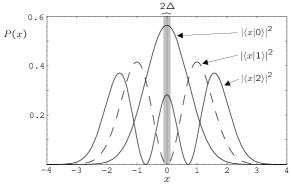
Figure 1: The probability density of getting a particular $x$ value if we measure the $X$ quadrature using homodyne detection. Results shown for various initial Fock states.

The structure of the paper is as follows. First we will introduce the scheme in general, then focus on the limiting case where $\Delta=0$ to motivate its function. We then consider the effect of a finite $\Delta$ and discuss the trade off between probability of operation and fidelity. Finally, before concluding, we examine the effect of detector inefficiencies in our scheme.

II The Scheme

In order to characterise how well the detector functions we shall calculate the ability of the detector to pick out an appropriate state $|a_{p}\rangle$ from an entangled state of the form

$$\mbox{$|\psi\rangle$}=\mathcal{N}_{0}\sum_{n=p-w}^{p+w}\mbox{$|a_{n}\rangle$}_{a}\mbox{$|n\rangle$}_{b}$$ (1)

when we measure mode $b$. The normalisation is $\mathcal{N}_{0}=\frac{1}{\sqrt{2w+1}}$, and the parameter $w$ defines a window of states, from which we want to pick out the central component. The reason for choosing this comparison is two-fold. Firstly we are interested in states precisely of the above form where the states $|a_{n}\rangle$ represent multi-mode states which we are conditioning by detection and post-selection. Secondly, this approach provides an easily computable measure of how close to a $|p\rangle\langle p|$ projector the detector functions in this context, since this approach reduces to a characterisation of state preparation 01kok033812 .

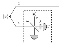
Figure 2: Quantum circuit describing our detector arrangement.

With this characterisation in mind, consider the circuit in figure 2. We have some multi-mode state $|\psi\rangle$ and we wish to condition the state of mode(s) $a$ dependent on a photon number measurement on mode $b$. For simplicity consider only a single $n$-photon Fock state component in mode $b$, the general case is recovered through additivity, i.e. $\mbox{$|\psi\rangle$}=\mathcal{N}_{0}\sum_{n}\mbox{$|\psi^{(n)}\rangle$}$. The input state is then some state $\mbox{$|\psi^{(n)}\rangle$}=\mbox{$|a_{n}\rangle$}_{a}\mbox{$|n\rangle$}_{b}\mbox{$|p\rangle$}_{c}$, where $|a_{n}\rangle$ is the associated component in mode $a$ and mode $c$ is initially in a $p$-photon Fock state. After interacting on a beam-splitter of reflectivity $\cos^{2}(\omega)$ and undergoing a phase shift $\lambda$ on mode $b$ the output state is

$$\mbox{$|\psi^{(n)}_{\mathrm{out}}\rangle$}= \frac{\mbox{$|a_{n}\rangle$}_{a}}{\sqrt{n!p!}}\sum_{m=0}^{n}\sum_{q=0}^{p}\binom{n}{m}\binom{p}{q}e^{i\pi(p-q)+i(m+q)\lambda}$$

$$\times c^{m+p-q}s^{n-m+q}\mbox{\boldmath$\hat{b}$}^{\dagger m+q}\mbox{\boldmath$\hat{c}$}^{\dagger n+p-(m+q)}\mbox{$|00\rangle$}_{bc}$$ (2)

where $\mbox{\boldmath$\hat{b}$}^{\dagger}$ and $\mbox{\boldmath$\hat{c}$}^{\dagger}$ are the bosonic creation operators for modes $b$ and $c$ respectively, $c=\cos(\omega)$, $s=\sin(\omega)$, and finally we also have the usual binomial coefficients $\binom{u}{v}=\frac{u!}{(u-v)!v!}$.

Modes $b$ and $c$ are now detected using separate balanced homodyne detectors. To an excellent approximation such detectors can be modeled as projectors onto small ranges of quadrature amplitude eigenstates $|x_{\theta}\rangle$ where $x_{\theta}$ is a continuous variable with infinite dimension, and $\theta$ describes the phase relationship with the local oscillator of the homodyne detector. The final conditional state (unnormalised), given we obtain $x_{\theta}$ in one detector and $y_{\phi}$ in the other, is $\mbox{$|\psi_{\mathrm{cond}}\rangle$}=\mathcal{N}_{0}\sum_{n}\mbox{$|x,y\rangle\langle x,y|$}\mbox{$|\psi^{(n)}_{\mathrm{out}}\rangle$}=\mathcal{N}_{0}\sum_{n}\mbox{$|\psi^{(n)}_{\mathrm{cond}}\rangle$}$ where,

$$\mbox{$|\psi^{(n)}_{\mathrm{cond}}\rangle$}= \frac{e^{-i(n+p)\phi-\frac{1}{2}(x_{\theta}^{2}+y_{\phi}^{2})}\mbox{$|a_{n},x_{\theta},y_{\phi}\rangle$}}{\sqrt{n!p!\pi 2^{n+p}}}$$

$$\times\sum_{m=0}^{n}\sum_{q=0}^{p}\binom{n}{m}\binom{p}{q}e^{i\pi(p-q)+i(m+q)(\lambda-\theta+\phi)}$$

$$\times c^{m+p-q}s^{n-m+q}H_{{m+q}}(x_{\theta})H_{{n+p-(m+q)}}(y_{\phi})$$ (3)

where we have used the fact that the overlap between the quadrature amplitude eigenstates and the number states is given by

$$\mbox{$\langle x_{\theta}|n\rangle$}=\frac{H_{n}(x_{\theta})}{\sqrt{\sqrt{\pi}2^{n}n!}}e^{-\frac{1}{2}x_{\theta}^{2}-in\theta}$$ (4)

and $H_{n}(x)$ is the Hermite polynomial of order $n$. We have chosen the convention that the $\theta=0$ quadrature operator can be written in terms of the mode operators as $X=(a+a^{\dagger})/\sqrt{2}$. Notice that the quadrature phase angles $\theta$ and $\phi$ are effectively not independent of $\lambda$ and that without loss of generality we can absorb those terms into $\lambda$ (so we will take $\lambda-\theta+\phi\rightarrow\lambda$). For simplicity we shall also take $\phi=0$ and set the overall phase of this component to zero, and hence we can also drop the quadrature angle subscript on $x$ and $y$. Now consider the case where we use a 50:50 beam-splitter so that $\omega=\pi/4$ and we set $\lambda=\pi/2$. With these conditions equation (3) reduces to

$$\mbox{$|\psi^{(n)}_{\mathrm{cond}}\rangle$}= \frac{e^{-\frac{1}{2}(x^{2}+y^{2})}e^{i\pi p}}{\sqrt{n!p!\pi}2^{n+p}}g(n,p)\mbox{$|a_{n},x,y\rangle$}$$ (5)

$$g(n,p)= \sum_{m=0}^{n}\sum_{q=0}^{p}\binom{n}{m}\binom{p}{q}e^{i\frac{\pi}{2}(m-q)}$$

$$\times H_{{m+q}}(x)H_{{n+p-(m+q)}}(y)$$ (6)

To see how this detecting scheme is only sensitive to the $p$-Fock component we focus on the limiting case of $\Delta=0$ next.

III Limiting Case

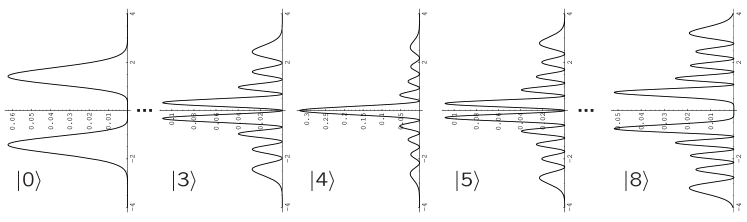
Figure 3: Probability density plots for obtaining a particular $x$ and $y$ for the homodyne detections given an auxiliary photon number of $\mbox{$|p\rangle$}=\mbox{$|4\rangle$}$, for various input number states $|n\rangle$. Only the $x$ axis shown as the distributions are rotationally symmetric. By post-selecting on a narrow band near $x=0$ the detector becomes only sensitive to components with $\mbox{$|n\rangle$}=\mbox{$|p\rangle$}$. Also, the noise form having a finite post-selection band comes from the nearby number states from the target state.

Consider only the special case where we happen to detect $x=y=0$ in the homodyne detectors. For these values, we can use

$$H_{n}(0)=\left\{\begin{array}[]{cl}0&n\;\mathrm{odd}\\ \frac{(-1)^{n/2}n!}{(n/2)!}&n\;\mathrm{even}\end{array}\right.$$ (7)

This relation implies that only terms with even $m+q$ will be non-zero, which in turn implies that $n+p$ must be even also. If we now write $g\rightarrow[g(n,p)+g^{\prime}(n,p)]/2$ where $g^{\prime}(n,p)$ simply has the order of the summations reversed, we get

$$g(n,p)=\frac{1}{2}\sum_{m=0}^{n}\sum_{q=0}^{p}\binom{n}{m}\binom{p}{q}H_{{m+q}}(0)H_{{n+p-(m+q)}}(0)$$

$$e^{i\frac{\pi}{2}(m-q)}\left(1+e^{i\pi k}\right)$$ (8)

where we have set $n=p+2k$ and used the fact that $m+q$ must be even. From this expression it is clear that terms with odd $k$ will also vanish. Terms with even $k>0$ will also vanish — this can be readily verified numerically. This then only leaves the terms with $k=0$ ($n=p$) as contributing to the state (5) and so the detector picks out the $|a_{p}\rangle$ component.

This analysis assumes an infinitesimal acceptance band for the detector. In order to assess the practicalities of the system we need to integrate over some range of values around $x=y=0$ and evaluate success and failure probabilities. Clearly there will be a tradeoff between how well we project onto the $p$-photon Fock state and the probability of obtaining a successful outcome.

IV Finite $\Delta$

The probability density for obtaining a value $x$ in mode $c$ and $y$ in mode $b$ will be

$$P(x,y) = \mathrm{tr}\{\mbox{$|x\rangle\langle x|$}\otimes\mbox{$|y\rangle\langle y|$}\rho\}$$ (9)

$$= \mathrm{tr}_{a}\{\mbox{$\langle x,y|$}\rho\mbox{$|x,y\rangle$}\}$$ (10)

where $\rho$ is the three mode density matrix describing the state after the beam-splitter. This distribution is radially symmetric about the origin, so we will switch to the polar co-ordinates $r$ and $\theta$ (where $r^{2}=x^{2}+y^{2}$) and accept a particular result if it lies within a certain radius $\Delta$. Intuitively we can see what the effect will be from figure 3. As we make $\Delta$ larger, the probability that a result falls within the accepted band, picks up contributions from nearby states to the target state, and these will contribute to the error. The total probability that we get $0\leq r\leq\Delta$ is

$$P_{\Delta}=2\pi\int_{0}^{\Delta}P(r,\theta)rdr$$ (11)

The (unnormalised) state immediately after destructively obtaining a particular $x$ and $y$ in the first two modes is $\rho^{(x,y)}_{a}=\mbox{$\langle x,y|$}\rho\mbox{$|x,y\rangle$}$. Consequently the ensemble of states that we would obtain if we where to only accept values within a radius $\Delta$, would be

$$\rho_{a}=\frac{1}{P_{\Delta}}\int_{0}^{2\pi}d\theta\int_{0}^{\Delta}dr\;\rho^{(r,\theta)}_{a}$$ (12)

Figure 4: The main source of error for the detector is due to contributions from number states near the target state. Here we plot the difference in fidelity $F$, between two successive window sizes, $w$ and $w+1$. As can be seen, increasing the size of the window of states we are testing against makes little difference past a few states, consequently we will adopt $w=2$ in calculations. Note that $\Delta=0.1$ in the plots.

To compare how well such a projector functions we can use the fidelity against the target state $|a_{p}\rangle$:

$$F(\Delta)=|\mbox{$\langle a_{p}|$}\rho_{a}\mbox{$|a_{p}\rangle$}|$$ (13)

Note that in calculating this quantity we will assume that the $|a_{j}\rangle$ are orthonormal.

One of the important features of the PAD scheme is that it is sensitive only to a band of number states near the target state. This effect can be seen in the behaviour of the probability densities for states far away from the target state in figure 3, and is clearly demonstrated in figure 4, where we show the rapid convergence in fidelity as we increase the number of nearby states to the one we are projecting out.

As we increase $\Delta$, the probability that we get a result we will accept also increases, but due to the overlap with the states near the target state the fidelity of the detector will drop. The actual probability is not a meaningful quantity in this context as it depends as much on the test state (1) as on the parameters of the detector. The quantity we will use instead is a probability rate $R=P_{\Delta}/P_{\mathrm{ideal}}$, which is the probability we get divided by the expected probability if we had an ideal photo-counter. The tradeoff between fidelity and probability is quantified in figure 5.

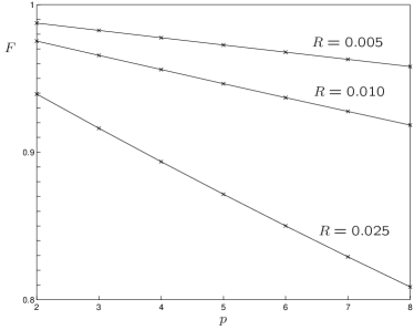
Figure 5: The fidelity of operation for various target states $|a_{p}\rangle$ from the distributions (1) is given (with $w=2$). The curves are for fixed probability rates $R$.

V Inefficient Detection

The calculations so far have assumed unit efficiency detection. In this section we explore the effect of non-unit detection efficiencies for the PAD, although it should be noted from the outset that detection efficiency for homodyne detection is very high (in the region of 98% 92polzik3020 ). We will compare the performance of the PAD to an ideal, but inefficient photon counter, which we model by the POVM elements $\Pi_{p}:p=0,1,\ldots$, where $p$ is the number of detected photons, with

$$\Pi_{p}=\sum_{m=p}^{\infty}\binom{m}{p}\eta^{p}(1-\eta)^{m-p}\mbox{$|m\rangle\langle m|$}$$ (14)

Visible-light photon counters can be modelled as ideal, but inefficient photon counters, at least for small photon numbers 0204073 .

The fidelity of the ideal detector in picking out the state $|a_{p}\rangle$ when used with the input state (1) is then

$$F_{\mathrm{ideal}} =\frac{|\mbox{$\langle a_{p}|$}\mathrm{Tr}_{b}\{\Pi_{p}\rho_{\mathrm{in}}\}\mbox{$|a_{p}\rangle$}|}{\mathrm{Tr}\{\Pi_{p}\rho_{\mathrm{in}}\}}$$

$$=\left(\sum_{n=p}^{n_{\mathrm{max}}}\binom{n}{p}(1-\eta)^{n-p}\right)^{-1}$$ (15)

where the summation extends to the maximum photon number, so for the test state in (1) $n_{\mathrm{max}}=p+w$.

For the PAD detector we can model inefficiencies simply by considering a beam splitter of transitivity $\eta$ in front of both homodyne detectors 93leonhardt4598 . The first observation we make is that for high efficiency, the ideal detector obtains a higher fidelity. The trend with higher photon number is similar for both detectors. Where the advantage lies for the PAD is that the efficiency for current homodyne detectors is very high compared with available photon counters.

For a particular $\Delta$ and $\eta$ we can consider an equivalent ideal detector that gives the same fidelity. Constructing an equivalence in this fashion is particularly useful and was considered by 02nemoto032306 where they compared an ideal photon counter with homodyne detection in the context of quantum communication. As such, they used the mutual information as a means of comparison. For our scheme, we envision state preparation as the main application so we will use the fidelity as a means of comparison. This comparison is plotted in figure 6, for the ability to project out the state $|a_{1}\rangle$ from the input state $\sum_{n=0}^{4}\mbox{$|a_{n}\rangle$}\mbox{$|n\rangle$}$. A detector able to achieve this projection forms a selective detector which is needed in many linear optics schemes.

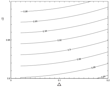
Figure 6: Equivalent ideal single photon detector efficiency as a function of the acceptance width $\Delta$, and the Homodyne efficiency $\eta$.

VI Discussion and Conclusions

Because of it’s non-deterministic nature, we envision applications of this detector mainly in state preparation, where non-classical states are prepared through conditioning on photon number detection. We could prepare a good approximation to an $|n\rangle$ photon state required by our detector, by using spontaneous parametric down conversion and a detector cascade in one arm. Even if the detectors in the cascade are inefficient, if, say three detectors register a click, then we have at least a three photon term in the other arm. The errors caused by having more than the required number of photons are offset by the low probability of such events. One intriguing possibility is to employ this detector in a proposal by Dakna, et al. 97dakna3184 . In the Dakna scheme, a good approximation to an optical Schrödinder cat state is generated by mixing a single mode squeezed state on a beam-splitter with the vacuum and conditioning on detecting a certain number of photons in one of the exit ports.

Another possible extension is to use other parameter choices, and post-selection choices to directly project out certain distributions of photon number terms.

We have presented a non-deterministic scheme which functions as a high-fidelity Fock state projector. This detecting scheme allows a tunable tradeoff between the fidelity and probability of detection. The weaknesses of the scheme are that it requires an $|n\rangle$ photon state and that it is non-deterministic. The $|n\rangle$ photon state could be prepared in the first instance simply by conditioning the output of a spontaneous parametric down converter with a traditional detector cascade. The non-deterministic nature of the scheme leads us to conclude that the main application for the detector will be in state generation.

AG acknowledges support form the New Zealand Foundation for Research, Science and Technology under grant UQSL0001. This project was supported by the Australian Research Council.

References

- (1) E. Knill, R. Laflamme, and G. Milburn, Nature 409, 46 (2001).
- (2) D. Gottesman and I. L. Chuang, Nature 402, 390 (1999).
- (3) T. B. Pittman, B. C. Jacobs, and J. D. Franson, Phys. Rev. A 64, 062311 (2001).
- (4) T. C. Ralph, A. G. White, W. J. Munro, and G. J. Milburn, Phys. Rev. A 65, 012314 (2002).
- (5) E. Knill, Phys. Rev. A 66, 052306 (2002).
- (6) T. C. Ralph, W. J. Munro, and G. J. Milburn, Quantum Computation with Coherent States, Linear Interactions and Superposed Resources, 2001, quant-ph/0110115.
- (7) H. Lee, P. Kok, N. J. Cerf, and J. P. Dowling, Phys. Rev. A 65, 030101(R) (2002).
- (8) P. Kok, H. Lee, and J. P. Dowling, Phys. Rev. A 65, 052104 (2002).
- (9) J. Fiurásek, Phys. Rev. A 65, 053818 (2002).
- (10) X. Zou, K. Pahlke, and W. Mathis, Phys. Rev. A 66, 014102 (2002).
- (11) J. Kim, S. Takeuchi, Y. Yamamoto, and H. H. Hogue, Appl. Phys. Lett. 74, 902 (1999).
- (12) S. Takeuchi, J. Kim, Y. Yamamoto, and H. H. Hogue, Appl. Phys. Lett. 74, 1063 (1999).
- (13) P. Kok and S. L. Braunstein, Phys. Rev. A 63, 033812 (2001).
- (14) E. S. Polzik, J. Carri, and H. J. Kimble, Phys. Rev. Lett. 68, 3020 (1992).
- (15) S. D. Bartlett, E. Diamanti, B. C. Sanders, and Y. Yamamoto, Photon counting schemes and performance of non-deterministic nonlinear gates in linear optics, quant-ph/0204073, proceedings of Free-Space Laser Communication and Laser Imaging II, Vol. 4821, SPIE International Symposium on Optical Science and Technology (7-11 July 2002), eds. J C Ricklin and D G Voelz (SPIE, Bellingham, WA, 2002).
- (16) U. Leonhardt and H. Paul, Phys. Rev. A 48, 4598 (1993).
- (17) K. Nemoto and S. L. Braunstein, Phys. Rev. A 66, 032306 (2002).
- (18) M. Dakna et al., Phys. Rev. A 55, 3184 (1997).