Multiorder coherent Raman scattering of a quantum probe field

Abstract

We study the multiorder coherent Raman scattering of a quantum probe field in a far-off-resonance medium with a prepared coherence. Under the conditions of negligible dispersion and limited bandwidth, we derive a Bessel-function solution for the sideband field operators. We analytically and numerically calculate various quantum statistical characteristics of the sideband fields. We show that the multiorder coherent Raman process can replicate the statistical properties of a single-mode quantum probe field into a broad comb of generated Raman sidebands. We also study the mixing and modulation of photon statistical properties in the case of two-mode input. We show that the prepared Raman coherence and the medium length can be used as control parameters to switch a sideband field from one type of photon statistics to another type, or from a non-squeezed state to a squeezed state and vice versa.

I Introduction

The parametric beating of a weak probe field with a prepared Raman coherence in a far-off-resonance medium has been extensively studied Liang ; Katsuragawa ; Nazarkin99 ; beating . It has been demonstrated that multimode laser radiation Liang and incoherent fluorescent light Katsuragawa can be replicated into Raman sidebands. Since a substantial molecular coherence can be produced by the two-color adiabatic Raman pumping method Modulation ; D2 ; subfem ; Kien99 , the quantum conversion efficiency of the parametric beating technique can be maintained high even for weak light with less than one photon per wave packet Katsuragawa . To describe the statistical properties of a weak quantum probe and its first-order Stokes and anti-Stokes sidebands in the parametric beating process, a simplified quantum treatment has recently been performed three sidebands . It has been shown that the statistical properties of the quantum probe can be replicated into the two sidebands nearest to the input line, in agreement with the experimental observations Liang ; Katsuragawa .

However, many experiments have reported the observations of ultrabroad Raman spectra with a large number of sidebands Liang ; Katsuragawa ; Nazarkin99 ; Modulation ; D2 . In the experiments with solid hydrogen Liang ; Katsuragawa , at least two anti-Stokes sidebands and two Stokes sidebands have been observed. In the experiment with molecular deuterium D2 , a large Raman coherence $|\rho_{ab}|\cong 0.33$ and about 20 Raman sidebands, covering a wide spectral range from near infrared through vacuum ultraviolet, have been generated. In rare-earth doped dielectrics with low Raman frequency and long-lived spin coherence, a substantial Raman coherence $|\rho_{ab}|\cong 0.25$ and an extremely large number of sidebands (about $10^{4}$) can also be generated kolesov . Broad combs of Raman sidebands Liang ; Katsuragawa ; Nazarkin99 ; Modulation ; D2 have been intensively studied because they may synthesize to subfemtosecond subfem ; Kien99 ; Sokolov01 ; korn02 and subcycle HarrisSeries pulses. The generation of broad combs of Raman sidebands has always been examined as a semiclassical problem. While classical treatments are sufficient for many purposes, a quantum treatment is required when the statistical properties of the radiation fields are important. On the other hand, broad combs of Raman sidebands with similar nonclassical properties and different frequencies may find useful applications for high-performance optical communication. Therefore, it is intriguing to examine the quantum aspects of high-order coherent Raman processes.

In this paper, we extend the treatment of Ref. three sidebands to study various quantum properties of multiorder sidebands generated by the beating of a quantum probe field with a prepared Raman coherence in a far-off-resonance medium. Under the conditions of negligible dispersion and limited bandwidth, we derive a Bessel-function solution for the sideband field operators. We analytically and numerically calculate various quantum statistical characteristics of the sideband fields generated from a single-mode quantum input. We show that, with increasing the effective medium length or the Raman sideband order, the autocorrelation functions, cross-correlation functions, photon-number distributions, and squeezing factors undergo oscillations governed by the Bessel functions. Meanwhile, the normalized autocorrelation functions and normalized squeezing factors of the single-mode probe field are not altered and can be replicated into a broad comb of generated multiorder Raman sidebands. We study the mixing and modulation of photon statistical properties in the case of two-mode input. We show that the prepared Raman coherence and the medium length can be used as control parameters to switch a sideband field from one type of photon statistics to another type, or from a non-squeezed state to a squeezed state and vice versa. We also discuss two-photon interference in coherent Raman scattering. Although the multiorder coherent Raman scattering can produce a broad comb of sideband fields with different frequencies, it behaves in many aspects as a beam splitter coupler ; Mandel and Scully book ; beam splitter ; Hong ; applications ; Knight . Therefore, in this paper, we also make comparison of this conventional device with our system as and when it is possible.

Before we proceed, we note that, in related problems, the generation of correlated photons using the $\chi^{(2)}$ and $\chi^{(3)}$ parametric processes has been studied Mandel and Scully book ; coupler ; Wang . The correlations between the Stokes and anti-Stokes sidebands and the possibility of transferring a quantum state of light from one carrier frequency to another carrier frequency (multiplexing) have been discussed for resonant systems Scully .

The paper is organized as follows. In Sec. II, we describe the model and present the basic equations. In Sec. III, we study various quantum characteristics of the sideband fields generated from a single-mode quantum input. In Sec. IV, we discuss the quantum properties of the sideband fields generated from a two-mode quantum input. Finally, we present the conclusions in Sec. V.

II Model

We consider a far-off-resonance Raman medium shown schematically in Fig. 1. Level $a$ with energy $\omega_{a}$ is coupled to level $b$ with energy $\omega_{b}$ by a Raman transition via intermediate levels that are not shown in the figure. We send a pair of long, strong, classical laser fields, with carrier frequencies $\omega_{-1}^{(d)}$ and $\omega_{0}^{(d)}$, and a short, weak, quantum probe field $\hat{E}_{\mathrm{in}}$, with one or several carrier frequencies, through the Raman medium, along the $z$ direction. The timing and alignment of these fields are such that they substantially overlap with each other during the interaction process. The driving laser fields are tuned close to the Raman transition $a\leftrightarrow b$, with a small finite two-photon detuning $\delta$, but are far detuned from the upper electronic states $j$ of the molecules. We assume that all the frequency components of the input probe field are separated by integer multiples of the Raman modulation frequency $\omega_{m}=\omega_{b}-\omega_{a}-\delta$. The driving fields adiabatically produce a Raman coherence $\rho_{ab}$ subfem ; Kien99 . When the probe field propagates through the medium, it beats with the prepared Raman coherence. Since the probe field is weak and short compared to the driving fields, the medium state and the driving fields do not change substantially during this step. The beating of the probe field with the prepared Raman coherence leads to the generation of new sidebands in the total output field $\hat{E}_{\mathrm{out}}$. The frequencies of the sideband fields $\hat{E}_{q}$ are given by $\omega_{q}=\omega_{0}+q\omega_{m}$, where $q$ is integer and $\omega_{0}$ is a carrier frequency of the input probe field. The range of $q$ should be appropriate so that $\omega_{q}$ is positive. The probe field is taken to be not too short so that the Fourier-transformation limited broadening is negligible. We assume that the prepared Raman coherence $\rho_{ab}$ is substantial so that the spontaneous Raman process is negligible compared to the stimulated and parametric processes. Consequently, the quantum noise can be neglected. Unlike Ref. three sidebands , our model does not require any restriction on the magnitude of the coherence as all Raman sidebands are included. When we take the propagation equation for the classical Raman sidebands subfem ; Kien99 and replace the field amplitudes by the quantum operators, we obtain

$$\frac{\partial\hat{E}_{q}}{\partial z}+\frac{\partial\hat{E}_{q}}{c\partial t}=i\beta_{q}(u_{q}\hat{E}_{q}+d_{q-1}\rho_{ba}\hat{E}_{q-1}+d_{q}\rho_{ab}\hat{E}_{q+1}).$$ (1)

Here, $u_{q}$ and $d_{q}$ are the dispersion and coupling constants, respectively. We have denoted $\beta_{q}={\cal N}\hbar\omega_{q}/\epsilon_{0}c$, where ${\cal N}$ is the molecular number density.

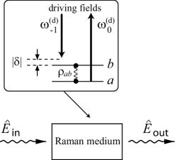
Figure 1: Principle of the technique: Two classical laser fields drive a Raman transition of molecules in a far-off-resonance medium. The beating of a weak quantum probe field with the prepared Raman coherence produces new sideband fields.

We take all the sidebands to be sufficiently far from resonance that the dispersion of the medium is negligible. In this case, we have $u_{q}=u_{0}$ and $d_{q}=d_{0}$. We write $\rho_{ab}=\rho_{0}\exp[i(\phi_{0}-\beta_{m}u_{0}z)]$, where $\rho_{0}\equiv|\rho_{ab}|$ and $\beta_{m}={\cal N}\hbar\omega_{m}/\epsilon_{0}c$, and assume that $\rho_{0}$ and $\phi_{0}$ are constant in time and space. We change the variables by $\hat{E}_{q}=\hat{\cal E}_{q}\exp[i(\beta_{q}u_{0}z-q\phi_{0})]$. Using photon operators, we can write $\hat{\cal E}_{q}(z,t)=(2\hbar\omega_{q}/\epsilon_{0}LA)^{1/2}\sum_{K}\hat{b}_{q}(K,t)e^{iK(z-ct)}$. Here, $L$ is the quantization length taken to be equal to the medium length, $A$ is the quantization transverse area taken to be equal to the beam area, $K$ is a Bloch wave vector, and $\hat{b}_{q}(K,t)$ and $\hat{b}_{q}^{\dagger}(K,t)$ are the annihilation and creation operators for photons in the spectral mode $q$ and the spatial mode $K$. For simplicity, we restrict our discussion to the case where each sideband field contains only a single spatial mode (with, e.g., $K=0$). Then, Eq. (1) yields

$$\frac{\partial\hat{b}_{q}}{\partial t}=i(g_{q}\hat{b}_{q-1}+g_{q+1}\hat{b}_{q+1}),$$ (2)

where $g_{q}=({\cal N}\hbar/\epsilon_{0})\sqrt{\omega_{q}\omega_{q-1}}\,d_{0}\rho_{0}$. For the medium length $L$, the evolution time is $t=L/c$. It follows from Eq. (2) that the total photon number is conserved in time. Note that Eq. (2) represents the Heisenberg equation for the fields that are coupled to each other by the effective interaction Hamiltonian

$$\hat{H}=-\hbar\sum_{q}g_{q+1}(\hat{b}_{q}\hat{b}_{q+1}^{\dagger}+\hat{b}_{q+1}\hat{b}_{q}^{\dagger}).$$ (3)

The interaction between the sideband fields via the prepared Raman coherence is analogous to the interaction between the transmitted and reflected fields from a conventional beam splitter Mandel and Scully book . However, the two mechanisms are very different in physical nature. The most important difference between them is that the two fields from the conventional beam splitter have the same frequency while the sideband fields in the Raman scheme have different frequencies. In addition, the model Hamiltonian (3) involves an infinitely large number of Raman sidebands, separated by integer multiples of the Raman modulation frequency $\omega_{m}$. Despite these differences, the model (3) can be called the multiorder Raman beam splitter. The parameters $g_{q}t=g_{q}L/c$ determine the transmission and scattering coefficients for the fields at the Raman beam splitter.

We assume that the bandwidth of the generated Raman spectrum is small compared to the characteristic probe frequency $\omega_{0}$. In this case, the $q$-dependence of the coupling parameters $g_{q}$ can be neglected, that is, we have $g_{q}=g_{0}={\cal N}\hbar\omega_{0}d_{0}\rho_{0}/\epsilon_{0}$. With this assumption, we find the following solution to Eq. (2):

$$\hat{b}_{q}(t)=\sum_{q^{\prime}}e^{i(q-q^{\prime})\pi/2}J_{q-q^{\prime}}(2g_{0}t)\hat{b}_{q^{\prime}}(0).$$ (4)

Here, $J_{k}$ is the $k$th-order Bessel function. The expression (4) for the output field operators is a generalization of the Bessel-function solution obtained earlier for the classical fields subfem ; Kien99 . The number of generated Raman sidebands is characterized by the effective interaction time $2g_{0}t$ or, equivalently, the effective medium length $\kappa L$, where

$$\kappa=\frac{2g_{0}}{c}=\frac{2\hbar}{\epsilon_{0}c}{\cal N}\omega_{0}d_{0}\rho_{0}.$$ (5)

The coefficient $\kappa$ characterizes the strength of the parametric coupling and is proportional to the prepared Raman coherence $\rho_{0}$, that is, to the intensities of the driving laser fields. The Bessel functions $J_{k}(\kappa L)$ are the transmission ($k=0$) and scattering ($k\not=0$) coefficients for the Raman sidebands, similar to the transmission and reflection coefficients of a conventional beam splitter. The assumption of limited bandwidth requires $\kappa L\ll\omega_{0}/\omega_{m}$, that is, $(2\hbar/\epsilon_{0}c){\cal N}\omega_{m}d_{0}\rho_{0}L\ll 1$ subfem ; Kien99 . In what follows we use the expression (4) to calculate various quantum statistical characteristics of the sideband fields, namely, the autocorrelation functions, the two-mode cross-correlation functions, the squeezing factors, and the relation between the $P$ representations of the output and input states.

III Single-mode quantum input

In this section, we consider the case where the input probe field has a single carrier frequency $\omega_{0}$. In other words, we assume that the sideband $q=0$ is initially prepared in a quantum state $\hat{\rho}_{\mathrm{in}}^{(0)}$ and the other sidebands are initially in the vacuum state. The density matrix of the initial state of the fields is given by

$$\hat{\rho}_{\mathrm{in}}=\hat{\rho}_{\mathrm{in}}^{(0)}\otimes\prod_{q\not=0}(|0\rangle\langle 0|)_{q}.$$ (6)

III.1 Autocorrelation functions

We study the autocorrelations of photons in the generated Raman sidebands. We use Eq. (4) and apply the initial density matrix (6) to calculate the normally ordered moments $\langle\hat{b}_{q}^{\dagger n}\hat{b}_{q}^{n}\rangle$ of the photon-number operators $\hat{n}_{q}=\hat{b}_{q}^{\dagger}\hat{b}_{q}$. The result is

$$\langle\hat{b}_{q}^{\dagger n}\hat{b}_{q}^{n}\rangle=J_{q}^{2n}(\kappa L)\langle\hat{b}_{0}^{\dagger n}(0)\hat{b}_{0}^{n}(0)\rangle.$$ (7)

In particular, the mean photon numbers of the sidebands are given by

$$\langle\hat{n}_{q}\rangle=J_{q}^{2}(\kappa L)\langle\hat{n}_{\mathrm{in}}\rangle.$$ (8)

Here, $\hat{n}_{\mathrm{in}}=\hat{b}_{0}^{\dagger}(0)\hat{b}_{0}(0)$ is the photon-number operator for the input field. The $n$th-order autocorrelation functions of the sidebands are defined by $\Gamma_{q}^{(n)}=\langle\hat{b}_{q}^{\dagger n}\hat{b}_{q}^{n}\rangle-\langle\hat{b}_{q}^{\dagger}\hat{b}_{q}\rangle^{n}$. From Eqs. (7) and (8), we find

$$\Gamma_{q}^{(n)}=J_{q}^{2n}(\kappa L)\Gamma_{\mathrm{in}}^{(n)},$$ (9)

where $\Gamma_{\mathrm{in}}^{(n)}=\langle\hat{b}_{0}^{\dagger n}(0)\hat{b}_{0}^{n}(0)\rangle-\langle\hat{b}_{0}^{\dagger}(0)\hat{b}_{0}(0)\rangle^{n}$ is the $n$th-order autocorrelation function of the input field.

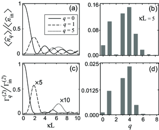
Figure 2: Mean photon number $\langle\hat{n}_{q}\rangle$ (first row) and second-order autocorrelation function $\Gamma_{q}^{(2)}$ (second row), both scaled to their initial values for the probe field, as functions of the effective medium length $\kappa L$ (first column) and the sideband order $q$ (second column). In (a) and (c), the sideband order is $0$ (solid line), $1$ (dashed line), and $5$ (dotted line). In (b) and (d), the effective medium length is $\kappa L=5$. In (c), we have amplified $\Gamma_{1}^{(2)}/\Gamma_{\mathrm{in}}^{(2)}$ (dashed line) and $\Gamma_{5}^{(2)}/\Gamma_{\mathrm{in}}^{(2)}$ (dotted line) by 5 and 10 times, respectively. In (b) and (d), the negative side of the $q$ axis is not shown because the functions plotted are symmetric in $q$.

Equations (8) and (9) indicate that, when we increase the effective medium length $\kappa L$ or the sideband order $q$, the mean photon number $\langle\hat{n}_{q}\rangle$ and the autocorrelation function $\Gamma_{q}^{(n)}$ undergo oscillations as described by even powers of the Bessel function $J_{q}(\kappa L)$. Such oscillatory behavior is illustrated in Fig. 2. When the sideband order $q$ is higher, the onset of $\langle\hat{n}_{q}\rangle$ occurs later [see Fig. 2(a)] and, hence, so does the onset of $\Gamma_{q}^{(n)}$ [see Fig. 2(c)]. For a fixed $q$, both $\langle\hat{n}_{q}\rangle$ and $\Gamma_{q}^{(n)}$ reach their largest values at the same optimal medium length $L_{q}=x_{q}/\kappa$, where $x_{q}$ is the position of the first peak of $J_{q}(x)$. The higher the sideband order $q$, the larger is the optimal length $L_{q}$ and the smaller are the maximal output values of $\langle\hat{n}_{q}\rangle$ and $\Gamma_{q}^{(n)}$ [see Figs. 2(a) and 2(c)]. Figures 2(b) and 2(d) show that $\langle\hat{n}_{q}\rangle$ and $\Gamma_{q}^{(n)}$ are substantially different from zero only in the region where $|q|$ is not too large compared to $\kappa L$. For a given $\kappa L$, both $\langle\hat{n}_{q}\rangle$ and $\Gamma_{q}^{(n)}$ achieve their maximal values at $q\approx\kappa L$.

The normalized $n$th-order autocorrelation functions of the sidebands are defined by $g_{q}^{(n)}=\langle\hat{b}_{q}^{\dagger n}\hat{b}_{q}^{n}\rangle/\langle\hat{b}_{q}^{\dagger}\hat{b}_{q}\rangle^{n}$. These functions characterize the overall statistical properties, such as sub-Poissonian, Poissonian, or super-Poissonian photon statistics, regardless of the mean photon number. Unlike the mean photon number $\langle\hat{n}_{q}\rangle$ and the autocorrelation function $\Gamma_{q}^{(n)}$, the normalized autocorrelation function $g_{q}^{(n)}$ does not oscillate when we change the effective medium length $\kappa L$ or the sideband order $q$. Indeed, with the help of Eq. (7), we find

$$g_{q}^{(n)}=g_{\mathrm{in}}^{(n)},$$ (10)

where $g_{\mathrm{in}}^{(n)}=\langle\hat{b}_{0}^{\dagger n}(0)\hat{b}_{0}^{n}(0)\rangle/\langle\hat{b}_{0}^{\dagger}(0)\hat{b}_{0}(0)\rangle^{n}$.

Equation (10) indicates that the generated sideband fields and the probe field have the same normalized autocorrelation functions, which are independent of the evolution time and are solely determined by the statistical properties of the input field. In other words, the normalized autocorrelation functions of the probe field do not change during the parametric beating process and are precisely replicated into the comb of generated sidebands. Such a replication of the normalized autocorrelation characteristics can be called autocorrelation multiplexing. In particular, if the photon statistics of the input field is sub-Poissonian, Poissonian, or super-Poissonian, the photon statistics of each of the sideband fields will also be sub-Poissonian, Poissonian, or super-Poissonian, respectively. This result is in agreement with the experiments on replication of multimode laser radiation Liang and broadband incoherent light Katsuragawa . The ability of the Raman medium to multiplex the autocorrelation characteristics is similar to the ability of a conventional beam splitter Mandel and Scully book .

It is not surprising that the normalized autocorrelation functions of the probe field are replicated into the sidebands in the parametric beating process. Such a replication is possible because the medium is far off resonance and the quantum probe field is weak compared to the driving fields. Under these two conditions, the photon annihilation operators are linearly transformed as described by the linear differential equation (2). This equation shows that the photon annihilation operators are not mixed up with the creation operators, and therefore the evolution of the annihilation operators is linear with respect to the initial annihilation operators.

We should, however, emphasize here that the replication of all of the normalized autocorrelation functions $g_{\mathrm{in}}^{(n)}$ (for all orders $n$) of the input field does not mean the replication of the quantum state $\hat{\rho}_{\mathrm{in}}^{(0)}$. In fact, the oscillations of the mean photon number $\langle\hat{n}_{q}\rangle$ and the autocorrelation function $\Gamma_{q}^{(n)}$ indicate that the photon-number distributions and consequently the quantum states of the sidebands evolve in a rather complicated way and are quite different from those for the input field. A separable state at the input can produce an entangled state three sidebands ; entang . In addition, cross-correlations between the sidebands can be generated from initially uncorrelated fields, and a Fock state at the input does not produce sideband fields in isolated Fock states [see below].

III.2 Cross-correlation functions

We study the correlations between the generated Raman sidebands. For two different sidebands $k$ and $l$ ($k\not=l$), we have

$$\langle\hat{n}_{k}\hat{n}_{l}\rangle=J_{k}^{2}(\kappa L)J_{l}^{2}(\kappa L)\langle\hat{n}_{\mathrm{in}}(\hat{n}_{\mathrm{in}}-1)\rangle.$$ (11)

The cross-correlation function for the two sidebands is defined by $\Gamma_{kl}^{(2)}=\langle\hat{n}_{k}\hat{n}_{l}\rangle-\langle\hat{n}_{k}\rangle\langle\hat{n}_{l}\rangle$. Using Eqs. (8) and (11), we find

$$\Gamma_{kl}^{(2)}=J_{k}^{2}(\kappa L)J_{l}^{2}(\kappa L)\Gamma_{\mathrm{in}}^{(2)}.$$ (12)

When we extend $\Gamma_{kl}^{(2)}$ for $k=l$, we have $\Gamma_{kk}^{(2)}=\Gamma_{k}^{(2)}$. According to Eq. (12), the cross-correlation function $\Gamma_{kl}^{(2)}$ oscillates when we change the effective medium length $\kappa L$ or the sideband orders $k$ and $l$. Such oscillatory behavior is illustrated in Fig. 3.

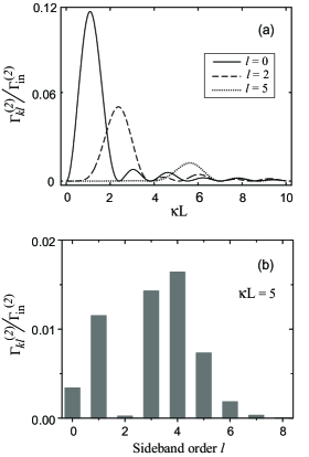
Figure 3: Cross-correlation function $\Gamma_{kl}^{(2)}$, scaled with the second-order autocorrelation function of the input field, as a function of (a) the effective medium length $\kappa L$ and (b) the sideband order $l$. Here, the sideband order $k$ is fixed to $1$. In (a), the sideband order $l$ is $0$ (solid line), $2$ (dashed line), and $5$ (dotted line). In (b), the effective medium length is $\kappa L=5$. In (b), the negative side of the $l$ axis is not shown because the function plotted is symmetric with respect to the sideband orders.

The normalized cross-correlation function is defined by $g_{kl}^{(2)}=\langle\hat{n}_{k}\hat{n}_{l}\rangle/(\langle\hat{n}_{k}\rangle\langle\hat{n}_{l}\rangle)$. Unlike the function $\Gamma_{kl}^{(2)}$, the normalized function $g_{kl}^{(2)}$ does not oscillate. Indeed, we find the relation

$$g_{kl}^{(2)}=g_{q}^{(2)}=g_{\mathrm{in}}^{(2)}.$$ (13)

As seen from the above relation, the normalized cross-correlation functions $g_{kl}^{(2)}$ for all possible sideband pairs $(k,l)$ are equal to each other, to the normalized second-order autocorrelation function $g_{q}^{(2)}$ for each sideband $q$, and to the normalized second-order autocorrelation function $g_{\mathrm{in}}^{(2)}$ of the input field. When $g_{\mathrm{in}}^{(2)}\not=1$, that is, when the photon statistics of the input field is non-Poissonian, we obtain $g_{kl}^{(2)}\not=1$, a signature of cross-correlations between the sidebands. Such correlations are generated although the sidebands are initially not correlated. In particular, if the input field has a sub-Poissonian photon statistics ($g_{\mathrm{in}}^{(2)}<1$), anti-correlations between the sidebands ($g_{kl}^{(2)}<1$) will be generated. Note that the conventional beam splitters also have a similar property Mandel and Scully book . The generation of cross-correlations between the sidebands indicates that the quantum states of the generated sidebands are different from that of the input field. We emphasize that the anti-correlation generation cannot be explained by the classical statistics of the fields with positive $P$ functions although the sideband dynamics is linear with respect to the field variables.

III.3 Photon-number distributions

To get deeper insight into the quantum properties of the generated Raman sidebands, we derive the photon-number distributions for the output fields. The joint photon-number distribution for the output fields is defined by $P_{\Sigma}(\{n_{q}\})=\langle\{n_{q}\}|\hat{\rho}_{\mathrm{out}}|\{n_{q}\}\rangle$, where $\hat{\rho}_{\mathrm{out}}=\hat{U}(L/c)\hat{\rho}_{\mathrm{in}}\hat{U}^{\dagger}(L/c)$ is the density matrix of the output state. Here, $\hat{U}(L/c)=\exp(-i\hat{H}L/\hbar c)$ is the evolution operator. Using Eqs. (4) and (6), we find

$$P_{\Sigma}(\{n_{q}\})=p_{\mathrm{in}}(N)\frac{N!}{\prod_{q}n_{q}!}\prod_{q}J_{q}^{2n_{q}}(\kappa L),$$ (14)

where $p_{\mathrm{in}}(n)=\mbox{}_{0}\langle n|\hat{\rho}_{\mathrm{in}}^{(0)}|n\rangle_{0}$ is the photon-number distribution of the input field, and $N=\sum_{q}n_{q}$ is the total photon number. From Eq. (14), the marginal photon-number distribution $p_{q}(n)$ for the sideband $q$ is obtained as

$$p_{q}(n)=\frac{J_{q}^{2n}(\kappa L)}{n!}\sum_{k=0}^{\infty}\frac{(n+k)!}{k!}[1-J_{q}^{2}(\kappa L)]^{k}p_{\mathrm{in}}(n+k).$$ (15)

Clearly, $p_{q}(n)$ is in general different from $p_{\mathrm{in}}(n)$. Thus, despite the replication of the normalized autocorrelation functions, the photon-number distribution of the probe field is not replicated into the sidebands.

We examine several particular cases. First, we consider the case where the probe field is initially prepared in a coherent state $|\alpha\rangle_{0}$. This state is characterized by a Poisson distribution $p_{\mathrm{in}}(n)=e^{-\bar{N}}\bar{N}^{n}/n!$ for the photon number, where $\bar{N}=|\alpha|^{2}$. In this case, Eqs. (14) and (15) yield $P_{\Sigma}(\{n_{q}\})=\prod_{q}p_{q}(n_{q})$ and

$$p_{q}(n)=e^{-\bar{n}_{q}}\frac{\bar{n}_{q}^{n}}{n!},$$ (16)

respectively, where $\bar{n}_{q}=\bar{N}J_{q}^{2}(\kappa L)$. Thus, the generated sidebands are not correlated, and the marginal photon-number distributions for the individual sidebands remain Poisson distributions during the evolution process.

Second, we consider the case where the probe field is initially in a Fock state $|N\rangle_{0}$. In this case, we have $p_{\mathrm{in}}(n)=\delta_{n,N}$. Therefore, Eq. (15) yields

$$p_{q}(n)=J_{q}^{2n}(\kappa L)[1-J_{q}^{2}(\kappa L)]^{N-n}\frac{N!}{n!(N-n)!}$$ (17)

for $n\leq N$, and $p_{q}(n)=0$ for $n>N$. Meanwhile, Eq. (14) yields $P_{\Sigma}(\{n_{q}\})\not=\prod_{q}p_{q}(n_{q})$, that is, the joint photon-number distribution is not a product of the marginal photon-number distributions for the individual sidebands. Thus, the sidebands are correlated. They are not generated in isolated Fock states.

Finally, we consider the case where the probe field is initially in a thermal state, which is characterized by a Boltzmann photon-number distribution $p_{\mathrm{in}}(n)=\bar{N}^{n}/(\bar{N}+1)^{n+1}$. In this case, Eq. (15) yields

$$p_{q}(n)=\frac{\bar{n}_{q}^{n}}{(\bar{n}_{q}+1)^{n+1}},$$ (18)

where $\bar{n}_{q}=\bar{N}J_{q}^{2}(\kappa L)$. Thus, the marginal photon-number distributions for the individual sidebands remain Boltzmann distributions during the evolution process. However, according to Eq. (14), we have $P_{\Sigma}(\{n_{q}\})\not=\prod_{q}p_{q}(n_{q})$, a signature of correlations between the generated sidebands.

III.4 Squeezing

We examine the squeezing of the field quadratures. A field quadrature of the $q$th mode is defined by $\hat{X}_{q}=\hat{b}_{q}^{\dagger}e^{i\varphi}+\hat{b}_{q}e^{-i\varphi}$. We say that the $q$th mode is in a squeezed state if there exists such a phase $\varphi$ that $\langle(\Delta\hat{X}_{q})^{2}\rangle<1$ or, equivalently, $S_{q}<0$, where $S_{q}=\langle(\Delta\hat{X}_{q})^{2}\rangle-1$. The squeezing degree is measured by the quantity $-S_{q}$. Note that the relation between the squeezing factor $S_{q}$ and the conventional squeezing parameter $r_{q}$ is $S_{q}=e^{-2r_{q}}-1$. In terms of the photon operators, we have

$$S_{q}=2[\langle\hat{b}_{q}^{\dagger}\hat{b}_{q}\rangle-\langle\hat{b}_{q}^{\dagger}\rangle\langle\hat{b}_{q}\rangle]+[(\langle\hat{b}_{q}^{2}\rangle-\langle\hat{b}_{q}\rangle^{2})e^{-2i\varphi}+\mathrm{c.c.}].$$ (19)

Using Eqs. (4) and (6), we find

$$\langle\hat{b}_{q}\rangle=e^{iq\pi/2}J_{q}(\kappa L)\langle\hat{b}_{0}(0)\rangle$$ (20)

and

$$\langle\hat{b}_{q}^{2}\rangle=e^{iq\pi}J_{q}^{2}(\kappa L)\langle\hat{b}_{0}^{2}(0)\rangle.$$ (21)

When we insert Eqs. (8), (20), and (21) into Eq. (19), we obtain

$$S_{q}(\varphi+q\pi/2)=J_{q}^{2}(\kappa L)S_{\mathrm{in}}(\varphi).$$ (22)

Here, $S_{\mathrm{in}}(\varphi)$ denotes the squeezing factor for the $\varphi$-quadrature of the input field. Equation (22) shows that, if $S_{\mathrm{in}}(\varphi)<0$, then $S_{q}(\varphi+q\pi/2)<0$. Thus, if the input field is in a squeezed state, then the generated sidebands are also in squeezed states. In other words, the squeezing of the input field is transferred to the comb of generated sidebands during the parametric beating process. The squeezing factor $S_{q}(\varphi+q\pi/2)$ of the sideband $q$ is reduced from the input squeezing factor $S_{\mathrm{in}}(\varphi)$ by the factor $J_{q}^{2}(\kappa L)$. Unlike the case of linear directional couplers and beam splitters coupler , the squeezing degree of the probe field cannot be completely transferred to the Raman sidebands. This difference is due to the fact that the linear directional coupler and the beam splitter involve only two output modes while the multiorder coherent Raman process involves many more output modes. Note that the phase of the squeezed quadrature of the sideband $q$ changes by $q\pi/2$. This means that the squeezed quadrature of a generated even-order (odd-order) Raman sideband is parallel (orthogonal) to that of the input field.

We introduce the normalized squeezing factor $s_{q}=S_{q}/\langle\hat{n}_{q}\rangle$. We find the relation

$$s_{q}(\varphi+q\pi/2)=s_{\mathrm{in}}(\varphi),$$ (23)

where $s_{\mathrm{in}}(\varphi)=S_{\mathrm{in}}(\varphi)/\langle\hat{n}_{\mathrm{in}}\rangle$ is the normalized squeezing factor for the input field. Equation (23) implies that, besides a shift of the quadrature phase angle, the normalized squeezing factor for the input field is replicated into the comb of generated sidebands. This result can be used to convert squeezing to a new frequency, i.e., to perform squeezing multiplexing. The relation $S_{q}(\varphi+q\pi/2)/S_{\mathrm{in}}(\varphi)=\langle\hat{n}_{q}\rangle/\langle\hat{n}_{\mathrm{in}}\rangle$ indicates that the $\kappa L$- and $q$-dependences of the squeezing factor $S_{q}(\varphi+q\pi/2)$ are similar to those of the mean photon number $\langle\hat{n}_{q}\rangle$ [see Figs. 2(a) and 2(b)]. Note that, when the input field is in a coherent state, the sideband fields have no squeezing. This property is similar to the case of four-wave mixing but is unlike the case of degenerate parametric down-conversion, where perfect squeezing can in principle be obtained. Since squeezed states are nonclassical states, the ability of the Raman medium to multiplex squeezing from a probe field to its sidebands is a quantum property that cannot be described by the classical statistics of the fields with positive $P$ functions.

III.5 Quantum states of the output fields

We calculate the quantum state of the output fields for several cases. First, we consider the case where the input sideband $0$ is initially in a coherent state $|\alpha\rangle_{0}$. The state of the fields at the input is

$$|\Psi_{\mathrm{in}}\rangle=|\alpha\rangle_{0}\prod_{q\not=0}|0\rangle_{q}=e^{-|\alpha|^{2}/2}e^{\alpha\hat{b}_{0}^{\dagger}(0)}|0\rangle.$$ (24)

The state of the fields at the output is given by $|\Psi_{\mathrm{out}}\rangle=\hat{U}(L/c)|\Psi_{\mathrm{in}}\rangle$. Since $\hat{U}(L/c)|0\rangle=|0\rangle$, we have $|\Psi_{\mathrm{out}}\rangle=e^{-|\alpha|^{2}/2}e^{\alpha\hat{b}_{0}^{\dagger}(-L/c)}|0\rangle$. Using Eq. (4), we find

$$|\Psi_{\mathrm{out}}\rangle=|\{\alpha_{q}(L/c)\}\rangle\equiv\prod_{q}|\alpha_{q}(L/c)\rangle_{q}.$$ (25)

Here, $|\alpha_{q}(L/c)\rangle_{q}$ is a coherent state of the $q$th mode, with the amplitude

$$\alpha_{q}(L/c)=\alpha J_{q}(\kappa L)e^{iq\pi/2}.$$ (26)

Thus, a probe field in a coherent state can produce sideband fields that are also in coherent states. Such a process can be called coherent-state multiplexing. This property of the Raman medium is similar to the case of conventional beam splitters Mandel and Scully book .

Second, we consider the case where the input sideband $0$ is initially prepared in a Fock state $|N\rangle_{0}$. The state of the fields at the input is written as

$$|\Psi_{\mathrm{in}}\rangle=|N\rangle_{0}\prod_{q\not=0}|0\rangle_{q}=\frac{1}{\sqrt{N!}}\hat{b}_{0}^{\dagger N}(0)|0\rangle.$$ (27)

The output state of the fields is given by $|\Psi_{\mathrm{out}}\rangle=(N!)^{-1/2}\hat{b}_{0}^{\dagger N}(-L/c)|0\rangle$. With the help of Eq. (4), we find

$$|\Psi_{\mathrm{out}}\rangle=\sum_{\{n_{q}\}}C_{\{n_{q}\}}^{(N)}|\{n_{q}\}\rangle.$$ (28)

Here,

$$C_{\{n_{q}\}}^{(N)}=\sqrt{\frac{N!}{\prod_{q}n_{q}!}}\prod_{q}e^{iqn_{q}\pi/2}J_{q}^{n_{q}}(\kappa L)$$ (29)

for $\sum_{q}n_{q}=N$, and $C_{\{n_{q}\}}^{(N)}=0$ for $\sum_{q}n_{q}\not=N$. When $N\not=0$ and $\kappa L\not=0$, the output state (28) is, in general, a multipartite inseparable (entangled) state.

In a particular case where the input state of the probe field is a single-photon state, i.e., $N=1$, Eqs. (28) and (29) yield

$$|\Psi_{\mathrm{out}}\rangle=\sum_{q}e^{iq\pi/2}J_{q}(\kappa L)|1_{q}\rangle.$$ (30)

Here, $|1_{q}\rangle$ is the quantum state of a single photon in the sideband $q$ with no photons in the other sidebands. In this case, the entanglement between two different sidebands $k$ and $l$ at the output can be measured by the bipartite concurrence $C_{kl}=2|J_{k}(\kappa L)J_{l}(\kappa L)|$, see entang .

Finally, we consider the case where the input sideband $0$ is initially in an incoherent mixed state

$$\hat{\rho}_{\mathrm{in}}^{(0)}=\sum_{n}p_{\mathrm{in}}(n)(|n\rangle\langle n|)_{0}.$$ (31)

With the help of Eq. (28), the density matrix of the output state of the fields is found to be

$$\hat{\rho}_{\mathrm{out}}=\sum_{N,\{n_{q}\},\{n^{\prime}_{q}\}}p_{\mathrm{in}}(N)C_{\{n_{q}\}}^{(N)}C_{\{n^{\prime}_{q}\}}^{(N)*}|\{n_{q}\}\rangle\langle\{n^{\prime}_{q}\}|.$$ (32)

To obtain the reduced density matrix $\hat{\rho}_{\mathrm{out}}^{(q)}$ for an arbitrary sideband $q$, we trace the total density matrix (32) over all sidebands except for the sideband $q$. Then, we find

$$\hat{\rho}_{\mathrm{out}}^{(q)}=\sum_{n}p_{q}(n)(|n\rangle\langle n|)_{q},$$ (33)

where the marginal photon-number distribution $p_{q}(n)$ is given by Eq. (15). As seen, the reduced state of each sideband is also an incoherent superposition of Fock states. However, if the input state is different from the vacuum state, then, for $\kappa L\not=0$, we have $\hat{\rho}_{\mathrm{out}}\not=\prod_{q}\hat{\rho}_{\mathrm{out}}^{(q)}$, a signature of correlations between the generated sidebands. Moreover, the total density matrix (32) of the output fields contains nonzero off-diagonal matrix elements in the Fock-state basis.

In a particular case where the initial state of the probe field is a thermal state, i.e., $\hat{\rho}_{\mathrm{in}}^{(0)}=\sum_{n}[\bar{N}^{n}/(\bar{N}+1)^{n+1}](|n\rangle\langle n|)_{0}$, the reduced state of each generated sideband is also a thermal state, namely,

$$\hat{\rho}_{\mathrm{out}}^{(q)}=\sum_{n}\frac{\bar{n}_{q}^{n}}{(\bar{n}_{q}+1)^{n+1}}(|n\rangle\langle n|)_{q}.$$ (34)

Here, $\bar{n}_{q}=\bar{N}J_{q}^{2}(\kappa L)$ is the mean photon number for the sideband $q$. The reduced thermal states of the generated sidebands are, however, not isolated from each other.

IV Two-mode quantum input

A far-off-resonance medium with a substantial Raman coherence, prepared by two strong driving fields, can efficiently mix and modulate the quantum statistical properties of the sideband fields. To understand this mechanism, we study the case where the input probe field has two carrier frequencies, $\omega_{0}$ and $\omega_{\nu}=\omega_{0}+\nu\omega_{m}$, separated by an integer multiple $\nu$ of the Raman modulation frequency $\omega_{m}$. We assume that the Raman sidebands $0$ and $\nu$ are initially in independent quantum states $\hat{\rho}_{\mathrm{in}}^{(0)}$ and $\hat{\rho}_{\mathrm{in}}^{(\nu)}$, respectively, while the other sidebands are initially in the vacuum state. The density matrix of the initial state of the fields is given by

$$\hat{\rho}_{\mathrm{in}}=\hat{\rho}_{\mathrm{in}}^{(0)}\otimes\hat{\rho}_{\mathrm{in}}^{(\nu)}\otimes\prod_{q\not=0,\nu}(|0\rangle\langle 0|)_{q}.$$ (35)

Here, $\nu\not=0$.

IV.1 Modulation of photon statistics

We study the mixing and modulation of photon statistics of the sideband fields. When we use Eq. (4) to calculate the mean photon numbers of the sidebands generated from the initial state (35), we find

$$\langle\hat{b}_{q}^{\dagger}\hat{b}_{q}\rangle = J_{q}^{2}(\kappa L)\langle\hat{b}_{0}^{\dagger}(0)\hat{b}_{0}(0)\rangle+J_{q-\nu}^{2}(\kappa L)\langle\hat{b}_{\nu}^{\dagger}(0)\hat{b}_{\nu}(0)\rangle$$ (36)

$$\mbox{}+J_{q}(\kappa L)J_{q-\nu}(\kappa L)$$

$$\mbox{}\times[e^{-i\nu\pi/2}\langle\hat{b}_{0}^{\dagger}(0)\rangle\langle\hat{b}_{\nu}(0)\rangle+\mathrm{c.c.}].$$

Furthermore, we find

$$\langle\hat{b}_{q}^{\dagger 2}\hat{b}_{q}^{2}\rangle=J_{q}^{4}(\kappa L)\langle\hat{b}_{0}^{\dagger 2}(0)\hat{b}_{0}^{2}(0)\rangle+J_{q-\nu}^{4}(\kappa L)\langle\hat{b}_{\nu}^{\dagger 2}(0)\hat{b}_{\nu}^{2}(0)\rangle$$ (37)

$$\mbox{}+4J_{q}^{2}(\kappa L)J_{q-\nu}^{2}(\kappa L)\langle\hat{b}_{0}^{\dagger}(0)\hat{b}_{0}(0)\rangle\langle\hat{b}_{\nu}^{\dagger}(0)\hat{b}_{\nu}(0)\rangle$$

$$\mbox{}+[2e^{-i\nu\pi/2}J_{q}^{3}(\kappa L)J_{q-\nu}(\kappa L)\langle\hat{b}_{0}^{\dagger 2}(0)\hat{b}_{0}(0)\rangle\langle\hat{b}_{\nu}(0)\rangle$$

$$\mbox{}+2e^{-i\nu\pi/2}J_{q}(\kappa L)J_{q-\nu}^{3}(\kappa L)\langle\hat{b}_{0}^{\dagger}(0)\rangle\langle\hat{b}_{\nu}^{\dagger}(0)\hat{b}_{\nu}^{2}(0)\rangle$$

$$\mbox{}+e^{-i\nu\pi}J_{q}^{2}(\kappa L)J_{q-\nu}^{2}(\kappa L)\langle\hat{b}_{0}^{\dagger 2}(0)\rangle\langle\hat{b}_{\nu}^{2}(0)\rangle+\mathrm{c.c.}].\qquad$$

Hence, the second-order autocorrelation function $\Gamma_{q}^{(2)}=\langle\hat{b}_{q}^{\dagger 2}\hat{b}_{q}^{2}\rangle-\langle\hat{b}_{q}^{\dagger}\hat{b}_{q}\rangle^{2}$ of the sideband $q$ is found to be

$$\Gamma_{q}^{(2)} = J_{q}^{4}(\kappa L)\Gamma_{0}^{(2)}(0)+J_{q-\nu}^{4}(\kappa L)\Gamma_{\nu}^{(2)}(0)$$

$$\mbox{}+2J_{q}^{2}(\kappa L)J_{q-\nu}^{2}(\kappa L)\Delta_{0}$$

$$\mbox{}+[e^{-i\nu\pi}J_{q}^{2}(\kappa L)J_{q-\nu}^{2}(\kappa L)\Delta_{1}$$

$$\mbox{}+2e^{-i\nu\pi/2}J_{q}^{3}(\kappa L)J_{q-\nu}(\kappa L)\Delta_{2}$$

$$\mbox{}+2e^{-i\nu\pi/2}J_{q}(\kappa L)J_{q-\nu}^{3}(\kappa L)\Delta_{3}+\mathrm{c.c.}],$$

where

$$\Delta_{0} = \langle\hat{b}_{0}^{\dagger}(0)\hat{b}_{0}(0)\rangle\langle\hat{b}_{\nu}^{\dagger}(0)\hat{b}_{\nu}(0)\rangle-|\langle\hat{b}_{0}(0)\rangle|^{2}|\langle\hat{b}_{\nu}(0)\rangle|^{2},$$

$$\Delta_{1} = \langle\hat{b}_{0}^{\dagger 2}(0)\rangle\langle\hat{b}_{\nu}^{2}(0)\rangle-\langle\hat{b}_{0}^{\dagger}(0)\rangle^{2}\langle\hat{b}_{\nu}(0)\rangle^{2},$$

$$\Delta_{2} = \langle\hat{b}_{\nu}(0)\rangle[\langle\hat{b}_{0}^{\dagger 2}(0)\hat{b}_{0}(0)\rangle-\langle\hat{b}_{0}^{\dagger}(0)\hat{b}_{0}(0)\rangle\langle\hat{b}_{0}^{\dagger}(0)\rangle],$$

$$\Delta_{3} = \langle\hat{b}_{0}^{\dagger}(0)\rangle[\langle\hat{b}_{\nu}^{\dagger}(0)\hat{b}_{\nu}^{2}(0)\rangle-\langle\hat{b}_{\nu}^{\dagger}(0)\hat{b}_{\nu}(0)\rangle\langle\hat{b}_{\nu}(0)\rangle].$$ (39)

The first two terms on the right-hand sides of Eqs. (36), (37), and (LABEL:20a) are the contributions of the individual input sidebands $0$ and $\nu$. The other terms result from the interference between the two interaction channels.

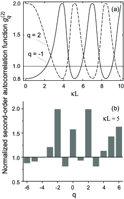
Figure 4: Normalized second-order autocorrelation function $g_{q}^{(2)}$ as a function of (a) the effective medium length $\kappa L$ and (b) the sideband order $q$ in the case of two-mode input. The input sideband $0$ is initially prepared in a Fock state, with $5$ photons. The input sideband $1$ is initially prepared in a thermal state, with 1 photon in average. In (a), the sideband order is $-1$ (solid line) and $2$ (dashed line). In (b), the effective medium length is $\kappa L=5$.

Unlike the case of single-mode input, in the case of two-mode input, the normalized second-order autocorrelation function $g_{q}^{(2)}=1+\Gamma_{q}^{(2)}/\langle\hat{n}_{q}\rangle^{2}$ depends, in general, on $\kappa L$ and $q$. Such behavior is illustrated in Fig. 4. When $\kappa L$ is such that $J_{q}(\kappa L)=0$ or $J_{q-\nu}(\kappa L)=0$, we have $g_{q}^{(2)}=g_{\nu}^{(2)}(0)$ or $g_{q}^{(2)}=g_{0}^{(2)}(0)$, respectively. Consequently, if the two input sidebands have different normalized autocorrelation functions, i.e., $g_{0}^{(2)}(0)\not=g_{\nu}^{(2)}(0)$, then, with increasing $\kappa L$ or $q$, the normalized autocorrelation function $g_{q}^{(2)}$ will oscillate between the values $g_{0}^{(2)}(0)$ and $g_{\nu}^{(2)}(0)$ [see Fig. 4]. In particular, if the photon statistics of one of the input fields, e.g., the sideband $0$, is sub-Poissonian [$g_{0}^{(2)}(0)<1$] and that of the other input field is super-Poissonian [$g_{\nu}^{(2)}(0)>1$], then each generated sideband $q$ will have complex statistical properties and will oscillate between sub-Poissonian [$g_{q}^{(2)}<1$] and super-Poissonian [$g_{q}^{(2)}>1$] photon statistics [see Fig. 4]. Using the prepared Raman coherence $\rho_{0}$ or the medium length $L$ as a control parameter, we can switch a sideband field from super-Poissonian photon statistics to sub-Poissonian or vice versa. Similar modulation of photon statistics has been demonstrated in a linear directional coupler coupler .

IV.2 Modulation of squeezing

We study the mixing and modulation of the squeezing properties of the sideband fields. When we use Eq. (4) to calculate the amplitudes $\langle\hat{b}_{q}\rangle$ and $\langle\hat{b}_{q}^{2}\rangle$ of the sidebands generated from the initial state (35), we find the expressions

$$\langle\hat{b}_{q}\rangle=e^{iq\pi/2}J_{q}(\kappa L)\langle\hat{b}_{0}(0)\rangle+e^{i(q-\nu)\pi/2}J_{q-\nu}(\kappa L)\langle\hat{b}_{\nu}(0)\rangle$$ (40)

and

$$\langle\hat{b}_{q}^{2}\rangle = e^{iq\pi}J_{q}^{2}(\kappa L)\langle\hat{b}_{0}^{2}(0)\rangle+e^{i(q-\nu)\pi}J_{q-\nu}^{2}(\kappa L)\langle\hat{b}_{\nu}^{2}(0)\rangle$$

$$\mbox{}+2e^{i(q-\nu/2)\pi}J_{q}(\kappa L)J_{q-\nu}(\kappa L)\langle\hat{b}_{0}(0)\rangle\langle\hat{b}_{\nu}(0)\rangle.$$

We insert Eqs. (36), (40), and (LABEL:21) into Eq. (19). Then, we obtain the squeezing factor

$$S_{q}(\varphi+q\pi/2) = J_{q}^{2}(\kappa L)S_{0}^{\mathrm{(in)}}(\varphi)$$ (42)

$$\mbox{}+J_{q-\nu}^{2}(\kappa L)S_{\nu}^{\mathrm{(in)}}(\varphi+\nu\pi/2),$$

where $S_{0}^{\mathrm{(in)}}$ and $S_{\nu}^{\mathrm{(in)}}$ are the initial squeezing factors of the sidebands $0$ and $\nu$, respectively. As seen, the squeezing factor $S_{q}$ of the sideband $q$ is a superposition of the input squeezing factors $S_{0}^{\mathrm{(in)}}$ and $S_{\nu}^{\mathrm{(in)}}$, taken with the quadrature phase shifts $-q\pi/2$ and $-(q-\nu)\pi/2$, respectively, and weighted by the factors $J_{q}^{2}(\kappa L)$ and $J_{q-\nu}^{2}(\kappa L)$, respectively.

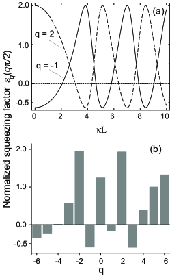
Figure 5: Normalized squeezing factor $s_{q}(q\pi/2)$ as a function of (a) the effective medium length $\kappa L$ and (b) the sideband order $q$ in the case of two-mode input. The input sideband $0$ is initially prepared in a squeezed vacuum state, with the squeezing parameter $r=1$ and the phase $\theta=0$. The input sideband $1$ is initially prepared in a thermal state, with the mean photon number 1. In (a), the sideband order is $-1$ (solid line) and $2$ (dashed line). In (b), the effective medium length is $\kappa L=5$.

Unlike the case of single-mode input, in the case of two-mode input, the normalized squeezing factor $s_{q}(\varphi+q\pi/2)=S_{q}(\varphi+q\pi/2)/\langle\hat{n}_{q}\rangle$ varies, in general, with $\kappa L$ and $q$. Such behavior is illustrated in Fig. 5. When $\kappa L$ is such that $J_{q}(\kappa L)=0$ or $J_{q-\nu}(\kappa L)=0$, we have $s_{q}(\varphi+q\pi/2)=s_{\nu}^{\mathrm{(in)}}(\varphi+\nu\pi/2)$ or $s_{q}(\varphi+q\pi/2)=s_{0}^{\mathrm{(in)}}(\varphi)$, respectively. Consequently, if the normalized squeezing factors $s_{0}^{\mathrm{(in)}}(\varphi)$ and $s_{\nu}^{\mathrm{(in)}}(\varphi+\nu\pi/2)$ of the two input fields are different, the normalized squeezing factor $s_{q}(\varphi+q\pi/2)$ will oscillate between the values $s_{0}^{\mathrm{(in)}}(\varphi)$ and $s_{\nu}^{\mathrm{(in)}}(\varphi+\nu\pi/2)$. In particular, if one of the two input fields, e.g., the sideband $0$, is squeezed [$s_{0}^{\mathrm{(in)}}(\varphi_{0})<0$] and the other input field is not squeezed [$s_{\nu}^{\mathrm{(in)}}(\varphi)>0$], then, each generated sideband $q$ will have complex squeezing properties and will oscillate between a squeezed state [$s_{q}(\varphi_{0}+q\pi/2)<0$] and a non-squeezed state [$s_{q}(\varphi)>0$], see Fig. 5. Using the prepared Raman coherence $\rho_{0}$ or the medium length $L$ as a control parameter, we can switch a sideband field from a non-squeezed state to a squeezed state or vice versa. Note that a similar result has been obtained for a linear directional coupler coupler .

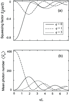
Figure 6: (a) Squeezing factor $S_{q}(q\pi/2)$ and (b) mean photon number $\langle\hat{n}_{q}\rangle$ as functions of the effective medium length $\kappa L$ in the case where the sideband $0$ is initially prepared in a weak squeezed vacuum state and the sideband $1$ is initially prepared in a strong coherent state. The parameters for the initial states of the input sidebands are $r=1$, $\theta=0$, and $\alpha=20$. The curves are calculated for the sidebands $0$ (solid line), $1$ (dashed line), and $3$ (dotted line).

We analyze a particular case where the sideband $0$ is initially in a squeezed vacuum state $|\xi\rangle_{0}=\exp[(\xi^{*}\hat{b}_{0}^{2}-\xi\hat{b}_{0}^{\dagger 2})/2]|0\rangle_{0}$ and the sideband $\nu$ is initially in a coherent state $|\alpha\rangle_{\nu}$. Here, $\xi=re^{i\theta}$ is a complex number, the modulus $r=|\xi|$ characterizes the amount of squeezing, and the phase angle $\theta$ characterizes the alignment of the squeezed vacuum state in phase space. For the input sideband $0$, we have Mandel and Scully book $\langle\hat{b}_{0}^{\dagger}(0)\hat{b}_{0}(0)\rangle=\sinh^{2}r$, $\langle\hat{b}_{0}(0)\rangle=0$, and $S_{0}^{\mathrm{(in)}}(\varphi)=\cosh 2r-\cos(2\varphi-\theta)\sinh 2r-1$. For the input sideband $\nu$, we have $\langle\hat{b}_{\nu}^{\dagger}(0)\hat{b}_{\nu}(0)\rangle=|\alpha|^{2}$, $\langle\hat{b}_{\nu}(0)\rangle=\alpha$, and $S_{\nu}^{\mathrm{(in)}}(\varphi)=0$. Then, we find from Eq. (36) that the mean photon number of an arbitrary sideband $q$ is

$$\langle\hat{b}_{q}^{\dagger}\hat{b}_{q}\rangle=J_{q}^{2}(\kappa L)\sinh^{2}r+J_{q-\nu}^{2}(\kappa L)|\alpha|^{2}.$$ (43)

We find from Eq. (42) that the maximal squeezing of the sideband $q$ occurs in the $\varphi_{q}$-quadrature where $\varphi_{q}=\theta/2+q\pi/2$. The corresponding value of the squeezing factor is

$$S_{q}(\varphi_{q})=J_{q}^{2}(\kappa L)(e^{-2r}-1).$$ (44)

As seen from Eq. (44), squeezing can be transferred from the initial squeezed vacuum state of the sideband $0$ to the other sidebands. The squeezing factors of the sidebands are independent of the amplitude $\alpha$ of the initial coherent state of the sideband $\nu$. Meanwhile, the mean photon number of each sideband is governed not only by the squeezing parameter $r$ of the initial state of the sideband $0$ but also by the amplitude $\alpha$ of the initial state of the sideband $\nu$. Using this fact, we can manipulate to get optimized mean photon numbers and squeezing degrees of the sideband fields at the output as per requirement. In particular, we can convert squeezing from a weak field to a much stronger field. To illustrate this possibility, we plot in Fig. 6 the squeezing factor $S_{q}(q\pi/2)$ and the mean photon number $\langle\hat{n}_{q}\rangle$ as functions of the effective medium length $\kappa L$ for the parameters $r=1$, $\theta=0$, $\nu=1$, and $\alpha=20$. In this case, the most negative value of the input squeezing factor $S_{0}^{\mathrm{(in)}}(\varphi)$ is achieved at $\varphi=0$ and is given by $S_{0}^{\mathrm{(in)}}(0)=e^{-2r}-1\cong-0.86$, indicating the squeezing degree 86%. The mean photon number of the input squeezed vacuum state is $\langle\hat{b}_{0}^{\dagger}(0)\hat{b}_{0}(0)\rangle=\sinh^{2}r\cong 1.38$, rather small. The solid lines in Fig. 6 show that the sideband $0$, initially prepared in a weak squeezed vacuum state, can be significantly enhanced while keeping its squeezing degree substantial. Meanwhile, the dashed lines show that, for $\kappa L=1.84$, the sideband $1$, initially prepared in a strong coherent state, is squeezed by about 29% and has the mean photon number of about 41. Similarly, the dotted lines show that, for $\kappa L=4.2$, a generated new sideband $3$ is squeezed by about 16% and has the mean photon number of about 39. Thus, from a weak squeezed field at the input, we can obtain other output squeezed fields that have smaller but still substantial squeezing degrees, much larger mean photon numbers, and different frequencies.

IV.3 Two-photon interference

We show the possibility of quantum interference between the probability amplitudes for a pair of photons with different frequencies in the coherent Raman process. We assume that the sidebands $0$ and $1$ are initially prepared in independent single-photon states. This initial condition corresponds to the situation where two photons with different frequencies $\omega_{0}$ and $\omega_{1}$ are incident into the Raman medium. The input state of the fields can be written as

$$|\Psi_{\mathrm{in}}\rangle=|1\rangle_{0}|1\rangle_{1}\prod_{q\not=0,1}|0\rangle_{q}=\hat{b}_{0}^{\dagger}(0)\hat{b}_{1}^{\dagger}(0)|0\rangle.$$ (45)

The output state of the fields is given by $|\Psi_{\mathrm{out}}\rangle=\hat{b}_{0}^{\dagger}(-L/c)\hat{b}_{1}^{\dagger}(-L/c)|0\rangle$. With the help of Eq. (4), we find

$$|\Psi_{\mathrm{out}}\rangle = -i\sqrt{2}\sum_{q}e^{iq\pi}J_{q}(\kappa L)J_{q-1}(\kappa L)|2_{q}\rangle$$ (46)

$$\mbox{}-i\sum_{k<l}e^{i(k+l)\pi/2}[J_{k}(\kappa L)J_{l-1}(\kappa L)$$

$$\mbox{}+J_{l}(\kappa L)J_{k-1}(\kappa L)]|1_{k}1_{l}\rangle.$$

Here, the Fock state $|2_{q}\rangle$ is the state of two photons in the sideband $q$ with no photons in the other sidebands, and the Fock state $|1_{k}1_{l}\rangle$ is the state in which there is one photon in each of the sidebands $k$ and $l$ but no photons in the other sidebands.

It follows from Eq. (46) that the probability for finding two photons in the sideband $q$ is

$$W_{q}^{(2)}=2J_{q}^{2}(\kappa L)J_{q-1}^{2}(\kappa L).$$ (47)

The joint probability for finding one photon in each of the sidebands $k$ and $l$ ($k\not=l$) is given by

$$W_{kl}=[J_{k}(\kappa L)J_{l-1}(\kappa L)+J_{l}(\kappa L)J_{k-1}(\kappa L)]^{2}.$$ (48)

The probability $W_{q}^{(1)}=\sum_{l\not=q}W_{ql}$ for having one and only one photon in the sideband $q$ is

$$W_{q}^{(1)}=J_{q}^{2}(\kappa L)+J_{q-1}^{2}(\kappa L)-4J_{q}^{2}(\kappa L)J_{q-1}^{2}(\kappa L).$$ (49)

The mean photon number of the sideband $q$ is

$$\langle\hat{n}_{q}\rangle=J_{q}^{2}(\kappa L)+J_{q-1}^{2}(\kappa L).$$ (50)

We find the relations $W_{-q}^{(2)}=W_{1+q}^{(2)}$, $W_{-q}^{(1)}=W_{1+q}^{(1)}$, and $\langle\hat{n}_{-q}\rangle=\langle\hat{n}_{1+q}\rangle$, which reflect the symmetry of the generated Stokes and anti-Stokes sidebands with respect to the two input sidebands 0 and 1.

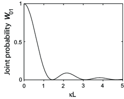
Figure 7: Joint probability $W_{01}$ for finding one photon in each of the sidebands $0$ and $1$ as a function of the effective medium length $\kappa L$.

When we insert $k=0$ and $l=1$ into Eq. (48), we obtain the following expression for the joint probability for finding one photon in each of the sidebands $0$ and $1$:

$$W_{01} = [J_{0}^{2}(\kappa L)-J_{1}^{2}(\kappa L)]^{2}.$$ (51)

This expression shows that the joint probability $W_{01}$ may become zero at certain values of $\kappa L$ [see Fig. 7]. This is a signature of destructive interference between two channels that form the state $|1_{0}1_{1}\rangle$. In the first channel, each of the two photons individually transmits through the medium without any changes. The two-photon probability amplitude for this channel is $J_{0}(\kappa L)J_{0}(\kappa L)=J_{0}^{2}(\kappa L)$. In the second channel, both the photons are scattered from the prepared Raman coherence and exchange their sidebands. The two-photon probability amplitude for this channel is $e^{i\pi/2}J_{1}(\kappa L)e^{i\pi/2}J_{1}(\kappa L)=-J_{1}^{2}(\kappa L)$. Since Raman scattering produces a phase shift of $\pi/2$ for each photon, the probability amplitudes for the two channels (the transmission and scattering of both the photons) are $180^{\circ}$ out of phase. The interference between the two channels is therefore destructive, yielding the output state $|1_{0}1_{1}\rangle$ with the joint probability $W_{01}$ given above. When the medium length $L$ is such that $J_{0}^{2}(\kappa L)=J_{1}^{2}(\kappa L)$, the interference between the two two-photon amplitudes becomes completely destructive, and therefore the state $|1_{0}1_{1}\rangle$ is removed from the output state (46). We denote such a medium length by $L_{f}$. The positions of the zeros of $W_{01}$ depicted in Fig. 7 indicate that the first three values of $L_{f}$ are given by $\kappa L_{f}=1.44$, 3.11, and 4.68. It is interesting to note that $\kappa L_{f}$ can be determined in an experiment using a single-mode input. Indeed, in the case where a single sideband $0$ is initially excited, the mean photon numbers of the generated sidebands are given by Eq. (8). Therefore, the effective medium length $\kappa L_{f}$ corresponds to the situation where the probe sideband $0$ and its adjacent sidebands $\pm 1$ have the same mean photon numbers at the output.

There exist literatures on two-photon interference in various systems Hong ; applications ; Qbeat . Two-photon interference in coherent Raman scattering, described above, is an analogy of two-photon interference at a conventional beam splitter Hong ; Mandel and Scully book . We emphasize that two-photon interference in coherent Raman scattering involves copropagating photons with different frequencies in a collinear scheme.

IV.4 General relation between the $P$ representations of the input and output states

To be more general, we consider the case where an arbitrary number of sidebands is initially excited. We find that an arbitrary multimode coherent state $|\{\alpha_{q}(0)\}\rangle$ of the input fields produces a coherent state $|\{\alpha_{q}(L/c)\}\rangle$ of the output fields. Here, the output amplitudes $\{\alpha_{q}(L/c)\}$ are linearly transformed from the input amplitudes $\{\alpha_{q}(0)\}$ as given by

$$\alpha_{q}(L/c)=\sum_{q^{\prime}}e^{i(q-q^{\prime})\pi/2}J_{q-q^{\prime}}(\kappa L)\alpha_{q^{\prime}}(0).$$ (52)

Consequently, the diagonal coherent-state representation $P_{\mathrm{in}}(\{\alpha_{q}\})$ of an arbitrary input quantum state $\hat{\rho}_{\mathrm{in}}$ determines the representation $P_{\mathrm{out}}(\{\alpha_{q}\})$ of the output state $\hat{\rho}_{\mathrm{out}}$ via the equation

$$P_{\mathrm{out}}(\{\alpha_{q}\})=P_{\mathrm{in}}(\{\alpha^{\prime}_{q}\}).$$ (53)

Here, we have introduced the notation

$$\alpha^{\prime}_{q}=\sum_{q^{\prime}}e^{-i(q-q^{\prime})\pi/2}J_{q-q^{\prime}}(\kappa L)\alpha_{q^{\prime}}.$$ (54)

If the input state $\hat{\rho}_{\mathrm{in}}$ is a classical state Mandel and Scully book , $P_{\mathrm{in}}(\{\alpha_{q}\})$ must be non-negative and less singular than a $\delta$ function, and consequently so must $P_{\mathrm{out}}(\{\alpha_{q}\})$. In this case, the output state $\hat{\rho}_{\mathrm{out}}$ is also a classical state. Moreover, since the multimode coherent state $|\{\alpha_{q}\}\rangle$ is separable and the weight factor $P_{\mathrm{out}}(\{\alpha_{q}\})$ is non-negative, the output state $\hat{\rho}_{\mathrm{out}}$ is, by definition, separable Chuang ; Zeilinger . Therefore, a necessary condition for the output fields to be in an inseparable (entangled) state or, more generally, in a nonclassical state is that the input field state is a nonclassical state. A similar condition has been derived for the beam splitter entangler Knight . Note that, in the case where we use a single-mode input field $q=0$, prepared in an arbitrary quantum state with the coherent-state representation $P_{\mathrm{in}}^{(0)}(\alpha)$ (the Stokes and anti-Stokes sideband fields are initially in the vacuum state), Eq. (53) becomes

$$P_{\mathrm{out}}(\{\alpha_{q}\})=P_{\mathrm{in}}^{(0)}(\alpha^{\prime}_{0})\prod_{q\not=0}\delta(\alpha^{\prime}_{q}).$$ (55)

It has been shown in Ref. entang that, when the input field is prepared in an even or odd coherent state, a multipartite entangled coherent state can be generated.

V Conclusions and discussions

We have studied the quantum properties of multiorder sidebands generated by the beating of a quantum probe field with a prepared Raman coherence in a far-off-resonance medium. Under the conditions of negligible dispersion and limited bandwidth, we have derived a Bessel-function solution for the sideband field operators. We have analytically and numerically calculated various quantum statistical characteristics of the multiorder sideband fields.

We have examined the quantum properties of the sideband fields in the case of single-mode quantum input. We have shown that, when we change the effective medium length or the Raman sideband order, the autocorrelation functions, the cross-correlation functions, the photon-number distributions, and the squeezing factors undergo oscillations governed by the Bessel functions. When the sideband order is higher, the onset of the sideband generation occurs later and, therefore, so does the onset of the sideband autocorrelation functions. The mean photon number and the autocorrelation functions of each sideband reach their largest values at the same optimal medium length determined by the first peak of the corresponding Bessel function. The higher the sideband order, the larger is the optimal length and the smaller is the maximal output values of the mean photon number and sideband autocorrelation functions.

Meanwhile, the normalized autocorrelation functions and normalized squeezing factors of the probe field are not altered by the parametric beating process. They are replicated into the comb of generated multiorder sidebands. As the result, the single-mode input field and the generated sidebands have identical normalized autocorrelation functions and identical normalized squeezing factors. In other words, they have similar quantum statistical properties – the same type of photon statistics and the same type of squeezing. In addition to this resemblance, it has been shown that an input field in a coherent state can produce sideband fields in coherent states. It has also been shown that, when the input field is prepared in a thermal state, the reduced state of each generated sideband is also a thermal state. Therefore, the multiorder coherent Raman process can be used to multiplex the statistical properties of a quantum probe field into a broad comb of different frequencies.

As far as replicating the statistical properties of the input probe into its sidebands is concerned, the Raman medium appears to behave as a linear system. However, the replication of the normalized autocorrelation functions and normalized squeezing factors of the probe field does not mean the replication of the quantum state at all. The photon-number distributions and the quantum states of the sidebands evolve in a rather complicated way. Cross-correlations between the sidebands can be generated from initially uncorrelated fields. An inseparable state can be generated from a separable nonclassical state. Although the dynamics of our model system is linear with respect to the field variables, the possibilities of interesting quantum phenomena such as anti-correlation generation, squeezing multiplexing, and entangled-state generation represent the quantum properties that cannot be described by the classical statistics of the fields with positive $P$ functions.

We have also studied the mixing and modulation of photon statistical properties in the case of two-mode quantum input. We have shown that the prepared Raman coherence and the medium length can be used as control parameters to switch a sideband field from one type of photon statistics to another type, or from a non-squeezed state to a squeezed state and vice versa. In addition, we can switch nonclassical properties, such as sub-Poissonian photon statistics and squeezing, from one frequency to another frequency. We have also shown an example of quantum interference between the probability amplitudes for a pair of photons with different frequencies.

We have made interesting observations that the multiorder coherent Raman scattering behaves in many aspects as a conventional beam splitter and hence can be called a multiorder Raman beam splitter. The two systems have the same underlying physics: the fields are linearly transformed from the input values. However, the two systems are different in their natures. Unlike the conventional beam splitter, the multiorder coherent Raman process can efficiently produce a broad comb of sideband fields whose frequencies are different and are separated by integer multiples of the Raman modulation frequency. The number of generated Raman sidebands increases with the effective medium length, which is proportional to the product of the medium length and the prepared Raman coherence. The Bessel functions of the effective medium length play a similar role as the transmission and reflection coefficients of a conventional beam splitter.

The ability of the far-off-resonance Raman medium to generate a broad comb of fields with similar quantum statistical properties and to switch the quantum statistical characteristics of the radiation fields from one type to another type may find useful applications for high-performance optical communication networks. In addition, two-photon interference in coherent Raman scattering may find various applications for high-precision measurements and also for quantum computation.

Finally, we emphasize that the coupling between the Raman sidebands can be controlled by the magnitude of the prepared Raman coherence, that is, by the intensities of the driving fields. In a realistic far-off-resonance Raman medium, such as molecular hydrogen or deuterium vapor Modulation ; D2 , solid hydrogen subfem ; Kien99 , and rare-earth doped dielectrics kolesov , a large Raman coherence and, consequently, a large number of Raman sidebands can be generated by the two-color adiabatic pumping technique. In such a system, the generation of a broad comb of high-order Raman sidebands with nonclassical statistical properties is, in principle, feasible. Therefore, we expect that the coherent Raman scattering technique using quantum fields will become a practical and efficient method for a wide range of applications in nonlinear and quantum optics.

References

- (1) V. P. Kalosha and J. Herrmann, Phys. Rev. Lett. 85, 1226 (2000); V. P. Kalosha and J. Herrmann, Opt. Lett. 26, 456 (2001); Fam Le Kien, Nguyen Hong Shon, and K. Hakuta, Phys. Rev. A 64, 051803(R) (2001); Fam Le Kien, K. Hakuta, and A. V. Sokolov, ibid. 66, 023813 (2002); V. Kalosha, M. Spanner, J. Herrmann, and M. Ivanov, Phys. Rev. Lett. 88, 103901 (2002); R. A. Bartels, T. C. Weinacht, N. Wagner, M. Baertschy, Chris H. Greene, M. M. Murnane, and H. C. Kapteyn, ibid. 88, 013903 (2002).
- (2) J. Q. Liang, M. Katsuragawa, Fam Le Kien, and K. Hakuta, Phys. Rev. Lett. 85, 2474 (2000).
- (3) M. Katsuragawa, J. Q. Liang, Fam Le Kien, and K. Hakuta, Phys. Rev. A 65, 025801 (2002).
- (4) A. Nazarkin, G. Korn, M. Wittmann, and T. Elsaesser, Phys. Rev. Lett. 83, 2560 (1999).
- (5) S. E. Harris and A. V. Sokolov, Phys. Rev. A 55, R4019 (1997); A. V. Sokolov, D. D. Yavuz, and S. E. Harris, Opt. Lett. 24, 557 (1999); A. V. Sokolov, D. D. Yavuz, D. R. Walker, G. Y. Yin, and S. E. Harris, Phys. Rev. A 63, 051801(R) (2001).
- (6) A. V. Sokolov, D. R. Walker, D. D. Yavuz, G. Y. Yin, and S. E. Harris, Phys. Rev. Lett. 85, 562 (2000).
- (7) S. E. Harris and A. V. Sokolov, Phys. Rev. Lett. 81, 2894 (1998).
- (8) Fam Le Kien, J. Q. Liang, M. Katsuragawa, K. Ohtsuki, K. Hakuta, and A. V. Sokolov, Phys. Rev. A 60, 1562 (1999).
- (9) Fam Le Kien and K. Hakuta, Phys. Rev. A 67, 033808 (2003).
- (10) R. Kolesov and O. Kocharovskaya, Phys. Rev. A 67, 023810 (2003).
- (11) A. V. Sokolov, D. R. Walker, D. D. Yavuz, G. Y. Yin, and S. E. Harris, Phys. Rev. Lett. 87, 033402 (2001).
- (12) N. Zhavoronkov and G. Korn, Phys. Rev. Lett. 88, 203901 (2002).
- (13) S. E. Harris, D. R. Walker, and D. D. Yavuz, Phys. Rev. A 65, 021801(R) (2002).
- (14) H. P. Yuen and J. H. Shapiro, IEEE Trans. Inf. Theory IT-26, 78 (1980); M. Ley and R. Loudon, Opt. Commun. 54, 317 (1985); B. Yurke, S. L. McCall, and J. R. Klauder, Phys. Rev. A 33, 4033 (1986); S. Prasad, M. O. Scully, and W. Martienssen, Opt. Commun. 62, 139 (1987); Z. Y. Ou, C. K. Hong, and L. Mandel, Opt. Commun. 63, 118 (1987); H. Fearn and R. Loudon, Opt. Commun. 64, 485 (1987); R. A. Campos, B. E. A. Saleh, and M. C. Teich, Phys. Rev. A 40, 1371 (1989).
- (15) C. K. Hong, Z. Y. Ou, and L. Mandel, Phys. Rev. Lett. 59, 2044 (1987).
- (16) J. Torgerson, D. Branning, C. Monken, and L. Mandel, Phys. Lett. A 204, 323 (1995); K. Mattle, H. Weinfurter, P. G. Kwiat, and A. Zeilinger, Phys. Rev. Lett. 76, 4656 (1996); D. Bouwmeester, J. Pan, K. Mattle, M. Eibl, H. Weinfurter, and A. Zeilinger, Nature (London) 390, 575 (1997); T. C. Ralph, N. K. Langford, T. B. Bell, and A. G. White, Phys. Rev. A 65, 062324 (2002); T. B. Pittman, B. C. Jacobs, and J. D. Franson, Phys. Rev. Lett. 88, 257902 (2002); S. P. Walborn, A. N. de Oliveira, S. Padua, and C. H. Monken, Phys. Rev. Lett. 90, 143601 (2003).
- (17) M. S. Kim, W. Son, V. Bužek, and P. L. Knight, Phys. Rev. A 65, 032323 (2002); Wang Xiang-bin, ibid. 66, 024303 (2002).
- (18) W. K. Lai, V. Bužek, and P. L. Knight, Phys. Rev. A 43, 6323 (1991); Janszky, C. Sibilia, and M. Bertolotti, J. Mod. Opt. 35, 1757 (1988).
- (19) L. Mandel and E. Wolf, Optical Coherence and Quantum Optics (Cambridge University Press, New York, 1995); M. Scully and S. Zubairy, Quantum Optics (Cambridge University Press, New York, 1997).
- (20) L. J. Wang, C. K. Hong, and S. R. Friberg, J. Opt. B: Quantum Semiclass. Opt. 3, 346 (2001).
- (21) M. D. Lukin, A. B. Matsko, M. Fleischhauer, and M. O. Scully, Phys. Rev. Lett. 82, 1847 (1999); A. S. Zibrov, A. B. Matsko, O. Kocharovskaya, Y. V. Rostovtsev, G. R. Welch, and M. O. Scully, ibid. 88, 103601 (2002).
- (22) Fam Le Kien, A. K. Patnaik, and K. Hakuta (submitted to Phys. Rev. A).
- (23) Z. Y. Ou and L. Mandel, Phys. Rev. Lett. 61, 54 (1988); Z. Y. Ou and L. Mandel, ibid. 62, 2941 (1989); H. Huang and J. H. Eberly, J. Mod. Optics 40, 915 (1993); M. O. Scully, U. W. Rathe, C. Su, and G. S. Agarwal, Opt. Commun. 136, 39 (1997); A. K. Patnaik and G. S. Agarwal, J. Mod. Optics 45, 2131 (1998).
- (24) The Physics of Quantum Information, edited by D. Bouwmeester, A. K. Ekert, and A. Zeilinger (Springer, New York, 2000).
- (25) M. A. Nielsen and I. L. Chuang, Quantum Computation and Quantum Information (Cambridge University Press, New York, 2000).