Relaxation and dephasing in a many-fermion generalization of the Caldeira-Leggett model

Abstract

We analyze a model system of fermions in a harmonic oscillator potential under the influence of a fluctuating force generated by a bath of harmonic oscillators. This represents an extension of the well-known Caldeira-Leggett model to the case of many fermions. Using the method of bosonization, we calculate Green’s functions and discuss relaxation and dephasing of a single extra particle added above the Fermi sea. We also extend our analysis to a more generic coupling between system and bath, that results in complete thermalization of the system.

The interaction between a system and its environment is an important fundamental issue in quantum mechanics. It is at the basis of relaxation phenomena (like spontaneous emission), is essential for the measurement process, and leads to the destruction of interference effects (“decoherence” or “dephasing”). In the theory of quantum-dissipative systemsweiss , there are only few exactly solvable models, most notably the Caldeira-Leggett modelcallegg of a single particle coupled to a bath of harmonic oscillators. This is the simplest possible model in which friction and fluctuations appear. If the particle is free, then this model can be used to study the quantum analogue of Brownian motion. The model remains exactly solvable if the particle moves in a parabolic potential (the damped quantum harmonic oscillator).

However, in many solid state applications, we actually consider dephasing of an electron inside a Fermi sea. It is difficult to apply the insights gained from single-particle calculations in such cases, since the Pauli principle may play an important role in relaxation processes. There have been comparatively few detailed studies of quantum-dissipative many-particle systems. Among them we mention a general discussion of dephasing in a Luttinger liquid OpenLuttLiquids , a study of fermions coupled to independent baths indepFermions , and a formally exact extension of the Feynman-Vernon influence functional to fermions FV-Fermi . In other cases, the Pauli principle has been introduced “by hand”, by keeping only the thermal part of the bath spectrum key-9 .

In this Letter, we study a natural extension of the Caldeira-Leggett model to a many-fermion case. The model consists of a sea of fermions populating the lower energy levels of a harmonic oscillator. We are interested in the effects that arise when a bath is coupled to this system via a fluctuating spatially homogeneous force. In contrast to an analogous system of free fermions ABring , the bath leads to transitions between levels, with strong effects of the Pauli principle. This model might also prove relevant to the discussion of cold fermionic atoms in a $1d$ harmonic trap key-12 ; wonneberger under the influence of fluctuations of the trapping potential.

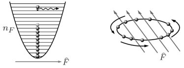
Figure 1: Left: Fermions in an oscillator, coupled to a dissipative bath via a fluctuating force $\hat{F}$. Right: Approximately equivalent model of chiral fermions on a ring, subject to a transverse force.

We rewrite and solve the Hamiltonian using the method of bosonization, for the case of large particle numbers. This enables us to evaluate Green’s functions and to describe relaxation and dephasing of an extra particle added above the Fermi sea. Finally, we will extend our model to a more generic type of coupling.

The model - We consider a system of $N$ identical fermions (non-interacting and spinless) confined in a one-dimensional harmonic oscillator potential (see Fig. 1). A fluctuating force $\hat{F}$ leads to a coupling of the form $\hat{F}\sum_{j}\hat{x}_{j}$, yielding, in second quantization:

$$\hat{H}=\omega_{0}\sum_{n=0}^{\infty}n\hat{c}_{n}^{\dagger}\hat{c}_{n}+\hat{H}_{B}+$$

$$\frac{\hat{F}}{\sqrt{2m\omega_{0}}}\sum_{n=0}^{\infty}\sqrt{n+1}(\hat{c}_{n+1}^{\dagger}\hat{c}_{n}+h.c.)$$ (1)

The operators $\hat{c}_{n}$ annihilate fermions in the oscillator levels $n$. The bath Hamiltonian $\hat{H}_{B}$ describes an infinite number of harmonic oscillators, and the force $\hat{F}$ is a sum over the bath normal coordinates $\hat{Q}_{j}$. It is characterized fully by its power spectrum $\left\langle\hat{F}\hat{F}\right\rangle_{\omega}$. The special case of an Ohmic bath, used for Quantum Brownian motion callegg , has $\left\langle\hat{F}\hat{F}\right\rangle_{\omega}=(\eta\omega/\pi)\theta(\omega_{c}-\omega)\theta(\omega)$ at $T=0$, where $\eta=m\gamma$ is the friction coefficient, $\gamma$ the damping rate, and $\omega_{c}$ the cutoff. As the form of the coupling (1) is not translationally invariant, the frequency $\omega_{0}$ contains a stabilizing countertermcallegg ; weiss ; inpreparation .

Effectively, the force acts only on the center-of-mass (c.m.) motion of the particles which, for the harmonic oscillator, is independent of the relative motion. Thus, in principle our model reduces to a single damped harmonic oscillator, analyzed in Ref. callegg . However, we are interested in single-fermion properties, and not in the collective c.m. motion itself. Although the problem can be solved exactly via normal modes of the complete set of oscillators and antisymmetrizing with respect to fermion coordinates, this procedure gets extremely cumbersome. Instead, we employ an approximation for large fermion numbers $N$, which also allows an extension to a more generic coupling between system and bath.

Bosonization - For sufficiently large $N$ the lowest levels are always occupied (at the given interaction strength and temperatures), i.e. excitations are confined to the region near the Fermi level. Then we may employ the method of bosonization, rewriting the energy of fermions as a sum over boson modes wonneberger . This is possible since the energies of the oscillator levels increase linearly with quantum number, just as the kinetic energy in the Luttinger model of interacting electrons in one dimension (for recent reviews see DelftSchoeller ).

We introduce (approximate) boson operators $\hat{b}_{q}=\frac{1}{\sqrt{q}}\sum_{n=0}^{\infty}\hat{c}_{n}^{\dagger}\hat{c}_{n+q}$ ($q\geq 1$), which destroy particle-hole excitations. Then, the Hamiltonian given above becomes approximately

$$\hat{H}\approx\omega_{0}\sum_{q=1}^{\infty}q\hat{b}_{q}^{\dagger}\hat{b}_{q}+\sqrt{\frac{N}{2m\omega_{0}}}\hat{F}(\hat{b}_{1}+\hat{b}_{1}^{\dagger})+\hat{H}_{B}+E_{\hat{N}}\,,$$ (2)

which will form the basis of our analysis. Here $E_{\hat{N}}=\omega_{0}\hat{N}(\hat{N}-1)/2$ is the total energy of the $N$-fermion noninteracting ground state. Eq. (2) reveals that $\hat{F}$ only couples to the lowest boson mode ($q=1$), corresponding to the c.m. motion. The damped motion of the c.m. oscillator can be solved exactly, along the lines of Ref. callegg or key-10 , providing us with correlators such as $\left\langle\hat{b}_{1}(t)\hat{b}_{1}^{\dagger}(0)\right\rangle$.

Derivation of Green’s functions - In order to find the Green’s functions, we have to go back from the boson operators $\hat{b}_{q}$ to the fermion operators $\hat{c}_{n}$, by employing well-known finite-size bosonization identities. In our case, we first have to introduce auxiliary fermion operators $\hat{\psi}(x)$:

$$\hat{\psi}(x)=\frac{1}{\sqrt{2\pi}}\sum_{n}e^{inx}\hat{c}_{n},\,\hat{c}_{n}=\frac{1}{\sqrt{2\pi}}\int_{0}^{2\pi}e^{-inx}\hat{\psi}(x)\,dx$$ (3)

The coordinate $x$ does not refer to the motion in the oscillator. Rather, we have effectively mapped our problem to a chiral Luttinger liquid on a ring with a coupling $\propto\hat{F}\cos(x)$ ($x\in[0,2\pi[$), see Fig. 1 (right). Thus, the following results also describe relaxation of momentum states in that model. Although a generic discussion of dissipative Luttinger liquids has been provided in OpenLuttLiquids , the particular questions we are going to study have not been analyzed before.

The operators $\hat{\psi}(x)$ may be expressed asDelftSchoeller :

$$\hat{\psi}(x)=\hat{K}\hat{\lambda}(x)e^{i\hat{\varphi}^{\dagger}(x)}e^{i\hat{\varphi}(x)}=\hat{K}\hat{\lambda}e^{i\hat{\phi}}r\,,$$ (4)

with

$$\hat{\phi}=\hat{\varphi}+\hat{\varphi}^{\dagger},\,\,\hat{\varphi}(x)=-i\sum_{q=1}^{\infty}\frac{1}{\sqrt{q}}e^{iqx}\hat{b}_{q}\,.$$ (5)

The “Klein factor” $\hat{K}$ annihilates a particle, with $[\hat{K},\hat{b}_{q}^{(\dagger)}]=0$ and $\hat{K}(t)=\hat{K}\exp(-i\omega_{0}(\hat{N}-1)t)$. We have $\hat{\lambda}(x)=\exp(i(\hat{N}-1)x)/\sqrt{2\pi}$ and $r\equiv\exp(-[\hat{\varphi}^{\dagger},\hat{\varphi}]/2)$. (The exponent in $r$ diverges, so a formal cutoff at high $q$ should be introduced, which will drop out in the end result)

Using Eq. (3), we find for the hole-propagator:

$$\left\langle\hat{c}_{n^{\prime}}^{\dagger}(t)\hat{c}_{n}\right\rangle=\frac{1}{2\pi}\int_{0}^{2\pi}e^{i(n^{\prime}x^{\prime}-nx)}\left\langle\hat{\psi}^{\dagger}(x^{\prime},t)\hat{\psi}(x,0)\right\rangle\,dx\,dx^{\prime}\,.$$ (6)

The $\hat{\psi}$-Green’s function is given directly in terms of the $\hat{\phi}$-correlator, using Eq. (4):

$$\left\langle\hat{\psi}^{\dagger}(x^{\prime},t)\hat{\psi}(x,0)\right\rangle=\frac{r^{2}}{2\pi}e^{in_{F}((x-x^{\prime})+\omega_{0}t)}\left\langle e^{-i\hat{\phi}(x^{\prime},t)}e^{i\hat{\phi}(x,0)}\right\rangle$$ (7)

(with $n_{F}=N-1$). The expectation value on the right-hand side may be evaluated exactly DelftSchoeller , since the system-bath coupling is bilinear. This yields $\exp(E)$ with:

$$E=-\frac{1}{2}\left(\left\langle\hat{\phi}(x^{\prime},t)^{2}\right\rangle+\left\langle\hat{\phi}(x,0)^{2}\right\rangle\right)+\left\langle\hat{\phi}(x^{\prime},t)\hat{\phi}(x,0)\right\rangle$$ (8)

The correlator of $\hat{\phi}$ is a polynomial in $X\equiv\exp(ix)$ and $X^{\prime}\equiv\exp(ix^{\prime})$ (see Eq. (5)). Now the double Fourier integral in Eq. (6) may be evaluated by expanding $\exp(E)$ as a series in $X$ and $X^{\prime}$. We find that $\left\langle\hat{c}_{n^{\prime}}^{\dagger}(t)\hat{c}_{n}\right\rangle$ is the coefficient of $X^{n}/X^{\prime n^{\prime}}$ in the expansion of

$$e^{\delta E(X,X^{\prime},t)}\sum_{k\leq n_{F}}e^{i\omega_{0}kt}(X/X^{\prime})^{k}\,,$$ (9)

where the noninteracting exponent has been subtracted in $\delta E=E-E_{(0)}$, which thus contains only the correlator of the damped c.m. mode $q=1$. Detailed plots of the Green’s function will be published elsewhere inpreparation . Here we provide the result in the weak-coupling approximation, where we neglect the bath-induced smearing of the equilibrium Fermi level and use an exponential decay for the c.m. motion. Both assumptions are summarized in $\left\langle\hat{b}_{1}(t)\hat{b}_{1}\right\rangle=\left\langle\hat{b}_{1}^{\dagger}(t)\hat{b}_{1}\right\rangle=0$ and $\left\langle\hat{b}_{1}(t)\hat{b}_{1}^{\dagger}(0)\right\rangle=e^{-i\omega^{\prime}_{0}t-\Gamma t/2}$ ($\omega^{\prime}_{0}$ is the renormalized c.m. frequency, and $\Gamma$ is the decay rate, with $\Gamma=N\gamma$ for the Ohmic bath). Then, the exact Eq. (9) yields

$$\left\langle\hat{c}_{n}^{\dagger}(t)\hat{c}_{n}\right\rangle\approx e^{i\omega_{0}nt}\sum_{m=0}^{n_{F}-n}\frac{\nu(t)^{m}}{m!}\,,$$ (10)

where $\nu(t)\equiv\exp(-i(\omega_{0}^{{}^{\prime}}-\omega_{0})t-\Gamma t/2)-1$.

We find that the hole (particle) propagator does not decay to zero in the limit $t\rightarrow\infty$, for any $n<n_{F}-1$ ($n>n_{F}+2$), since $\nu(t)\rightarrow-1$. This is in contrast to the naive single-particle picture of complete decay for any level $n\neq n_{F},n_{F}+1$ not directly at the Fermi level (i.e. the result suggested by the leading order self-energy). Physically, adding a hole (particle) creates an excited many-particle state which also contains contributions where the c.m. mode is not excited, and these will not decay, because only the c.m. mode is damped. A more generic coupling, leading to ergodicity, will be discussed at the end of this Letter.

Time-evolution of density matrix - We now turn to the two-particle Green’s function in order to learn about relaxation of level populations and dephasing. Consider placing an electron in a superposition of levels above the Fermi sea, creating the many-particle state $\sum_{n_{0}}\Psi_{n_{0}}\hat{c}_{n_{0}}^{\dagger}\left|FS\right\rangle$ at time $0$. We assume the levels $n_{0}$ to be unoccupied. This will hold for $n_{0}>n_{F}$ in the weak-coupling limit, for which the following results have been evaluated. The reduced single-particle density matrix evolves according to:

$$\rho_{nn^{\prime}}(t)=\sum_{n_{0},n_{0}^{\prime}}\Psi_{n_{0}}\Psi_{n_{0}^{\prime}}^{*}\left\langle\hat{c}_{n_{0}^{\prime}}\hat{c}_{n^{\prime}}^{\dagger}(t)\hat{c}_{n}(t)\hat{c}_{n_{0}}^{\dagger}\right\rangle\,.$$ (11)

We may rewrite the Green’s function in Eq. (11) in terms of $\hat{\psi}(x)$ (Eq. (3)), leading to a four-fold Fourier integral, analogous to Eq. (6). Using Eq. (4), this may be evaluated by a series expansion in four exponentials $\exp(ix^{(^{\prime})})$, $\exp(iy^{(^{\prime})})$, similar to Eq. (9). We omit the lengthy general formula inpreparation , but discuss a limiting case below.

In Fig. 2, we have plotted the resulting time-evolution of the density matrix for the case of an equal superposition of two levels, $\Psi_{n_{1}}=\Psi_{n_{2}}=1/\sqrt{2}$, at $T=0$.

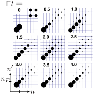
Figure 2: Time-evolution of the single-particle density matrix $\rho_{nn^{\prime}}(t)$ (Eq. (11)), after placing an extra particle in a superposition of two states. The radius of each circle gives $\left|\rho_{nn^{\prime}}(t)\right|$. Levels $n,n^{\prime}=n_{F}-1,\ldots,n_{F}+6$ are indicated by grid lines. For this example $\omega_{0}-\omega_{0}^{\prime}=2\Gamma$.

The population of the highest occupied states in the Fermi sea (lower left of panels) decreases, because these fermions become partly excited at the expense of the extra particle, due to the effective interaction mediated by the bath. Moreover, the particle does not decay all the way down to the lowest unoccupied state $n_{F}+1$. Rather, in the long-time limit, the excitation is distributed over a range of levels above the Fermi level, up to the initial levels $n_{1,2}$. Again, this is because only the c.m. mode couples to the bath, such that a fraction of the initial excitation energy remains in the system. The same is true of the coherences, i.e. the off-diagonal elements in the density matrix.

High initial excitation - These generic features can be analyzed in more detail for the case of a high initial excitation energy ($n_{0}-n_{F}\gg 1$). Then, the expression for $\rho$ can be given explicitly in a relatively simple form:

$$\rho_{nn^{\prime}}(t)=\sum_{n_{0},n_{0}^{\prime}}\Psi_{n_{0}}\Psi_{n_{0}^{\prime}}^{*}e^{i\omega_{0}(n_{0}^{\prime}-n_{0})t}\delta_{n_{0}-n,n_{0}^{\prime}-n^{\prime}}\times$$

$$[\rho_{{\rm decay}}(n_{0}-n,t)+\rho_{{\rm heat}}(n-n_{F}-1,n^{\prime}-n_{F}-1,t)]$$ (12)

The decay of the excitation is described by

$$\rho_{{\rm decay}}(m,t)=\frac{(-1)^{m}}{m!}\left(\nu(t)+\nu^{*}(t)\right)^{m}e^{\nu(t)+\nu^{*}(t)}\,,$$ (13)

where $m=n_{0}-n=n_{0}^{\prime}-n^{\prime}$ may be interpreted as the net number of quanta transferred to the bath (Fig. 3, left). At short times, $\Gamma t\ll 1$, the nonvanishing entries are $\rho_{{\rm decay}}(1,t)\approx\Gamma t$ and $\rho_{{\rm decay}}(0,t)\approx 1-\Gamma t$, i.e. Golden Rule behaviour is recovered (both for relaxation, $n_{0}=n_{0}^{\prime}$, and dephasing, $n_{0}\neq n_{0}^{\prime}$). In the long-time limit we get a stationary distribution, $\rho_{{\rm decay}}(m,t)\rightarrow(2^{m}/m!)e^{-2}$.

“Heating” around the Fermi level is encoded in (see Fig. 3)

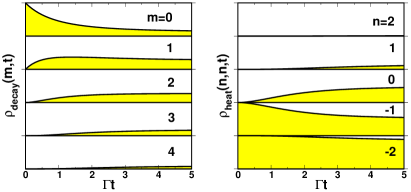
Figure 3: Generic time evolution of density matrix in the limit of high initial excitation (Eqs. (12)-(14); plot for $\omega_{0}^{\prime}=\omega_{0}$).

$$\rho_{{\rm heat}}(n,n^{\prime},t)=\nu(t)^{n-n^{\prime}}\sum\frac{\left|\nu(t)\right|^{2(\tilde{m}_{1}+\tilde{m}_{2})}}{m_{1}!m_{2}!\tilde{m}_{1}!\tilde{m}_{2}!}(-1)^{m_{2}+\tilde{m}_{2}}\,,$$ (14)

where the triple sum runs over $\tilde{m}_{1}={\rm max}(0,n^{\prime}+1)\ldots\infty,$ $\tilde{m}_{2}=0\ldots\infty$, $m_{1}={\rm max}(0,\tilde{m}_{2}+n+1)\ldots n-n^{\prime}+\tilde{m}_{1}+\tilde{m}_{2}$, and we have $m_{2}=\tilde{m}_{1}+\tilde{m}_{2}-m_{1}+n-n^{\prime}$. In the short-time limit, $\rho_{{\rm heat}}(n,n,t)$ approximates to $1$ for $n<-1$, to $1-|\nu(t)|^{2}$ for $n=-1$, to $|\nu(t)|^{2}$ for $n=0$, and $0$ for $n>0$ (to $O(|\nu|^{2})$), describing the unperturbed Fermi sea and the onset of heating. Comparing to the full results (Fig. 2), we find that the limiting case (12) is a very good approximation even for small excitation energies.

Generic coupling - Up to now, we have considered a coupling where the particle coordinates enter linearly, and consequently only the c.m. mode is damped.

We now extend our analysis to a more generic situation, replacing the interaction in Eq. (2) by:

$$\sqrt{\frac{N}{2m\omega_{0}}}\hat{F}\sum_{q=1}^{\infty}f_{q}\sqrt{q}(\hat{b}_{q}+\hat{b}_{q}^{\dagger})\,.$$ (15)

Now the bath induces transitions between levels $n+q$ and $n$, with an arbitrary (real-valued) amplitude $\propto f_{q}$ (which, however, must not depend on $n$). For $f_{1}=1,\,f_{q}=0\,(q>1)$ we recover the original model. For $f_{q}\neq 0$ all the boson modes are damped and couple to each other via the bath. Formally, the correlators $\left\langle\hat{b}_{q^{\prime}}(t)\hat{b}_{q}^{\dagger}\right\rangle$ can be written in terms of the resolvent of the classical problem of boson oscillators coupled to bath oscillators (inpreparation , compare key-10 ).

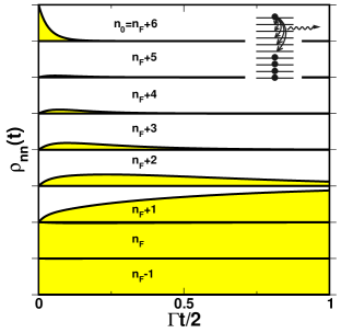
Figure 4: Decay of populations for a bath inducing transitions between levels that are arbitrarily far apart (see text).

The correlator $\left\langle\hat{\phi}(x^{\prime},t)\hat{\phi}(x,0)\right\rangle$ now contains contributions for all pairs $q,q^{\prime}$. The evaluation of the Green’s functions proceeds as before. Unfortunately, one has to deal with far more terms. However, interesting behaviour is already found in the weak-coupling limit, which here implies neglecting the effective coupling between boson modes that has been induced by the bath, and describing the correlator of each boson mode separately as a damped oscillation.

For the case of constant $f_{q}=1$ (up to some cutoff) and an Ohmic bath spectrum, the boson correlator decay rate ($\propto q\left\langle\hat{F}\hat{F}\right\rangle_{\omega=q\omega_{0}}$, see Eq. (15)) equals $q^{2}\Gamma/2$. This fits the expectation about Pauli blocking: The decay of a particle from state $n_{F}+\delta n+1$ is due to transitions by $1$ to $\delta n$ levels, and adding up their rates (which grow linearly) leads to a total rate $\propto\delta n^{2}$, consistent with the decay rate of the highest boson mode $q=\delta n$ that is excited by adding this particle. The actual evolution of the Green’s function is a superposition of decays, with rates up to this value.

An example for the resulting time-evolution is shown in Fig. 4: Starting from a state where a single extra particle has been added in level $n_{0}$ above the Fermi sea, one can observe the evolution of the populations $\rho_{nn}(t)$ (Ohmic bath, $T=0$). At intermediate times, heating around the Fermi level takes place (barely visible, in contrast to Fig. 2). In contrast to the previous case, the relaxation towards the $N+1$-particle ground state is complete, the system is ergodic.

Conclusions - We have analyzed a many-fermion generalization of the single particle in a damped harmonic oscillator, illustrating relaxation and dephasing in a dissipative many-particle system. Using the method of bosonization (in the limit of large particle number), we have derived exact expressions for the Green’s functions and discussed them in limiting cases. We have analyzed the decay of an excited state created by adding one particle above the Fermi level, where one can observe the “heating” around the Fermi level (due to the effective interaction between particles), as well as the incomplete decay of the excited particle. Finally, we have extended our analysis to a more generic type of coupling between system and bath, where the system becomes fully ergodic.

- (1) U. Weiss: Quantum Dissipative Systems, World Scientific, Singapore (2000).
- (2) A. O. Caldeira and A. J. Leggett, Physica 121A, 587 (1983); Phys. Rev. A 31, 1059 (1985).
- (3) A. H. C. Neto, C. D. Chamon, C. Nayak, Phys. Rev. Lett. 79, 4629 (1997).
- (4) J. M. Wheatley, Phys. Rev. Lett. 67, 1181 (1991). P. C. Howell and A. J. Schofield, cond-mat/0103191.
- (5) D. S. Golubev and A. D. Zaikin, Phys. Rev. B 59, 9195 (1999).
- (6) B. L. Altshuler, A. G. Aronov, and D. E. Khmelnitsky, J. Phys. C Solid State 15, 7367 (1982); S. Chakravarty and A. Schmid, Phys. Rep. 140, 195 (1986). A. Stern, Y. Aharonov, and Y. Imry, Phys. Rev. A 41, 3436 (1990); D. Cohen and Y. Imry, Phys. Rev. B 59, 11143 (1999).
- (7) F. Marquardt and C. Bruder, Phys. Rev. B 65, 125315 (2002).
- (8) F. Schreck et al., Phys. Rev. Lett. 87, 080403 (2001); S. R. Granade et al., ibid. 88, 120405 (2002); T. Loftus et al., ibid. 88, 173201 (2002); A. Recati et al., ibid. 90, 020401 (2003).
- (9) W. Wonneberger, Phys. Rev. A 63, 063607 (2001); G. Xianlong and W. Wonneberger, Phys. Rev. A 65, 033610 (2002); G. Xianlong, F. Gleisberg, F. Lochmann, and W. Wonneberger, Phys. Rev. A 67, 023610 (2003); G. Xianlong and W. Wonneberger, J. Phys. B 37, 2363 (2004).
- (10) F. Marquardt and D. S. Golubev, cond-mat/0409401.
- (11) J. v. Delft and H. Schoeller, Annalen der Physik, Vol. 4, 225 (1998). H. Grabert, in ”Exotic States in Quantum Nanostructures” ed. by S. Sarkar, Kluwer (2001).
- (12) V. Hakim and V. Ambegaokar, Phys. Rev. A 32, 423 (1985).