Covariant description of spin $1/2$ particles in self–action

Abstract

The bispinor wave function finds its fundamental application in the study of electrons, neutrinos and protons as particles bound by their own potentials. Classical electromagnetism and the Dirac electron theory appear to be natural extensions of the physics that rules the electron itself. However, the charge density and the negative energy eigenvalues are two concepts which cannot survive further scrutiny. The electron and the proton resemble minute planetary systems where the bispinor terms defining their physical properties revolve with definite angular momentum around the singular point of the particles’ potentials. The mass of the electron–neutrino in relation to the electron’s and the mass of the latter in relation to the proton’s are determined under particular assumptions. The most important feature of the new approach is the faithful representation of free particles at rest with respect to inertial systems of reference. This certainly enhances the foundation of physics; precisely in the realm of Quantum Mechanics, where the customary description of free electrons is a confusing consequence of the limited scope of the Schrödinger and Dirac equations.

I General considerations

The free particle solutions of the Schrödinger equation, plane waves extending throughout space, bear no direct relation with the concept of particle that most of us may have. It is only natural that this circumstance gave rise to philosophical currents and crosscurrents from which no real consensus was ever obtained: on examining the probabilistic interpretation of the wave function, Niels Bohr arrived at the conclusion that science not necessarily should be concerned on whether or not the dynamic variables of the electron coexist with definite values. In essence, he argued that physical reality cannot be dissociated from the process of measurement. Consequently free electrons, which by definition do not interact even with measuring devises, remain metaphysical until their state of isolation is disrupted by experiment. Moreover, the Heisenberg uncertainty relations have revealed an intrinsic limitation in the accuracy that can be attained when the position and the momentum of the electron are measured simultaneously. Hence the entire formalism of Quantum Mechanics is to be considered as the tool for deriving predictions of statistical nature [1]

However, contrary to the familiar answer of the Copenhagen school, perhaps in accordance with Einstein’s faith in an objective reality, physics is sustained on the principle of inertia, which does not allow room for indeterminacies of the kind. For instance, the parameter of relative velocity appearing in the Lorentz transformations implies the presence of a particle at rest with respect to one of the inertial systems, and in uniform motion with respect to the other. Why? Because the relative velocity between systems of coordinates is devoid of physical meaning until a real object (particle) appears in space. We may ask, what sense does it make to verify the Lorentz covariance of the Dirac equation when the equation itself cannot describe a particle in isolation in accordance with the principle that makes the Lorentz transformation meaningful: the Galileo–Newton principle of inertia in the first place.

As a matter of fact, Erwin Schrödinger solved the hydrogen atom thinking of a proton fixed at the origin of an inertial system implied by the potential $r^{-1}$ in the equation. If the electron and the proton revolve around the center of mass, it is irrelevant for the point in question: it only means that in quantum mechanics one assumes that the atom remains fixed with respect to an inertial system. It follows, therefore, that in the attempt to preserve its conceptual consistency, quantum mechanics had to invoke the process of measurement or to rely on some other interpretation. Physics evolved leaving behind important conceptual problems unsolved. And so, some twenty years after the advent of the Schrödinger equation this problem emerged with a different face. Physicists became fully aware that, in order to complete the theory of the free electron, self–action had to be reckoned with. Then QED offered an approach based on the idea that the point–electron emits and absorbs virtual and real photons along its path. This time, however, the divergent self–energy put a definite end to the hope of a consistent theory, not to mention that the QED approach itself was inconsistent with the principle of inertia from the very outset, since the free electron path cannot be made to vanish with the choice of system of reference [2] .

Free electrons exist independently of experiment; we think that it is of the concern of physics to explain their existence in a way consistent with general principles. Fortunately, the framework to analyze the problem is defined already: the description of a self-interacting electron at rest with respect to an inertial system of reference should be carried out with the solutions of the one and only fundamental equation that can be proposed for the study of spin $1/2$ particles in self-action:

$$\gamma_{\mu}\left[{\partial_{\mu}+S_{\mu}(e,\nu,p)}\right]\,\psi\ =\ 0,$$ (1)

where $S_{\mu}$ represents the self–action 4–vector of the particle under study.

The conceptual structures of equation (1) and of the Dirac equation [3] ,

$$\gamma_{\mu}\,\left[\partial_{\mu}+\alpha\,A_{\mu}\right]\,\psi\ =\ -\,i\,\left(m\,c\,\hbar^{-1}\right)\,\gamma_{{}_{5}}\,\psi,$$ (2)

may reinforce each other in their own range of applicability and may fuse at some point too. The free particle solutions of the customary wave equations are important, but only as part in the solution of problems with discontinuous external interaction, either in space or in time. The tunnel effect –through the potential barriers that limit the force free region of the potential well– is a typical case where plane waves satisfying boundary conditions become necessary and meaningful also. Although, we suspect that plane waves with no boundary conditions are meaningless solutions which have misled physicists for over 75 years now.

II The electron self–potentials

Mostly every physicist knows that the energy of a point electron diverges; although not every physicist is well aware that Gauss’ law cannot hold when the particle is deprived of physical dimensions. Indeed, the volume integral of the last two expressions below reveals a contradiction:

$$\nabla\cdot\vec{\textrm{E}}\ =\ r^{-2}\partial_{r}(r^{2}\,\hat{\textrm{r}}\cdot\vec{\textrm{E}})\ =\ r^{-2}\partial_{r}(1)\ =\ 4\,\pi\,\delta(r).$$ (3)

The reason some textbooks invoke the divergence theorem to prove (3) correct is easy to understand: empty space cannot be the origin of the Coulomb potential. Interesting enough, this is not the only case where physical problems have been circumvented at the expense of mathematical congruence. Paul Dirac himself had the opinion that renormalization has defied all the attempts of the mathematician to make it sound [4] ; yet, such procedures have advocates and detractors who may never convince one another.

It is appropriate to recall that the functional dependence of the potential on the charge density brings about problems of its own. For example, who can tell if the electrostatic energy of an electron is localized where the potential and the charge density coexist or is it dispersed throughout space?

$${\cal E}\ =\ \int\limits_{\textrm{\tiny{electron}}}{\rho\,\phi}\ =\ \int\limits_{\textrm{\tiny{all space}}}{\nabla\phi\cdot\nabla\phi}.$$ (4)

More important, the association of the square of the electrostatic field with the energy density leads to the following conclusion: the ratio of electromagnetic momentum over electromagnetic energy of an electron in uniform motion is incompatible with relativity [5] .

Experience shows that each and every electron in a given distribution contributes with their individual Coulomb potential to the total potential. However, if the electron happens to be a particle with physical dimension, there is no reason to think that a small portion of its volume would contribute with a small portion to its Coulomb potential. Again, since there is no consistent model of the electron, the physics that make its existence possible is not known.

The vanishing of the Laplacian of the inverse distance occurs in three dimensions only:

$$\nabla^{2}_{\textrm{N}}\left(\sum_{k\,=\,1}^{\textrm{N}}{x_{k}^{2}}\right)^{-1/2}\ =\ 0\qquad\Rightarrow\qquad\textrm{N}\ =\ 3.$$ (5)

In fact, this is a mathematical characteristic of the Coulomb potential inherent to the electron. This is a postulate and it is incompatible with the concept of charge density.

The task now is to adjust the electromagnetic theory to a new conceptual structure. We shall do that in parts and as the circumstance allows. It is convenient to say in advance that suitable combinations of the products of the four components of the wave function and their complex conjugates enable the construction of covariant densities. These densities play an essential role in the definitions of the electromagnetic inertia and of the other properties of the electron; all of which properties will vanish beyond a small radius from the singular point of the potential (from now on “singularity” for short). In this way the Coulomb potential springs up from the inside of the electron; though, no functional relation with any of the covariant densities exists.

Electromagnetic signals from the singularity necessarily relate to the 4-vector of null length, $r_{\alpha}=(\vec{\textrm{r}},r)$. The contraction of $r_{\alpha}$ with the 4-velocity of the singular point,

$$u_{\alpha}\ =\ (\vec{\textrm{u}},1)\,(1-\textrm{u}^{2})^{-1/2}\ \to\,(\vec{\textrm{0}},1),$$ (6)

yields the fundamental invariant involved in the Lienard-Wiechert potentials

$$\textrm{I}_{0} =\ -(r_{\alpha}\,u_{\alpha})^{-1}\,\to\,r^{-1},$$ (7)

$$A_{\alpha} =\ \textrm{I}_{0}\,u_{\alpha}\ =\ (\vec{\textrm{u}},1)\,(r-\vec{\textrm{r}}\cdot\vec{\textrm{u}})^{-1}\ \to\ (\vec{\textrm{0}},r^{-1}),$$

(the arrow reads –for a particle at rest reduces to–).

Direct consequence of their genesis, these potentials satisfy the fundamental differential equations

$$\partial_{\alpha}\,\partial_{\alpha}\,A_{\beta}\ =\ 0,$$ (9)

$$\partial_{\alpha}\,A_{\alpha}\ =\ 0,$$ (10)

Consequently, the field tensor $F_{\alpha\beta}=\partial_{\alpha}\,A_{\beta}-\partial_{\beta}\,A_{\alpha}$ satisfies Maxwell’s equations with no sources:

$$\partial_{\alpha}\,F_{\beta\gamma}+\partial_{\gamma}\,F_{\alpha\beta}+\partial_{\beta}\,F_{\gamma\alpha}\ =\ 0,$$ (11)

$$\partial_{\alpha}\,F_{\alpha\beta}\ =\ 0,$$ (12)

In order to write in a concise manner the potentials of a continuous distribution of electrons in arbitrary motion, one may assume that the customary equations, $\partial_{\alpha}\,\partial_{\alpha}\,A_{\beta}=-J_{\beta}$ and $\partial_{\alpha}\,A_{\alpha}=0$, hold. However, in this case $J_{\beta}$ would represent the piecewise differentiable functions best approximating the 4-current of singularities. The vanishing of the 4–divergence  $\partial_{\alpha}\,J_{\alpha}$   states the conservation of the net number of singular points.

The repulsive Coulomb potential alone is not sufficient to get square integrable solutions. Tentatively, the second potential that is necessary for this purpose could be thought of as the quantum version of the vector potential of a point magnet: $(\lambda_{e}/2)\,(\vec{\sigma}\times\vec{\textrm{r}}\,\,r^{-3})$, where $\vec{\sigma}$ represents the $4\times 4$ Pauli spin matrices, and   $\lambda_{e}$   is a length–parameter measuring the strength of the coupling, not to be fixed before hand. The reader may wish to verify that the substitution of the matrix potential in equation (1) is entirely equivalent to the substitution of the imaginary vector $-\,i\,\lambda_{e}r^{-2}\,\hat{r}$. The covariant form of this 3–vector enters as part of the self–action 4–vector:

$$S_{\mu}(e)=-\alpha\,A_{\mu}+i\,\lambda_{e}\sigma_{\mu}=-\alpha\,\textrm{I}_{0}\,u_{\mu}+i\,\lambda_{e}\partial_{\mu}\,\textrm{I}_{0}$$

$$\to\qquad-\alpha\,(\vec{\textrm{0}},r^{-1})-i\,\lambda_{e}(r^{-2}\hat{r},0)$$ (13)

The electromagnetic coupling constant in the equation above means that the electron was assumed to repel itself with the same strength that two electrons repel each other. Now, the imaginary radial potential is also indispensable for the description of the electron–neutrino. As neutrinos may not have magnetic moment, perhaps this gauge invariant ($\sigma_{\alpha\beta}=\partial_{\alpha}\sigma_{\beta}-\partial_{\beta}\sigma_{\alpha}=0$) new entity in physics is not related to magnetic moment but to the spin. For simplicity, the coupling constant $\lambda_{e}$ was considered to be the same for both particles. Eventually we will relate $\alpha$ to $\lambda_{e}$, which in turn could relate $\alpha$ to $m_{\nu}/m_{e}$ if $\lambda_{e}$ is written in terms of $m_{e},\,m_{\nu},\,\hbar$ and $c$. There are two options:

$$\lambda_{e}\ =\ \frac{\beta\,\hbar}{m_{e}\,c},$$ (14)

where $\beta=m_{\nu}/m_{e}$. Interchanging the mass parameters would be the second option, but it does not work.

III The electron solutions

An electron in self–action is a state with definite energy which is taken into account with the factor $\exp(-i\,E\,t/\hbar)$ in the solutions. Since the potentials are radial, the spatial part of the two independent solutions is to be written as shown [3] .

First solution:

$$\psi_{1} =\left[\frac{j+1-m}{2(j+1)}\right]^{1/2}F\,Y_{j+\frac{1}{2},m-\frac{1}{2}}\to\frac{F\,Y_{1,0}}{\sqrt{3}}$$ (15)

$$\psi_{2} =-\left[\frac{j+1+m}{2(j+1)}\right]^{1/2}F\,Y_{j+\frac{1}{2},m+\frac{1}{2}}\to\sqrt{\frac{2}{3}}\,F\,Y_{1,1}$$

$$\psi_{3} =i\left[\frac{j+m}{2j}\right]^{1/2}G\,Y_{j-\frac{1}{2},m-\frac{1}{2}}\to i\,G\,Y_{0,0}$$

$$\psi_{4} =i\left[\frac{j-m}{2j}\right]^{1/2}G\,Y_{j-\frac{1}{2},m+\frac{1}{2}}\to 0.$$

Second solution:

$$\psi_{1} =i\left[\frac{j+m}{2j}\right]^{1/2}L\,Y_{j-\frac{1}{2},m-\frac{1}{2}}\to i\,L\,Y_{0,0}$$ (16)

$$\psi_{2} =i\left[\frac{j-m}{2j}\right]^{1/2}L\,Y_{j-\frac{1}{2},m+\frac{1}{2}}\to 0$$

$$\psi_{3} =\left[\frac{j+1-m}{2(j+1)}\right]^{1/2}K\,Y_{j+\frac{1}{2},m-\frac{1}{2}}\to\frac{K\,Y_{1,0}}{\sqrt{3}}$$

$$\psi_{4} =-\left[\frac{j+1+m}{2(j+1)}\right]^{1/2}K\,Y_{j+\frac{1}{2},m+\frac{1}{2}}\to\sqrt{\frac{2}{3}}\,K\,Y_{1,1}.$$

The spherical harmonics are already normalized to one. The arrow indicates that the one and only value of the total angular momentum in conceptual connection with the problem is $j=1/2$. ($m=1/2$ is our option). The substitution of the sum of these solutions in equation (1) yields two identical systems of differential equations, each containing only one pair of radial functions, $(F,G)$ or $(K,L)$. We may leave functions $(K,L)$ aside for a while and work with functions $(F,G)$:

$$\partial_{r}F+\frac{2F}{r}-\frac{\lambda_{e}\,F}{r^{2}}\ = \left[\frac{E}{\hbar c}-\frac{\alpha}{r}\right]\,G$$ (17a)

$$\partial_{r}G-\frac{\lambda_{e}\,G}{r^{2}}\ = -\left[\frac{E}{\hbar c}-\frac{\alpha}{r}\right]\,F$$ (17b)

The substitutions

$$r =\frac{e^{2}}{E}\,s,\quad\alpha=\frac{e^{2}}{\hbar c},\quad\beta=\frac{m_{\nu}}{m_{e}},\quad\gamma=\frac{E}{mc^{2}},$$

$$F =F\,^{\dagger}\,\exp(-\alpha^{-1}\beta\,\gamma\,s^{-1}),$$

$$G =G\,^{\dagger}\,\exp(-\alpha^{-1}\beta\,\gamma\,s^{-1}),$$

reduce the system to

$$s^{-2}\partial_{s}(s^{2}\,F\,^{\dagger})=(1-s^{-1})\,\alpha\,G\,^{\dagger}$$ (18a)

$$\partial_{s}\,G\,^{\dagger}=-(1-s^{-1})\,\alpha\,F\,^{\dagger}$$ (18b)

The reader may verify that the two independent solutions,$(F,G)$ and $(f,g)$, can be written as:

$$\sum_{k\,=\,0}^{\infty}{G_{k}^{\dagger}(\alpha,s)}=a_{0}+\sum_{k\,=\,1}^{\infty}{G_{k}^{\ddagger}(s)\,\alpha^{2k}},$$

$$\sum_{k\,=\,0}^{\infty}{F_{k}^{\dagger}(\alpha,s)}=\sum_{k\,=\,0}^{\infty}{F_{k}^{\ddagger}(s)\,\alpha^{2k+1}}$$ (19)

$$\sum_{k\,=\,0}^{\infty}{f_{k}^{\dagger}(\alpha,s)}=b_{0}\,s^{-2}+\sum_{k\,=\,1}^{\infty}{f_{k}^{\ddagger}(s)\,\alpha^{2k}},$$

$$\sum_{k\,=\,0}^{\infty}{g_{k}^{\dagger}(\alpha,s)}=\sum_{k\,=\,0}^{\infty}{g_{k}^{\ddagger}(s)\,\alpha^{2k+1}}$$ (20)

Concerning the first solution, function $G_{0}^{\dagger}$ is the constant $a_{0}$, and all the other functions as well as their first derivatives vanish at $s=1$. Concerning the second solution, function $f_{0}^{\dagger}=b_{0}\,s^{-2}$, and all the other functions, as in the former case, vanish in a smooth manner at the classical electron radius. The procedure for the obtainment of solutions in powers of $\alpha^{2}$ is iterative in nature and runs as follows.

In the first solution, the first step is to insert $G_{0}^{\dagger}$ into (18a). Integration is the second step. The constant of integration serves to force the vanishing of $f_{0}^{\dagger}$ at $s=1$:

$$s^{-2}\partial_{s}(s^{2}F_{0}^{\dagger})=(1-s^{-1})\,\alpha\,a_{0}$$

$$\Rightarrow\qquad F_{0}^{\dagger}=\alpha(a_{0}/6)(s^{-2}-3+2s).$$

We proceed with the insertion of $F_{0}^{\dagger}$ into (18b). Integration follows. The constant of integration forces the vanishing of $G_{1}^{\dagger}$ at $s=1$:

$$\partial_{s}\,G_{1}^{\dagger}=-(1-s^{-1})\,\alpha\,F_{0}^{\dagger}\qquad\Rightarrow$$

$$G_{1}^{\dagger}=-\alpha^{2}(a_{0}/12)[s^{-2}-2s^{-1}+6\ln\,s+9-10s+2s^{2}]$$

and so on. Notice that function $G^{\dagger}$ cuts the $s$–axis only once at $s^{2}\approx\alpha^{2}/12$.

In the second solution, the iterative procedure starts with the substitution of $f_{0}^{\dagger}=b_{0}\,s^{-2}$ into (18b), which yields function $g_{0}^{\dagger}$:

$$\partial_{s}\,g_{0}^{\dagger}=-(1-s^{-1})\,\alpha\,b_{0}\,s^{-2}$$

$$\Rightarrow\quad g_{0}^{\dagger}=-\alpha\,(b_{0}/2)\,(1-s)^{2}s^{-2}.$$

The reader may follow the prescription to get functions $f_{1}^{\dagger}$ and $g_{1}^{\dagger}$. With these functions at hand we may write down function $g^{\dagger}\,G^{\dagger}\,s^{-1}$ which will be useful hereinafter:

$$(g^{\dagger}\,G^{\dagger}\,s^{-1})\,s^{2}=\alpha\,\xi_{0}+\alpha^{3}\,\xi_{1}+...+\alpha^{2k+1}\,\xi_{k}+...$$ (21)

$$\xi_{0} =a_{0}\,b_{0}\,[s^{-1}-2+s],$$

$$\xi_{1} =-a_{0}\,b_{0}\,[s^{-3}-4s^{-2}+40-5s-36s^{2}$$

$$+4s^{3}+60s\ln\,s]/12$$

Since functions: $F,\,g,\,gG$ and $fF$ vanish in a smooth manner at $s=1$, the physical properties of the electron should be represented with covariant densities made up of the product of the two independent solutions: take for example the 4–vector

$$2\langle\psi_{a}\gamma_{\mu}\psi_{b}\rangle=(\psi_{a}+\psi_{b})\gamma_{\mu}(\psi_{a}+\psi_{b})^{*}$$

$$-\psi_{a}\gamma_{\mu}\psi_{a}^{*}-\psi_{b}\gamma_{\mu}\psi_{b}^{*}$$ (22)

where $\psi_{a}$ and $\psi_{b}$ are the two independent solutions. The time component of this 4–vector,

$$\langle\psi_{a}\gamma_{t}\psi_{b}\rangle=\frac{1}{3}|Y_{1,0}|^{2}\,Ff+\frac{2}{3}|Y_{1,1}|^{2}\,Ff+Y_{0,0}^{2}\,Gg$$ (23)

vanishes in a smooth manner at $s=1$ ($\gamma_{t}$ is the unit matrix). However, we cannot consider the solution $\psi=0$ for the region beyond $s=1$; because doing so would make functions $G$ and $f$ look like strings with a loose end (see figure 1).

Graphical discontinuities in the wave functions are not acceptable. This problem is solved by replacing the potential $\alpha\,A_{\mu}$ in favor of $(m_{e}\,c\,\hbar^{-1})\,u_{\mu}$ for the region beyond the classical electron radius. The corresponding radial equations are

$$\partial_{r}\,F+\frac{2\,F}{r}-\frac{\lambda_{e}\,F}{r^{2}} =\ \frac{E-m_{e}\,c^{2}}{\hbar\,c}\,G$$ (24a)

$$\partial_{r}\,G-\frac{\lambda_{e}\,G}{r^{2}} =\ -\frac{E-m_{e}\,c^{2}}{\hbar\,c}\,F$$ (24b)

Now we must set $E=m_{e}\,c^{2}$. With this consideration the external solutions,

$$G=a_{0}\,\exp(-\lambda_{e}\,r^{-1}),\qquad F=0,$$ (25)

$$f=b_{0}\,r^{-2}\,\exp(-\lambda_{e}\,r^{-1}),\qquad g=0,$$ (26)

join with the internal solutions (19) and (20) at the classical electron radius in a smooth manner. The external solutions have no further meaning since the corresponding bilinear products are null.

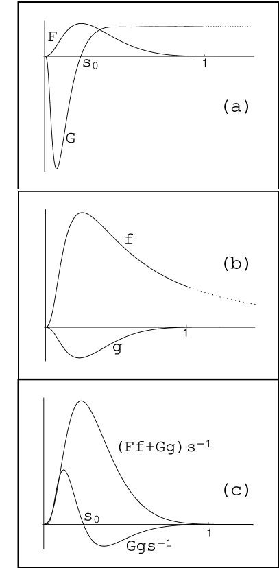
Figure 1: The graphs of the functions merely show their main features: all graphs vanish in a smooth manner at the origin of coordinates. (a) In the first independent solution, function $F$ is (roughly speaking) $\alpha$ times function $G$. Function $G$ cuts the $s$–axis only once at $s^{2}\approx\alpha^{2}/12$. Function $F$ vanishes in a smooth manner at $s=1$. Beyond $s=1$, function $G$ is essentially constant. (b) In the second independent solution, function $g$ is about $\alpha$ times function $f$; the former smoothly vanishes at $s=1$. Beyond this radius, $f$ decays essentially as $s^{-2}$. (c) The products of the functions vanish in a smooth manner at $s=1$. Beyond the classical electron radius the bilinear products are null. Thus, the energy of the electron is confined within its classical radius.

The bilinear function (22) could be named interaction–density, the recipient of the action of the Coulomb potential. Accordingly,

$${\cal E}\ =\ 4\,\pi\,m_{e}\,c^{2}\,\int_{0}^{1}{A_{\mu}(s)\,\langle\psi_{a}\,\gamma_{\mu}\,\psi_{b}\rangle}\,s^{2}\,ds$$ (27)

would represent the electromagnetic inertia of the electron. This definition, reminiscent of Maxwell’s expression (see equation (4)) is the formal substitution of the charge–density in favor of the interaction density. In Maxwell’s theory the charge density determines the electrostatic potential, whereas in the fundamental theory here being proposed the interaction density is determined by two potentials endowed with independent existence.

IV Further results

The incorporation of the Dirac fifth matrix ($\gamma_{5}$ in equation (2)) into this approach enables one to write down the whole set of covariant densities [3] .

The matrices,

$$\gamma_{t} =\ \textrm{diag}\,\left[1,1,1,1\right],$$

$$\gamma_{5} =\ \textrm{diag}\,\left[1,1,-1,-1\right],$$

$$\gamma_{x}\,\gamma_{y} =\ \textrm{diag}\,\left[i,-i,i,-i\right],$$

$$\gamma_{x}\,\gamma_{y}\,\gamma_{5} =\ \textrm{diag}\,\left[i,-i,-i,i\right].$$

and the table below are particularly important in this regard.

$$\begin{array}[]{ccc}\textrm{Pseudo Invariant}&\qquad 1&\qquad\textrm{none}\\ \textrm{Invariant}&\qquad 1&\qquad\left\langle{\psi_{a}\gamma_{5}\psi_{b}}\right\rangle\\ \textrm{4--vector}&\qquad 4&\qquad\left\langle{\psi_{a}\gamma_{t}\psi_{b}}\right\rangle\\ \textrm{pseudo 4--vector}&\qquad 4&\qquad\left\langle{\psi_{a}\gamma_{x}\gamma_{y}\psi_{b}}\right\rangle\\ \textrm{anti--symmetric tensor}&\qquad 6&\qquad\left\langle{\psi_{a}\gamma_{x}\gamma_{y}\gamma_{5}\psi_{b}}\right\rangle\end{array}$$

The first column shows the whole set of covariant densities. The second column indicates the number of components of each density. The third column shows the only component of the density that survives volume integration; the other components contain products of different spherical harmonics and their volume integral vanishes.

The transformation properties of $S_{z}=\langle\psi_{a}\gamma_{x}\gamma_{y}\psi_{b}\rangle$ and $M_{z}=\langle\psi_{a}\gamma_{x}\gamma_{y}\gamma_{5}\psi_{b}\rangle$, suggest to interpret the former as the z-component of spin-density and the latter as the $z$–component of magnetic polarization. From the matrices above and equations (15) and (16) we can see that $S_{z}$ is the same for the two independent solutions, $(F;G,f,g)$ and $(K,L,k,l)$. Though, $M_{z}$, corresponding to the first solution is opposite to $M_{z}$ of the second solution. Since electrons and positrons with the same spin orientation have opposite magnetic moments and the energy of both solutions is positive, perhaps the negative energy solutions of the Dirac equation, as well as the philosophy built up around them, need to be re–examined. Curiously enough, this is not the only case where physicists have thought that space itself has strange properties: Special Relativity came to show the futility of the study of the hydrodynamic properties the ether that presumably pervaded the whole universe.

The graph of the density of the electromagnetic inertia (see panel (c) of figure 1) invites the volume integral of the function $gGs^{-1}$ to vanish. This condition would interrelate $\alpha$ and $\beta$ and the electron would look as a minute planetary system wherein two electro-quarks (named so because of the appearance of fractions $1/3$ and $2/3$ in (23)) retain all the electromagnetic inertia while revolving around the singularity of the potentials. The covariant way of expressing this condition involves the Dirac fifth matrix $\gamma_{5}$: the density $\textrm{I}_{1}=u_{\mu}\,\langle\psi_{a}\gamma_{\mu}\psi_{b}\rangle$ is an invariant and so is $\textrm{I}_{2}=\langle\psi_{a}\gamma_{5}\psi_{b}\rangle$. Therefore, the vanishing of the volume integral of   $\textrm{I}_{0}(\textrm{I}_{1}-\textrm{I}_{2})$ is the condition we are talking about.

For the purpose of evaluating this integral it is important to notice the following:

1. If $s\gg 2\alpha^{-1}\,\beta=\eta$, function $W=\exp(-\eta\,s^{-1})$ is close to $1$.

2. Function $W$ starts bending downward for values of $s$ comparable to $\eta$.

3. For $s\ll\eta$, function $W$ is essentially null.

If $\eta$ is sufficiently small we have:

$$\int_{0}^{1}{W\,(1+s+s^{-2}+s^{-3})\,ds}\,\approx\,1+\frac{1}{2}+\eta^{-1}+\eta^{-2}.$$

Now,

$$\partial_{\eta}\,\int_{0}^{1}{W\,s^{-1}\,ds}=-\eta^{-1}\,\exp(-\eta)\,\approx\,-\eta^{-1}+1-\eta/2+...$$

Therefore

$$\int_{0}^{1}{W\,s^{-1}\,ds}=-\ln\,\eta+\eta-\eta^{2}/2!\,+...+c_{0}$$ (28)

The constant of integration $c_{0}\approx-0.51$ can be evaluated by plotting the graph of   $W\,s^{-1}$ (for $\eta=1$) and comparing the area under the graph with its analytical value given by the right hand side of (28) (evaluated for $\eta=1$).

When $\eta$ is small enough, the dominant term of the integral of $W\,\xi_{1}$ (see equation (21)) is the first one. All these considerations imply that the vanishing of the volume integral of $G\,g\,s^{-1}$ is congruent with the following approximation

$$-\ln\,\eta-0.51-2+1/2\ =\ (\alpha^{2}/12)\,\eta^{-2}.$$ (29)

Considering that   $m_{e}=511000$ eV and that $\alpha=1/137$, we get that the mass of the e–neutrino is larger than $1.75$ eV but smaller than $1.78$ eV. Hitherto experimental physics has set an upper limit of $2.2$ eV for $m_{\nu}$ [6] .

V The electron–neutrino solution

Equation (1) provides an amazingly simple solution to the electron–neutrino if it is regarded as an electron deprived of Coulomb potential. In this case the self–action would take this form:

$$S_{\mu}(\nu)\ =\ -m_{\nu}\,c\,\hbar^{-1}\,u_{\mu}+i\,\lambda_{e}\,\partial_{\mu}\,\textrm{I}_{0}$$ (30)

We already know the corresponding radial equations, yet there is only one solution of interest:

$$F\ =\ s^{-2}\,\exp(-\beta^{2}\,s^{-1}),\qquad G\ =\ 0$$ (31)

The fact that it is not possible to cut off the solution at any particular radius suggests the Copenhagen interpretation of the square of the wave function: the probability of the electron–neutrino to interact with matter beyond one wave length from the singularity of its own potential is

$$\left(\int_{1}^{\infty}{u_{\mu}\,\psi\,\gamma_{\mu}\,\psi^{*}\,s^{2}\,ds}\right)\,\left(\int_{0}^{\infty}{u_{\mu}\,\psi\,\gamma_{\mu}\,\psi^{*}\,s^{2}\,ds}\right)^{-1}$$

$$=\ 1-\exp(-2\,\beta^{2})\ \approx\ 2\,(m_{\nu}/m_{e})^{2}\ <\ 10^{-10}$$

Neutrinos $\mu$ and $\tau$ could be described with other coupling constants, ($\lambda_{\mu}$ and $\lambda_{\tau}$).

VI The proton

The description of the proton can be carried out thinking of it as a positron endowed with a Yukawa neutral meson field. Consider the scalar equation

$$\partial_{\alpha}\,\partial_{\alpha}\,\zeta\ =\ (m_{\pi_{0}}\,c\,\hbar^{-1})^{2}\,\zeta,$$ (32)

its time independent solution

$$\zeta\ =\ r^{-1}\exp[-(m_{\pi_{0}}\,c\,\hbar^{-1})\,r]$$

was used by Yukawa in his meson theory of the nuclear force [5] . In general, the nuclear force is attractive beyond the proton radius and repulsive for shorter distances, which prevents the nucleus from collapsing. Accordingly, the simplest self–action that we can think of is

$$S_{\mu}(p)\ =\ -n\,\zeta\,u_{\mu}-\alpha\,A_{\mu}+i\,\lambda_{e}\,\sigma_{\mu},$$ (33)

where $n$ is a dimensionless coupling constant which must vanish when the meson mass vanishes. The spin potential is assumed to be the same for the electron, the neutrino and the proton, all the offspring of neutron decay.

The solution of equation (1) for this case can be obtained following procedures very similar to the one used for the electron case. Moreover, it is not necessary to use numerical analysis for the obtainment of a good approximation when $n$ is one of the two simplest fundamental expressions: $n=m_{\pi_{0}}/m_{p}\approx 1/7$,  or $n=m_{\pi_{0}}\,m_{p}/(m_{\pi_{0}}+m_{p})^{2}\approx 1/9$. Actually, the correct value of   $m_{e}/m_{p}$   is obtained with the vanishing of the volume integral of $G\,g\,(\alpha\,\textrm{I}_{0}+n\,\zeta)$ when $n\approx 1/11$. Therefore, it can be inferred that the proton self–energy was defined as

$${\cal E}\ =\ 4\pi\,m_{p}c^{2}\int_{0}^{s_{0}}{(\alpha\,A_{\mu}+n\,\zeta\,u_{\mu})\,\langle\psi_{a}\,\gamma_{\mu}\,\psi_{b}\rangle\,s^{2}\,ds}$$ (34)

where $s_{0}$ is the radius where the right hand side of the corresponding radial equation vanishes.

This model can be improved to get a better approximation of $m_{e}/m_{p}$. However, we see a drawback of a different kind: the prevailing consensus is that protons are made up of three spin $1/2$ subparticles. Perhaps an attempt to express the GUT’s model in a covariant way should be made. How? assigning to each quark an individual bispinor wave function, yet all of them interrelated in a system of differential equations similar to (1).

One more interesting aspect of scalar equations is that the substitutions  $\psi(\vec{\textrm{r}},t)=\psi(\vec{\textrm{r}})\,\exp[-i\,(m\,c^{2}+E)\,t\,\hbar^{-1}]$ and $A_{\beta}\,\partial_{\beta}=c^{-1}\,\phi\,\partial_{t}$ in

$$(\partial_{\beta}\,\partial_{\beta}-2\,i\,\alpha\,A_{\beta}\,\partial_{\beta})\,\psi\ =\ (m^{2}\,c^{2}\,\hbar^{-2})\,\psi$$ (35)

yield

$$-(\hbar^{2}/2m)\,\nabla^{2}\,\psi+e^{2}\,\phi\,[1+(E/mc^{2})]\,\psi$$

$$=\ E\,\psi\,[1+(E/2mc^{2})].$$ (36)

Neglecting $E/mc^{2}$, which in atomic physics is much smaller than self–energy, the familiar Schrödinger equation is obtained. However, the important point is that imaginary vector potentials are necessary to yield differential equations with real coefficients. This is a feature of relativistic wave equations with the time–dependent factor $\exp(-i\,t\,\hbar^{-1})$. In fact, we had this situation with equation (1) and the potential  $i\,\lambda_{e}\,\sigma_{\mu}$.

As a final remark, the time–dependent factor $\exp\,(-E\,t\,\hbar^{-1})$ in equation (1) is a logical step to start investigating spin $1/2$ unstable particles.

References

- (1) Holland, R. Peter, The Quantum Theory of Motion, Cambridge University Press, 1993. Chapter 1 is a clear and concise presentation of the interpretations of Quantum Mechanics.
- (2) Selected papers on QED, Edited by Schwinger, S. J., Dover, 1958. The preface is an accessible overview of Quantum Electrodynamics.
- (3) Hill E.L. Rev. Mod. Phys. 10, 2, pp. 87-118, (1938). Potentials are assigned dimensions of inverse length. This reference is a magnificent monograph about the Dirac electron theory which is sufficient to follow this work in detail. Differences in notation exist but are easily identified.
- (4) Readings of Scientific American: Mathematics In The Modern World, (1968), pag 244.
- (5) The Feynman Lectures on Physics, Vol.2, Chap. 28, (1962)
- (6) http:/cupp.oulu.fi/neutrino/