Numerical Analysis of Boosting Scheme for Scalable NMR Quantum Computation

Abstract

Among initialization schemes for ensemble quantum computation beginning at thermal equilibrium, the scheme proposed by Schulman and Vazirani [L. J. Schulman and U. V. Vazirani, in Proceedings of the 31st ACM Symposium on Theory of Computing (STOC’99) (ACM Press, New York, 1999), pp. 322-329] is known for the simple quantum circuit to redistribute the biases (polarizations) of qubits and small time complexity. However, our numerical simulation shows that the number of qubits initialized by the scheme is rather smaller than expected from the von Neumann entropy because of an increase in the sum of the binary entropies of individual qubits, which indicates a growth in the total classical correlation. This result—namely, that there is such a significant growth in the total binary entropy—disagrees with that of their analysis.

I Introduction

Initialization is an indispensable stage in ensemble quantum computation beginning at thermal equilibrium, especially in NMR computations Cory et al. (1997); Gershenfeld and Chuang (1997); Chuang et al. (1998a, b); Cory et al. . For a model of the NMR system, it is customary to consider a mixture of molecules with $n$ spins-1/2 under a strong static magnetic field as shown in Fig. 1 on the assumption of the independence among initial spins; local couplings among spins in a molecule are negligible compared with their Zeeman energies $E_{\Delta}$. The original bias (polarization) $\varepsilon$ of a spin at temperature $T$ is given by

$$\varepsilon=\tanh\left(\frac{E_{\Delta}}{2k_{B}T}\right),$$ (1)

where $k_{B}$ is Boltzmann’s constant. This spin is in $|\uparrow\rangle$ with probability $(1+\varepsilon)/2$ and in $|\downarrow\rangle$ with probability $(1-\varepsilon)/2$. We regard the up spin as the bit of $0$ and the down spin as the bit of $1$. Quantum operations are performed in this $n$-qubit Deutsch (1989); Schumacher (1995) ensemble system. However, it contains $2^{n}$ component states $|0\cdots 0\rangle,\ldots,|1\cdots 1\rangle$, unless $T=0$; we have to extract the final state evolved from a particular component state to obtain the outcome of a quantum computation for any standard quantum algorithm. Suppose that the correct input is only the state $|0\rangle^{\otimes n}$. While its original population is largest among all the component states, the product of probabilities of each bit being $0$ is small for large $n$. The more bits we need, the larger biases are required to extract the final state. As it is impossible to achieve $\varepsilon\simeq 1$ by cooling sample materials, algorithmic initializations Cory et al. (1997); Gershenfeld and Chuang (1997); Knill et al. (1998); Schulman and Vazirani ; Schulman and Vazirani (1999); Reif are utilized to prepare an initialized state: namely, a particular component state with an enhanced signal.

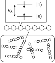
Figure 1: A model of the NMR system for spin-1/2 nuclei.

Standard quantum algorithms are designed to work with a pure-state input. In contrast, there are a few quantum algorithms for the model of deterministic quantum computation with a single pure qubit (DQC1) Knill and Laflamme (1998) and similar models, including one for prime factorization Parker and Plenio (2000) (an extension of Shor’s algorithm Shor (1997)); those are designed to work with a highly mixed state, even with an input string that comprises a single pure qubit (namely, an initialized qubit) and the rest qubits in a maximally mixed state. As the family of DQC1 models does not provide all the replacements of standard quantum algorithms, initialization of many qubits for ensemble quantum computers is still of importance.

There are two types of initialization methods: one is averaging (e.g., effective pure states Knill et al. (1998)); another is data compression. The latter has an advantage in respect of scalability because the former needs resources growing exponentially in $n$ while the latter does not. The boosting scheme proposed by Schulman and Vazirani Schulman and Vazirani ; Schulman and Vazirani (1999) is one of the latter type of methods. Actually, their scheme is a sort of polarization transfer which has been commonly used and thoroughly studied in the realm of NMR spectroscopy as pointed out in Ref. Chang et al. (2001). There have been notable studies of the general upper limit on a polarization enhancement in a polarization transfer (e.g., Refs. Ernst et al. (1987); Sørensen (1990, 1991)). The principle of the boosting scheme is the bias-enhancing permutation as we will see in Sec. II. In the scheme, a quantum circuit Deutsch (1989) properly composed of basic bias-boosting circuits is used for redistributing the biases to generate the block of $l$ cold qubits with biases greater than $\varepsilon_{cold}$ such that

$$\mathrm{Prob}\{0_{1}0_{2}\cdots 0_{l-1}0_{l}\}\gtrapprox\left(\frac{1+\varepsilon_{cold}}{2}\right)^{l}$$ (2)

is large enough to distinguish $|0\rangle^{\otimes l}$ among the signals of $2^{l}$ component states. Their analyses Schulman and Vazirani ; Schulman and Vazirani (1999) resulted in that a compression down to almost the entropic limit is possible (in the limit of large $n$) in $O(n\log n)$ time in the scheme to generate $n(1-o(1))-S$ initialized qubits each of which has bias $1-\exp(-n^{\Theta(1)})$ (which converges to $1$ as $n$ becomes large), where $S$ is the von Neumann entropy von Neumann (1927) of the ensemble . However, this is incorrect unless the original biases are in the neighborhood of $0$ or $1$ . Irrespectively of $n$, the condition of original biases $0<\varepsilon\lnapprox 1$ leads to the circumstance that the probability of a spin being up has classical correlations (classical dependences) with those of other spins within several steps after the beginning of the scheme. Owing to the correlations, $l$ can be much smaller than $n-S$. Especially for the practical setting of $n\leq 10^{3}$, an accurate evaluation of the scheme is of importance since a large mean bias such as $\langle\varepsilon\rangle=0.4$ is required to obtain a sufficient number of initialized qubits Boykin et al. .

In this Paper, we report a numerical analysis of the boosting scheme based on a molecular simulation. Several features of the scheme relating to the total binary entropy have been investigated by using the simulation with the aid of matrix calculations. It has revealed the fact that the number of qubits initialized by the scheme is rather smaller than expected from the von Neumann entropy even for large $n$. This is not a surprise; it is quite possible according to the theory of macroscopic entropy described in Sec. III.

II Boosting scheme

Enhancing the bias $\varepsilon_{i}$ of the $i$th spin is an operation equivalent to increasing the population of a set of molecules whose $i$th spin is up [$\varepsilon_{i}=\varepsilon_{i}(t)$ where $t$ denotes time step]. This is a general conception of initializations for mixed states. As we consider a large number of molecules under a strong static magnetic field such as those in a common liquid- or solid-state NMR system, an $n$-qubit thermal equilibrium state can be written as the density matrix

$$\rho_{eq}=\rho^{eq}_{1}\otimes\rho^{eq}_{2}\otimes\cdots\otimes\rho^{eq}_{n-1}\otimes\rho^{eq}_{n},$$ (3)

where $\rho^{eq}_{i}$ is the density matrix representing the original state of the $i$th spin with the bias $\varepsilon_{i}(0)$:

$$\rho^{eq}_{i}=\begin{pmatrix}\frac{1+\varepsilon_{i}(0)}{2}&0\\ 0&\frac{1-\varepsilon_{i}(0)}{2}\end{pmatrix}.$$ (4)

Let $c_{k}=c_{k}(t)$ denote the population of component state $|k\rangle$ at time step $t$. Then it is also represented as

$$\rho_{eq} = \sum_{k=0}^{2^{n}-1}c_{k}(0)~{}|k\rangle\langle k|$$ (5)

$$= \mathrm{diag}\{c_{0}(0),c_{1}(0),\ldots,c_{2^{n}-2}(0),c_{2^{n}-1}(0)\},$$

where $c_{k}(0)$ are the original populations. The bias of the $i$th spin is enhanced by any unitary operation that permutes a component state with a large population to some component state whose $i$th bit is $0$, since such an operation increases the population of a set of component states whose $i$th bit is $0$:

$$P_{i}=\sum_{k|\text{$i$th bit is 0}}c_{k}.$$ (6)

This population is identical to the probability that the $i$th bit is $0$. Because a component state which consists of a larger number of 0’s and a smaller number of 1’s has a larger population among the $2^{n}$ component states in most cases, any unitary transformation that maps a sufficient number of component states with more than $n/2$ 0’s to those with 0’s in specific $l^{\prime}$ bits enhances the biases of the $l^{\prime}$ spins. The initialization of $l\geq l^{\prime}$ qubits can be realized by a combination of such transformations. When the transformation $U$ is only a product of permutations of component states, as it is nothing but the exchanges of values of $c_{0},\ldots,c_{2^{n}-1}$, the evolved density matrix $\rho=U\rho_{eq}U^{\dagger}$ is still represented as

$$\rho=\sum_{k=0}^{2^{n}-1}c_{k}|k\rangle\langle k|,$$ (7)

although it is often impossible to write $\rho$ in the form of Eq. (3).

In Schulman and Vazirani’s boosting scheme (or simply called the boosting scheme), the total operation for an initialization can be composed of the 3-qubit basic circuits shown in Fig. 2 or the 4-qubit circuit shown in Fig. 3, which perform permutations of component states as mentioned above. It should be noted that these circuits were not distinctly written in the original description of the boosting scheme. Either the 3-qubit circuits or the 4-qubit circuit can be a basic operation of the scheme. If one interprets the original description as it is, one may have the 4-qubit circuit. We, however, use the 3-qubit circuits rather than the 4-qubit circuit because the 3-qubit circuits are better with respect to the rate of initialization. We do not write details about it here, but we will describe a reason in Sec. IV. From now on, we will regard only the 3-qubit circuits as the basic circuits of the scheme.

Figure 2: Basic quantum circuits for constructing an initialization circuit in the boosting scheme. The CNOT gate performs a bit flip (namely, a NOT operation) on the qubit $c$ when $b=1$. The Fredkin gate swaps the qubit $a$ with the qubit $b$ when $c=1$.

Figure 3: Another boosting circuit with a 4-qubit input. The CC-SWAP gate swaps $a$ with $c$ when $bd=11$.

The operation of the basic circuits is illustrated in the truth table of Table 1. By the circuit of Fig. 2(a), a component state with a large population—i.e., a component state in which two of the three qubits are 0—is mapped to a component state in which the first of the three qubits is 0. The probability that the first qubit $a$ is 0 after this basic operation is

$$\mathrm{Prob}\{a=0\}_{out} = \mathrm{Prob}\{000\}_{in}+\mathrm{Prob}\{001\}_{in}$$ (8)

$$+\mathrm{Prob}\{010\}_{in}+\mathrm{Prob}\{100\}_{in},$$

where, for given qubits $a$, $b$, and $c$ (from upper to lower in the circuit) with their binary values $x_{a}$, $x_{b}$, and $x_{c}$,

$$\mathrm{Prob}\{x_{a}x_{b}x_{c}\}=\sum_{k|abc=x_{a}x_{b}x_{c}}c_{k}.$$ (9)

Suppose that no correlation exists among $P_{a}$,$P_{b}$, and $P_{c}$ and that the biases $\varepsilon_{a}$, $\varepsilon_{b}$, and $\varepsilon_{c}$ are positive, in the input. Then the bias of the qubit $a$ in the output of the circuit is

$$\varepsilon^{\prime}_{a}=\frac{1}{2}\left(\varepsilon_{a}+\varepsilon_{b}+\varepsilon_{c}-\varepsilon_{a}\varepsilon_{b}\varepsilon_{c}\right),$$ (10)

and $\varepsilon^{\prime}_{a}$ becomes larger than $\varepsilon_{a}$ under the condition:

$$\varepsilon_{a}<\frac{\varepsilon_{b}+\varepsilon_{c}}{1+\varepsilon_{b}\varepsilon_{c}}.$$ (11)

Similar calculations give the biases for $b$ and $c$ in the same output:

$$\varepsilon^{\prime}_{b}=\frac{1}{2}\left(\varepsilon_{a}+\varepsilon_{b}-\varepsilon_{c}+\varepsilon_{a}\varepsilon_{b}\varepsilon_{c}\right),$$ (12)

$$\varepsilon^{\prime}_{c}=\varepsilon_{b}\varepsilon_{c}.$$ (13)

After the circuit of Fig. 2(a), the bias of the qubit $b$ may be smaller than 0; the circuit of Fig. 2(b) is added to invert the bias in this case.

Table 1: Truth table for the basic circuits in Fig. 2 for the boosting scheme. Here, the input of (b) is the output of (a).

3-qubit boosting
Input	Output of (a)	Output of (b)
000	000	010
001	001	011
010	011	001
011	100	110
100	010	000
101	101	111
110	111	101
111	110	100

In the case where three spins are polarized uniformly with the bias $\varepsilon_{uni}$ in the input, Eq. (10) leads to

$$\varepsilon^{\prime}_{a}=\frac{3}{2}\varepsilon_{uni}-\frac{1}{2}\varepsilon_{uni}^{3}.$$ (14)

Thus, the basic circuits can be used for boosting the biases of target qubits. It is expected that one can achieve the component state $|0\rangle^{\otimes l}$ with a very large population simply by collecting initialized qubits after sufficient steps of application of these circuits to every subgroup which consists of three qubits that satisfy inequality (11) (although the initialization rate is another subject). Equations (10), (12), and (13) may be used for a rough estimation of the behavior of a quantum circuit composed of the basic circuits.

However, the designing of a whole circuit in the boosting scheme is not so simple. At every step in the scheme, one recreates subgroups by picking up every three qubits from the $n$ qubits in the order of their biases, from larger to smaller, so that the condition of inequality (11) is satisfied in almost every subgroup. It is better to avoid applying the basic circuits to those in which the condition is not satisfied or undo it afterward. In order to recreate the subgroups, one has to forecast the biases of qubits correctly, which requires a more precise estimation owing to the following reason: After several steps in the scheme, the bias of a qubit is not independent of those of others, i.e.,

$$\mathrm{Prob}\{ij=00\}\not=P_{i}P_{j}$$ (15)

for a pair of qubits $(i,j)$ in the $n$-qubit string. This is because the ensemble after a CNOT operation on $(i,j)$ is not determined by the biases $(\varepsilon_{i},\varepsilon_{j})$ alone but dependent on the populations $\{c_{k}\}$. The exception is only the case where the original biases are very close to $0$ or $1$. Therefore, the use of independent probabilities for representing spins in constructing the circuit induces inaccuracy for the large size and/or large depth of the circuit. Each molecule has to be dealt with for correct forecasts of biases.

Moreover, even with the forecasts of biases, it is quite possible that the bias of the qubit $a$ is not boosted in some subgroups at almost every step except for several beginning steps in the scheme. This is due to classical correlations among qubits. The condition of inequality (11) is not an accurate condition for the success of bias boosting in a subgroup of correlated qubits. It is nothing but a rough estimation of a correct condition. Thus, one ought to undo the operations that fail in enhancing the biases of target qubits so as to achieve better bias enhancements. The details of the circuit designing based on the forecasts and undo operations are described in Sec. V and Appendix C.

Note that even the circuits that succeed in enhancing the biases alter the amount of correlation. Although the three qubits in each subgroup are nearly equally biased, this does not mean the binomial distribution, i.e., it is not relevant to the independence of the qubits; their biases can be correlated [their individual probabilities given by Eq. (6) can be dependent] to each other. The classical correlations affect the efficiency of initialization—this “efficiency” is not the efficiency in running time nor that in working space—as described in the next section.

III Classical correlations hidden in macroscopic binary entropies

The initialization of an NMR quantum computer with a method that uses a data compression is equivalent to redistributing the binary entropies of qubits (the entropies of macroscopic bits), $\{H_{i}=$ $\frac{1+\varepsilon_{i}}{2}$ $\log_{2}$ $\frac{2}{1+\varepsilon_{i}}$ $+$ $\frac{1-\varepsilon_{i}}{2}$ $\log_{2}$ $\frac{2}{1-\varepsilon_{i}}$$\}$, to create two different blocks of qubits: one has a very small entropy close to $0$ and the other has a very large entropy as illustrated in Fig. 4.

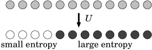
Figure 4: A unitary compression operation $U$ for redistributing the biases to create the block of qubits with small binary entropies and that with large binary entropies.

The block of $l$ qubits with very small binary entropies is used as $|0\rangle^{\otimes l}$. In this respect, an important entropy measure is the sum of the binary entropies of individual qubits: let the effective entropy

$$S_{e}(t)=-\sum_{i=1}^{n}\left(\frac{1+\varepsilon_{i}}{2}\log_{2}\frac{1+\varepsilon_{i}}{2}+\frac{1-\varepsilon_{i}}{2}\log_{2}\frac{1-\varepsilon_{i}}{2}\right),$$ (16)

where $\varepsilon_{i}=\varepsilon_{i}(t)$ is the bias of the $i$th qubit at time step $t$. When the state of the whole $n$-qubit ensemble is represented as a diagonal density matrix, it is given by

$$\varepsilon_{i}=-1+2\sum_{k|\text{$i$th bit is 0}}c_{k}.$$ (17)

On the other hand, when there can be nonzero off-diagonal elements of the density matrix for the system, we have to consider the intrinsic bias defined below rather than the superficial bias that is calculated only from populations. The intrinsic bias of a qubit is a quantity obtained from a unitary diagonalization of the reduced density operator of the qubit. The reduced density operator of the $i$th qubit can be given by the partial trace

$$\tilde{\rho}_{i}=\sum_{k=0}^{2^{n-1}-1}\langle\psi_{k}^{i}|\rho|\psi_{k}^{i}\rangle,$$ (18)

where $\rho=\rho(t)$ is the density matrix for the whole ensemble; $\{|\psi_{k}^{i}\rangle\}=\{|\psi_{0}^{i}\rangle,\ldots,|\psi_{2^{n-1}-1}^{i}\rangle\}$ is a complete orthonormal system of the state space of the rest qubits, such as

$$\begin{split}\{&|0_{1}0_{2}\cdots 0_{i-1}0_{i+1}\cdots 0_{n-1}0_{n}\rangle,\\ &|0_{1}0_{2}\cdots 0_{i-1}0_{i+1}\cdots 0_{n-1}1_{n}\rangle,\\ ~{}~{}~{}~{}~{}~{}&~{}~{}~{}~{}~{}~{}~{}~{}~{}~{}~{}~{}~{}~{}~{}\vdots\hskip 71.0pt,\\ &|1_{1}1_{2}\cdots 1_{i-1}1_{i+1}\cdots 1_{n-1}0_{n}\rangle,\\ &|1_{1}1_{2}\cdots 1_{i-1}1_{i+1}\cdots 1_{n-1}1_{n}\rangle\}.\end{split}$$ (19)

Let ${}^{d}\tilde{\rho}_{i}$ be the matrix with the diagonal elements ${}^{d}c_{i,0}$ and ${}^{d}c_{i,1}$ obtained from a unitary diagonalization of $\tilde{\rho}_{i}$ such that ${}^{d}c_{i,0}\geq{}^{d}c_{i,1}\geq 0$. Then the intrinsic bias of the $i$th qubit is defined as

$$\hat{\varepsilon}_{i}=\frac{{}^{d}c_{i,0}-{}^{d}c_{i,1}}{{}^{d}c_{i,0}+{}^{d}c_{i,1}}.$$ (20)

This definition of intrinsic bias is valid in the sense that its value is independent of a macroscopic spin direction. The direction of the $i$th macroscopic bit $\tilde{\rho}_{i}$ can be modified even with only single-qubit rotation gates. If we restrict the subsequent quantum gates to single-qubit rotations at a particular time step, $\frac{1+\hat{\varepsilon}_{i}}{2}$ is the maximum achievable probability of the $i$th qubit being $0$ after that step. Thus the intrinsic bias is a plain measure of purity of a qubit. Since an initialization is to produce pure qubits, we regard $\hat{\varepsilon}_{i}$ as the actual bias of the $i$th qubit denoted by $\varepsilon_{i}$ in the definition of $S_{e}$: namely, in Eq. (16). When completely initialized qubits are required, $S_{e}$ is a lower bound for the length of the compressed string at a particular time step in an initialization process; $n-S_{e}$ is an upper bound for the number of initialized qubits at that step . $S_{e}$ varies step by step during the initialization.

Now we will see an upper bound for the number of initialized qubits under a realistic condition. Suppose that we do not need completely initialized qubits. Then initialized qubits are allowed to have small binary entropies ($H_{j}$) whose average value ($\frac{1}{l}\sum_{j=1}^{l}H_{j}$) is equal to or less than some real number $\alpha$ ($0\leq\alpha\ll 1$). The total binary entropy of $l$ initialized qubits is equal to or less than $\alpha l$. The block of rest $n-l$ qubits (namely, the compressed string) therefore has the total binary entropy $E\geq S_{e}-\alpha l$. Hence the following inequality holds:

$$n-l\geq E\geq S_{e}-\alpha l.$$ (21)

This leads to

$$l\leq\frac{1}{1-\alpha}(n-S_{e}).$$ (22)

Setting $\beta=\frac{\alpha}{1-\alpha}$, we have

$$l\leq(1+\beta)(n-S_{e})\leq n(1-S_{e}/n+\beta).$$ (23)

In an initialization, even if there is no need of completely initialized qubits, one picks up $l$ cold qubits at the terminal step of it in order to achieve $\mathrm{Prob}\{0_{1}\cdots 0_{l}\}\geq c$ ($0\ll c\leq 1$ is a real number). The value of $c$ is chosen by one’s need. Accordingly, a limitation of the value of $\alpha$ can be estimated as follows: Suppose that the density matrix for a state after initialization has no nonzero off-diagonal element. Let us assume for a moment that one obtains $l$ initialized qubits with independent biases and the rest qubits with biases that may be correlated. If the joint probability of the initialized qubits being zeros is $\mathrm{Prob}\{0_{1}\cdots 0_{l}\}\geq b$ ($0\leq b\leq 1$), then the binary entropies $H_{j}$ for the qubits satisfy the inequality $\sum_{j=1}^{l}H_{j}\leq-l\left[b^{1/l}\log_{2}b^{1/l}+(1-b^{1/l})\log_{2}(1-b^{1/l})\right]$, which is easy to prove by mathematical induction. From the contraposition, if $\sum_{j=1}^{l}H_{j}>-l\left[b^{1/l}\log_{2}b^{1/l}+(1-b^{1/l})\log_{2}(1-b^{1/l})\right]$, then $\mathrm{Prob}\{0_{1}\cdots 0_{l}\}<b$. Therefore, on the present assumption that the biases of initialized qubits are independent, a necessary condition for achieving $\mathrm{Prob}\{0_{1}\cdots 0_{l}\}\geq c$ is that

$$\alpha\leq-c^{1/l}\log_{2}c^{1/l}-(1-c^{1/l})\log_{2}(1-c^{1/l}).$$ (24)

Hence on the present assumption, $\alpha$ tends to $0$ as $l$ increases, and so does $\beta$. Possible values of $\alpha$ and $\beta$ are estimated with inequality (24) by specifying a value of $c$ and assuming that $l$ is in a realistic range. For example, when one needs $c=0.99$ and assumes $l\geq 16$, the values of $\alpha$ and $\beta$ are estimated to be at most $7.59\times 10^{-3}$ and $7.64\times 10^{-3}$ respectively. Indeed, it is, however, possible that $\alpha$ does not tend to $0$ with increasing $l$ to achieve $\mathrm{Prob}\{0_{1}\cdots 0_{l}\}\geq c$ when there are correlations among initialized qubits, but even for such qubits, of course the condition $\alpha\leq-c\log_{2}c-(1-c)\log_{2}(1-c)$ is necessary. Moreover, in the case where one needs the bias of an initialized qubit to converge to $1$ as $n$ grows—e.g. $\varepsilon_{cold}=1-\exp(-n^{x})$ (constant $x>0$)—$\alpha$ and $\beta$ tend to $0$ as $n$ increases—i.e., $\beta=o(1)$ in this case. As we have seen, inequality (23) gives an upper bound for the number of initialized qubits at a particular time step for a realistic initialization. In other words, $S_{e}-\beta(n-S_{e})$ is a lower bound for the length of the compressed string at that step. $\beta$ is a small number, which is estimated to be less than $10^{-2}$ in most of realistic initializations to make several bytes almost pure.

Generally, it is believed to be possible to almost faithfully compress the string of an $n$-qubit ensemble, represented by density matrix $\sigma$, down to the entropic limit with the rate $S(\sigma)/n$ for large $n$ in all kinds of quantum computer including NMR computers (as long as $n$ can be large) because of the analogy to the quantum noiseless coding Schumacher (1995), where

$$S(\sigma)=-\mathrm{Tr}(\sigma\log_{2}\sigma)$$ (25)

is its von Neumann entropy. It is desirable, and believed to be possible, to generate a quantum circuit to accomplish it within the depth of the circuit increasing polynomially in $n$. Indeed any unitary transformation of a density matrix conserves its von Neumann entropy, but it would be probably impossible for a compression scheme which generates a quantum circuit according only to macroscopic quantities of individual qubits, e.g., biases, to do such an ideal compression for an arbitrary input state. For the initialization of NMR quantum computers, this is somewhat clear when we rewrite $S_{e}$ by using the reduced density operators $\{\tilde{\rho}_{i}\}$ of individual qubits. Regarding $\hat{\varepsilon}_{i}$ as the actual bias of the $i$th qubit, we have $H_{i}=S(\tilde{\rho}_{i})$. Consequently, $S_{e}$ is rewritten as

$$S_{e}=\sum_{i=1}^{n}S({\tilde{\rho}_{i}}).$$ (26)

From this notation, it is clear that

$$S_{e}-S=S(\rho~{}\|~{}{\tilde{\rho}_{1}}\otimes\cdots\otimes{\tilde{\rho}_{n}}),$$ (27)

where $S=S(\rho)$, and $S(\rho~{}\|~{}{\tilde{\rho}_{1}}\otimes\cdots\otimes{\tilde{\rho}_{n}})$ is the Umegaki relative entropy Umegaki (1962) of $\rho$ with respect to ${\tilde{\rho}_{1}}\otimes\cdots\otimes{\tilde{\rho}_{n}}$. In general, the Umegaki relative entropy between two density operators $\sigma_{1}$ and $\sigma_{2}$ is defined as

$$S(\sigma_{1}\|\sigma_{2})=\mathrm{Tr}\left(\sigma_{1}\log_{2}\frac{\sigma_{1}}{\sigma_{2}}\right).$$ (28)

It is a measure of the distance (or dissimilarity) between the two operators. On the right-hand side of Eq. (27), $\rho$ represents the whole ensemble while ${\tilde{\rho}_{1}}\otimes\cdots\otimes{\tilde{\rho}_{n}}$ is a tensor product in which correlations are freed (i.e., correlations among ${\tilde{\rho}_{1}},\ldots,{\tilde{\rho}_{n}}$ are obliterated in taking the tensor product). Hence $S_{e}-S$ is a measure of total correlation Henderson and Vedral (2001) of $\rho$: namely, a measure of total correlation of each qubit to the other qubits. Obviously, $S_{e}$ can be much larger than $S$ when there is a growth in the total correlation during the initialization. There is no known way to avoid the creation and growth of correlations among biases when a data-compression circuit is designed by using solely the values of biases at every step instead of those of commonly-used quantities such as the (approximate) populations of possible bit sequences Hamming (1980), the (approximate) length and frequency of patterns in microscopic strings, etc.

Let us consider the boosting scheme, in which every operation is a permutation of diagonal elements in a diagonal density matrix which is originally $\rho_{eq}$ as we have seen in the previous section. Then, clearly, there is no entanglement during and after a bias boosting process; $S_{e}-S$ is a measure of total classical correlation hidden in the macroscopic string (the string which consists of $n$ macroscopic bits ${\tilde{\rho}_{1}},\ldots,{\tilde{\rho}_{n}}$). Thus, in the boosting scheme, an increase in $S_{e}$ measures a growth in the total classical correlation.

In addition, the maximal efficiency of initialization of the macroscopic string is defined by

$$r_{e}=\frac{n-S_{e}^{end}}{n-S},$$ (29)

where $S_{e}^{end}$ is the value of $S_{e}$ after the application of an initialization scheme. This is the ratio of an upper bound for the number of completely initialized qubits that can be achieved by the scheme to the one that is expected from the von Neumann entropy. Similarly, the maximal efficiency of compression of the macroscopic string is defined by

$$r_{c}=S/S_{e}^{end}.$$ (30)

One can evaluate the performance of the scheme by calculating these efficiencies.

IV Growth in the amount of correlation for a basic boosting step

As we have seen in Sec. III, an increase in the amount of correlation must be suppressed to achieve a high initialization rate. In this section, we therefore evaluate the amount of classical correlation generated by a single step of basic boosting circuits.

Suppose that there are three qubits $a$, $b$, and $c$ with uniform bias $\varepsilon$ at thermal equilibrium. For this initial state, the effective entropy defined by Eq. (16) is equal to the von Neumann entropy $S$. Now we apply the 3-qubit circuit of Fig. 2(a) to the qubits. The biases of the qubits become $\frac{3\varepsilon-\varepsilon^{3}}{2}$, $\frac{\varepsilon+\varepsilon^{3}}{2}$, and $\varepsilon^{2}$, respectively. By this operation, classical correlations are induced, and the effective entropy of the output state, $S_{e}^{out}$, is greater than $S$ as shown in Fig. 5. The discrepancy between $S_{e}^{out}$ and $S$ is rather serious for the highly but not completely polarized qubits because $S_{e}^{out}-S$ is fairly large in despite of the small values of $S$.

Similarly, we can evaluate the amount of classical correlation generated by the 4-qubit circuit shown in Fig. 3. When there are 4 input qubits $a$, $b$, $c$, and $d$ with uniform bias $\varepsilon$ at thermal equilibrium, the biases in the output of it are $\frac{3\varepsilon-\varepsilon^{3}}{2}$, $\varepsilon^{2}$, $\frac{\varepsilon+\varepsilon^{3}}{2}$, and $\varepsilon^{2}$, respectively. Thus the effect of bias enhancement looks almost the same as that of the 3-qubit basic circuits. It, however, induces a larger amount of correlation in comparison with the 3-qubit basic circuits. The discrepancy between the effective entropy of the output, $S_{e}^{out}$, and the von Neumann entropy $S$ is shown in Fig. 6.

When one compares the mean discrepancy $(S_{e}^{out}-S)/{n_{b}}$ ($n_{b}=3,4$ is the number of wires) for the 3-qubit circuit with that for the 4-qubit circuit, as shown in Fig. 7, it is clear that the increase in the amount of correlation in one time step is so large that the 4-qubit circuit should not be used as a basic boosting operation. This is the reason why we have chosen the 3-qubit circuits.

Figure 5: Plots of $S_{e}^{out}$, $S$, and $S_{e}^{out}-S$ for $3$ qubits as functions of $\varepsilon$, the uniform original bias of the qubits. $S_{e}^{out}$ is the effective entropy of the output state after one step of the basic circuit shown in Fig. 2(a) and $S$ is the von Neumann entropy of the system.

Figure 6: Plots of $S_{e}^{out}$, $S$, and $S_{e}^{out}-S$ for 4 qubits as functions of $\varepsilon$. $S_{e}^{out}$ is the effective entropy of them after one step of the circuit shown in Fig. 3.

Figure 7: Plots of $(S_{e}^{out}-S)/{n_{b}}$ for the 3-qubit circuit ($n_{b}=3$) and the 4-qubit circuit ($n_{b}=4$) as functions of the original bias $\varepsilon$.

V Automatic circuit generation

A molecular simulation is applied for designing a quantum initialization circuit in the boosting scheme on conventional computers. It is implemented as a circuit composer for the scheme, offering the forecasts of biases during the initialization. The details of the algorithm for the designing are described in Program 1 of Appendix C. In this section, instead of the long program, the brief flowing chart of it is shown in Fig. 8. It utilizes a virtual molecular system to mimic an $n$-qubit ensemble as illustrated in Fig. 1. As we continue to use the same basis $\{|0\cdots 0\rangle,\ldots,|1\cdots 1\rangle\}$, superpositions of multiple computational basis vectors are not produced by the boosting operations. Hence a molecule is represented as an array of $n$ binary digits in the simulation. We consider $N$ molecules that consist of $n$ spins with bias $\varepsilon_{i}$ in the $i$th spin ($N\gg n$).

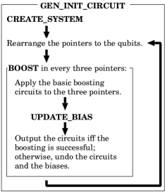
Figure 8: The brief flowing chart of the simulation algorithm of Program 1 to generate an initialization circuit on the basis of the boosting scheme. We show the program in Appendix C.

The outline of Program 1 is as follows: A table of pointers to qubits is used instead of direct handling of them. We consider the subgroups which consist of every three pointers from the upper side to the lower side in the table, although those are not explicitly written in the program. Let frand() be a function which returns a pseudo random real number between $0$ and $1$. This is called $n\cdot N$ times in the procedure CREATE_SYSTEM to set up the virtual molecular system. At each call of frand(), the bit representing the $i$th spin in the $m$th molecule is set to $0$ when $\text{frand()}<(1+\varepsilon_{i}(0))/2$ and set to $1$ otherwise. The desired original biases $\varepsilon_{1}(0),\ldots,\varepsilon_{n}(0)$ are prepared in this way. Then the pointers are arranged in the order of the biases, from the larger to the smaller, in the table (from the upper side to the lower side). The main part of this simulation after the setup is an iteration in the procedure GEN_INIT_CIRCUIT. This iteration contains the following operations: Firstly, BOOST is applied to every subgroup mentioned above. BOOST is the boosting operation for three qubits $a$, $b$, and $c$. We apply the circuit of Fig. 2(a) to them. When the bias of $b$ becomes negative, the circuit of Fig. 2(b) is also applied. The boosting circuits applied to the three qubits are written out if the bias of $a$ is increased by them; otherwise, we undo the boosting. The biases after the boosting are calculated by using UPDATE_BIAS in each call of BOOST. Secondly, we rearrange the table so that the pointers to qubits with larger biases appear in the upper side of it and those with smaller in the lower side. The iteration of above operations is terminated when cold qubits are not newly produced in the last $s_{t}$ steps or when the depth of generated circuits reaches a specified terminal depth of circuits. After this iteration, qubits with very large biases are pointed from pointers located near the top of the table; the component state $|0\rangle^{\otimes l}$ with a very large population is achieved by collecting them.

This algorithm assumes that a CNOT operation can be used with any two qubits in the system. When this is not guaranteed for dispersed qubits, SWAP operations are used to gather them into one location in the molecule. This change is easily realized by arranging the qubits with SWAP gates in GEN_INIT_CIRCUIT instead of arranging only the pointers.

The complexity of the algorithm is $\mathrm{\Theta}(n\cdot N)$ in space and $O(n^{2}\cdot N)$ in time in conventional computers. For a practical use of the simulation for $n\leq 10^{4}$, it would be proper to set $N\simeq 10^{4}n$ and $s_{t}=5+\lfloor 0.1n\rfloor$. Our simulation can be used for generating the circuits up to $10^{4}$ qubits for arbitrary biases within $1$ terabit of memory space.

In addition, the present algorithm is equivalent to the original one proposed by Schulman and Vazirani in Ref. Schulman and Vazirani (1999). In the iteration of the original algorithm, at each step, qubits are rearranged so that qubits with large biases appear first followed by qubits with relatively small biases, discarding those with very low biases. Note that we do not need to discard qubits with very low biases actually. They are dispersed far away from those with large biases by the rearrangement automatically. In the present algorithm, in the iteration, the pointers to qubits are rearranged in the order of the biases. Therefore, it is equivalent to the original one.

Example A

An example of the output circuit from the program of Program 1 is shown in Table 2. It is generated for the 7-pin system, $\mathrm{{}^{1}H\text{-}{}^{1}H\text{-}{}^{1}H\text{-}{}^{1}H\text{-}{}^{1}H\text{-}{}^{1}H\text{-}{}^{1}H}$ with the uniform bias $0.6$. Figure 9 shows that, according to the numerical matrix calculation result, the bias of the first spin is enhanced as it is designed to. Although it appears to be possible to enhance the bias further at a glance, it is impossible for the boosting scheme owing to strong classical correlations among the qubits. An NMR experiment of this bias boosting will be hopefully possible in future.

Table 2: The initialization circuit generated for the spin system, $\mathrm{{}^{1}H\text{-}{}^{1}H\text{-}{}^{1}H\text{-}{}^{1}H\text{-}{}^{1}H\text{-}{}^{1}H\text{-}{}^{1}H}$. The spins are labeled $1,\ldots,7$, from left to right, respectively. The transformations in this table are executed from left to right and upper to lower. X, CN, and Fr read NOT gate, controlled-NOT gate, and Fredkin gate (controlled-SWAP gate), respectively, followed by numbers in parentheses indicating which qubits are handled. In CN($a$,$b$), the control bit is $a$ and the target bit is $b$; in Fr($a$ $b$, $c$), the control bit is $c$ and the target bits are $a$ and $b$.

CN(2,3);X(3);Fr(1 2, 3);X(3);

CN(5,6);X(6);Fr(4 5, 6);X(6);

CN(2,6);X(6);Fr(7 2, 6);X(6);

CN(2,3);X(3);Fr(6 2, 3);X(3);

CN(6,5);X(5);Fr(3 6, 5);X(5);

CN(5,3);X(3);Fr(6 5, 3);X(3);

CN(4,7);X(7);Fr(1 4, 7);X(7);

Figure 9: The result from a matrix calculation for the first example. (a) The original biases of the 7-spin system. (b) Redistributed biases after the operations of Table 2. One of the $\mathrm{{}^{1}H}$ spin biases is boosted under the preset low temperature such that the original bias of the hydrogen is $0.6$, in this matrix calculation.

Example B

The second example is an output circuit for qubits with initially nonuniform biases. The circuit shown in Table 3 is generated for the 9-spin system, $\mathrm{{}^{1}H\text{-}{}^{1}H\text{-}{}^{1}H\text{-}{}^{1}H\text{-}{}^{13}{C}\text{-}{}^{13}{C}\text{-}{}^{13}{C}\text{-}{}^{31}{P}\text{-}{}^{31}{P}}$. We used a modified program to boost mainly the bias of the 5th spin. The numerical matrix calculation of the boosting with the circuit results in an increase in the bias of one of the $\mathrm{{}^{13}C}$ spins as expected from the molecular simulation (Fig. 10). Of course, the effect of the boosting is too small to obtain an initialized qubit in such a small molecule.

Table 3: The initialization circuit generated for the spin system, $\mathrm{{}^{1}H\text{-}{}^{1}H\text{-}{}^{1}H\text{-}{}^{1}H\text{-}{}^{13}{C}\text{-}{}^{13}{C}\text{-}{}^{13}{C}\text{-}{}^{31}{P}\text{-}{}^{31}{P}}$. The spins are labeled $1,\ldots,9$, from left to right, respectively. The notation of the operations in this table is the same as that in Table 2.

CN(6,7);X(7);Fr(5 6, 7);X(7);

CN(9,2);X(2);Fr(8 9, 2);X(2);

CN(6,9);X(9);Fr(7 6, 9);X(9);

CN(1,4);X(4);Fr(2 1, 4);X(4);

CN(6,1);X(1);Fr(9 6, 1);X(1);

CN(4,3);X(3);Fr(7 4, 3);X(3);

CN(4,3);X(3);Fr(9 4, 3);X(3);X(4);

CN(7,8);X(8);Fr(5 7, 8);X(8);

Figure 10: The result from a matrix calculation for the second example. (a) The original biases of the 9-spin system. (b) Redistributed biases after the operations of Table 3. One of the $\mathrm{{}^{13}C}$ spin biases is boosted under the preset low temperature such that the original bias of the hydrogen is $0.8$, in this matrix calculation.

VI Results from simulation

The simulation of Program 1 has been conducted under several different conditions of the original biases and the number of qubits, with the number of virtual molecules $N=5.0\times 10^{6}$. This value of $N$ is large enough to ensure the reliability of the simulation as we show in Appendix A. $\varepsilon_{cold}$ was set to $2\times 0.9^{1/\lceil n-S\rceil}-1$ (this is larger than $0.99$ when $n-S\geq 22$) in Program 1. ($S$ is the von Neumann entropy of a simulated system.) As described in Sec. III, we propose to compute the sum of the binary entropies of individual qubits during the simulation because it is a lower bound for the length of the compressed string at a particular time step $t$, at least approximately, in the boosting scheme. Recall that the effective entropy is thus the total binary entropy given by

$$S_{e}(t)=\sum_{i=1}^{n}\left(\frac{1+\varepsilon_{i}}{2}\log_{2}\frac{2}{1+\varepsilon_{i}}+\frac{1-\varepsilon_{i}}{2}\log_{2}\frac{2}{1-\varepsilon_{i}}\right)$$ (16’)

($\varepsilon_{i}=\varepsilon_{i}(t)$) and that $S_{e}$ can be increased by the growth of classical correlations among qubits in the scheme. At the last step in the simulation, we ignored the preset value of $\varepsilon_{cold}$ and picked up $l$ cold qubits so that the condition of $\mathrm{Prob}\{0_{1}\cdots 0_{l}\}>0.9$ was satisfied; although this does not affect the initialization process itself, nor does it affect the time evolution of the effective entropy. Here we adopt the circuit of Fig. 2(a) as the unit quantum circuit for measuring the depth of circuits constructed by the scheme. In addition, let $\varepsilon$ denote uniform original bias for qubits. We assume that $0\leq\varepsilon\leq 1$ because a negative original bias can be inverted in advance.

The logs recorded during each run of the simulation show that although the von Neumann entropy $S=-\mathrm{Tr}(\rho\log_{2}\rho)$ is preserved, the number of qubits initialized after the boosting operations is much less than $n-S$ because $S_{e}$ is increased in the early steps of the boosting procedure. This is well illustrated as the plots of $S_{e}$ against the depth of the circuits (denoted by $d$) for $1000$ qubits with originally uniform biases, as shown in Fig. 11. For an example, let us take $\varepsilon=0.7$ in the figure. Although the value of the von Neumann entropy is $609.8$, the value of $S_{e}$ at $d=40$ is $806.8$. The number of qubits that can be initialized is reduced from $390$ to $193$ approximately.

The relation of $S_{e}^{end}$ (the terminal value of $S_{e}$) to $S$ was found to be of interest. We plot $S_{e}^{end}/n$ against $S/n$ for several different values of $n$ in Fig. 12. The original biases were set to be uniform and the data were taken for $0\leq\varepsilon\leq 0.975$. It suggests

$$S_{e}^{end}/n\simeq\sqrt{S/n}$$ (31)

for $n\geq 70$. In addition to this relation, it suggests that for $n\geq 70$ and $0\leq\varepsilon\leq 0.65$,

$$S_{e}^{end}/n>\sqrt{S/n},$$ (32)

in consequence of the fact that a value of $S_{e}^{end}/n$ was found to be insensitive to a value of $n\geq 70$ for this range of $\varepsilon$. The figure also shows that the data points of $S_{e}^{end}/n$ for $n=1000$ is slightly closer to the curve of $\sqrt{S/n}$ than those for smaller values of $n$. Furthermore, more than $60\%$ of the increase in $S_{e}$ occurs during $d\leq 5$ when $n=1000$; the number of qubits to which a qubit is classically correlated is nearly $3^{5}=243<1000$ for this depth. Hence the growth in $S_{e}/n$ during $d\leq 5$ is almost unchanged for larger values of $n$. Thus, as $n$ becomes large, $S_{e}^{end}/n$ varies only slightly, getting closer to $\sqrt{S/n}$. Therefore, Eq. (31) for $0\leq\varepsilon\leq 0.975$ and inequality (32) for $0\leq\varepsilon\leq 0.65$ are true for the circuits with larger widths, i.e., they are true for ${}^{\forall}n\geq 70$. Because the data points of $S_{e}^{end}/n$ are in the interval of $[\sqrt{S/n}-0.044,\sqrt{S/n}+0.032]$ when $n=1000$, the relation of $S_{e}^{end}$ to $S$ for $n\geq 1000$ and $0\leq\varepsilon\leq 0.975$ is given by

$$S_{e}^{end}=n\left(\sqrt{S/n}+\delta\right),$$ (33)

where $\delta$ is a real number ($-0.05<\delta<0.04$).

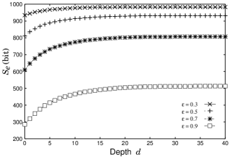
Figure 11: Plots of the effective entropy $S_{e}$ against the depth of circuits from the simulation logs for $n=1000$. The simulation started with qubits with uniform biases. The data points were obtained for the different values of original bias: $\varepsilon=0.3$, $\varepsilon=0.5$, $\varepsilon=0.7$, and $\varepsilon=0.9$.

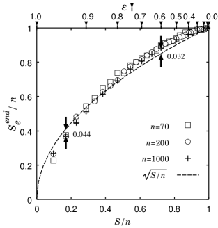
Figure 12: Plots of $S_{e}^{end}/n$ against $S/n$ for the different values of $n$: $n=70$, $n=200$, and $n=1000$. The values of original uniform bias $\varepsilon$ are also shown on the horizontal axis. Each run of the simulation was terminated at the depth of $d=100$. The plots are data points from the simulation, all of which approximately lie on the curve of $S_{e}^{end}/n=\sqrt{S/n}$. The facing arrow pairs indicate the most distant data points from the curve in the vertical direction for $n=1000$, accompanied by the distance values (both upper and lower side).

This phenomenon is originated from the fact that the basic circuits increase the effective entropy of 3 qubits input with independent uniform biases unless their value is $0$ or $\pm 1$ as we have already seen in Fig. 5. In addition, the value of $S_{e}^{end}/n$ is not sensitive to the preset value of $\varepsilon_{cold}$ as long as $\varepsilon_{cold}\geq 0.92$ for $\varepsilon\lessapprox 0.5$ and $\varepsilon_{cold}\geq 0.99$ for $\varepsilon\gtrapprox 0.5$ as shown in Fig. 13. Therefore, the above relations, inequality (32) and Eq. (33), are unchanged even if one presets $\varepsilon_{cold}$ in another way at one’s option as long as $\varepsilon_{cold}$ is suitably large.

Figure 13: Plots of $S_{e}^{end}/n$ against $\varepsilon_{cold}$ for several different values of original uniform bias $\varepsilon$. $n$ was set to $100$ for the data points in this figure.

Moreover, the initialization rate $l/n$ is not rapidly improved by increasing the value of $n$ as shown in Fig. 14, where $l$ is the number of cold qubits picked up at the end of the program. Although $l$ is expected to be close to $n-S_{e}^{end}$ for large values of $n$, only $l\simeq 0.7(n-S_{e}^{end})$ is achieved even when $n=1000$ and $\varepsilon=0.9$. This is due to the increase in the threshold of the bias for cold qubits picked up at the terminal step, since it becomes large for large $n$ in order to avoid reduction in the population of the component state $|0_{1}\cdots 0_{l}\rangle$.

Figure 14: The initialization rate $l/n$ against $n$ for the values of uniform original bias: $\varepsilon=0.3$, $\varepsilon=0.5$, $\varepsilon=0.7$, and $\varepsilon=0.9$. $l$ is the number of cold qubits picked up at the last step in the simulation. For each data point, we chose the largest of 5 samples of $l$ that were calculated with different random seeds.

There are still some other plots of data: The maximal efficiency of initialization, $r_{e}=(n-S_{e}^{end})/(n-S)$, is plotted in Fig. 15. It is not large enough unless the original bias is almost $1$ if we regard the scheme as a classical data compression method.

Figure 15: The maximal efficiency of initialization, $r_{e}=(n-S_{e}^{end})/(n-S)$, for $n=1000$ against the uniform original bias $\varepsilon$. The crosses are data points from the simulation and the curve is the spline fit.

Matrix calculations were conducted to verify the behavior of the automatically generated circuits for $n\leq 13$, indicating the reliability of our molecular simulation. Two of them have been already shown in the examples of Sec. V. The reliability of the simulation is also statistically evaluated in Appendix A. The relation of $S_{e}^{end}$ to $S$ was obtained also for the biases that are originally nonuniform when $n=70$, showing almost the same amount of increase in $S_{e}^{end}$ as that for originally uniform biases (see Appendix B).

One can conclude from the results of our molecular simulation, especially from Eq. (33), that the number of initialized qubits after the application of the boosting scheme is

$$l\leq n\left(1-\sqrt{S/n}-\delta+\beta\right)$$ (34)

for $n\geq 1000$ and $0\leq\varepsilon\leq 0.975$, where $S$ is the von Neumann entropy of the system, $\delta\in(-0.05,0.04)$, and $\beta$ is a small number that has appeared in inequality (23) of Sec. III. $\beta$ is negligible for large $l$, in particular for $n\geq 1000$ and $\varepsilon\gtrapprox 0.3$. When it is required that the bias of an initialized qubit picked up at the terminal step tends to $1$ with increasing $n$, $\beta=o(1)$. In addition, combining one of the results inequality (32) with inequality (23), we find that, for $n\geq 70$ and $0\leq\varepsilon\leq 0.65$,

$$l<n\left(1-\sqrt{S/n}+\beta\right).$$ (35)

VII Discussion

Much work has been done on the theory of quantum data compression of mixed states Schumacher (1995); Holevo ; Horodecki (1998); Jozsa et al. (1998); Horodecki (2000); Nielsen and Chuang (2000); Kramer and Savari . Nevertheless, our numerical analysis is the first evaluation of large quantum circuits actually generated by a compression scheme for ensemble quantum computing as far as the authors know. Calculating an actual compression rate for a specific case is quite another subject than a theoretical proof of a limit to a compression rate. For an initialization of ensemble computers, the string to be compressed is a macroscopic string which is a probabilistic mixture of microscopic strings. It is probably impossible to generate a quantum circuit providing the optimal compression rate for this case as long as only the biases of qubits are referred to at each step of the circuit designing. It would be possible to construct the optimal compression circuit when it is generated by referring to the populations of component states. So far, efficient and effective initialization schemes are those which target the typical sequences Nielsen and Chuang (2000); Kitagawa et al. (2003).

The general difficulty in the evaluation of a quantum data compression scheme is caused by correlations among qubits after multiple-qubit operations. Our program has demonstrated that it does not cost so much resources to simulate a scheme for initial thermal states in which only permutations of component states are used since only classical correlations can be induced. The boosting scheme is one of this special type of compression methods although its initialization rate is not large. There are many polynomial-time classical data compression schemes offering the average code length approximately equal to the Shannon entropy of the original probability distribution for suitably large $n$, e.g., enumerative coding Cover (1973), some of which were reconstructed as quantum algorithms Cleve and DiVincenzo (1996); Braunstein et al. (2000); Chuang and Modha (2000); Langford (2002). A common efficient classical data compression may be used for a more effective initialization as long as the number of required clean qubits of workspace is $\log_{2}[O(\mathrm{poly}(n))]$ Kitagawa et al. (2003). With a proper molecular simulation, a quantum circuit constructed by a classical data compression scheme would be easily evaluated.

To realize a high initialization rate, the value of the total binary entropy $S_{e}$ at the terminal step in an initialization scheme must be nearly equal to that of the von Neumann entropy of the system. In the boosting scheme, as illustrated in Fig. 11, although the growth of $S_{e}$ is a little suppressed, the suppression is not sufficiently strong. The amount of correlation $S_{e}-S$ grows step by step, mainly in the early steps, in the bias boosting process. In other words, a classical string whose macroscopic bits are strongly correlated to each other can only be compressed by the scheme without an increase in the amount of correlation, although such a string does not exist initially in a common NMR system. An effective initialization scheme must have an ability to suppress the growth in the total correlation.

Finally, we have to discuss the curious relation of $S_{e}^{end}$ to $S$ that has been suggested by the simulation results. The relation given by Eq. (31) is simple despite the complicated process of the growth in $S_{e}$. It is difficult to predict the growth without the molecular simulation. Indeed, there are nothing but a few trivial things that support an intuitive interpretation of the relation:
1. $S_{e}^{end}=S$ when $\varepsilon=0$ or $\varepsilon=1$.
2. $S_{e}^{end}$ increases monotonically as $S$ increases, at least approximately.
But there might be also a profound physics in the simple relation, although it is, of course, a result for a special scheme. We have calculated the growth of $S_{e}$ only in the circuits that comprise the basic circuits shown in Fig. 2. It is of interest to examine a growth in the sum of binary entropies in a similar scheme with another basic circuits as well as that in other compression schemes.

VIII Conclusion

A molecular simulation has been demonstrated to evaluate the effectiveness of Schulman and Vazirani’s boosting scheme for the initialization of NMR quantum computers. We have confirmed that a generated quantum circuit will enhance the biases of target qubits as it is designed to. However, our results have also indicated that the scheme is rather inefficient with respect to the initialization rate even for a large number of qubits. When we use 3-qubit basic circuits, the rate is at most approximately $1-\sqrt{S/n}$ even for $n\geq 10^{3}$ as long as $0\leq\varepsilon\leq 0.975$, where $S$ is the von Neumann entropy of a whole $n$-qubit ensemble. This is owing to a large increase in the sum of the binary entropies of individual qubits. This increase means that a large amount of classical correlation is induced in the macroscopic $n$-qubit string. It is to be hoped that an advanced algorithm that suppresses the growth in the amount of correlation will be constructed to improve the rate.

Appendix A Reliability of the simulation

Because our simulation uses a limited number of virtual molecules, there are, to some extent, errors in the output data. The errors comprise both systematic and statistical errors, since the time evolution of the virtual molecular system is deterministic in Program 1 while the setup of the system is dependent on the random seed (see also Appendix C). Here, we present a statistical evaluation of the reliability of the simulation system although the errors are expected to be small in the data used in Sec. VI as we have set the number of molecules suitably large.

In order to evaluate the reliability, the average of sample values of $S_{e}^{end}$ was plotted against the number of molecules, $N$, as shown in Fig. 16. $S_{e}^{end}$ is the value of the effective entropy at the depth of $d=100$ as no further increase in $S_{e}$ was found at larger depth. Considering the running time of the simulation, we chose the original uniform bias $\varepsilon=0.5$ and the number of qubits, $n=100$. The data were obtained by executing the program 60 times for each value of $N$ with different random seeds. In the figure, the error bars represent 99% confidence intervals associated with each mean.

Figure 16: The average values of $S_{e}^{end}$ (solid squares) against the number of virtual molecules $N$ when $\varepsilon=0.5$ and $n=100$. The error bars represent 99% confidence intervals associated with each mean.

The half width of the confidence interval is smaller than $0.4$ bit for the values of $N\geq 5.0\times 10^{5}$. Because the mean value of $S_{e}^{end}$ was found to be insensitive to the value of $N$ and we used the same number of samples for each data point, this indicates that the systematic errors are negligibly small for such large values of $N$. Along with the growth of $N$, the errors are reduced even further. Moreover, the variance of the samples, $V_{s}$, is less than $0.1~{}\mathrm{bit}^{2}$ when $N\geq 5.0\times 10^{5}$ (Fig. 17). Each value of $V_{s}$ was calculated with the 60 samples of $S_{e}^{end}$ at the corresponding value of $N$. This result shows that we do not need to employ a statistical average value of $S_{e}^{end}$, i.e., a single sample value of $S_{e}^{end}$ is reliable enough, when $N$ is set to such a large number. The non-averaged sample values of $S_{e}^{end}$ used in Sec. VI are reliable since we have set $N=5.0\times 10^{6}$.

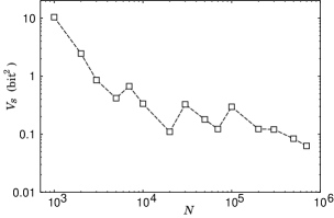
Figure 17: Plots of $V_{s}$ against the number of virtual molecules $N$. $V_{s}$ is the variance of the sample values of $S_{e}^{end}$ at each value of $N$. The sample values are the same as those used in Fig. 16.

Appendix B Initialization for nonuniform original biases

We believe that the initialization for qubits with nonuniform biases is as effective as that for qubits with uniform biases, in the boosting scheme. Consider $n$ qubits in the structure $\cdots\text{-A-B-A-B-A-B-}\cdots$ where $n$ is even; A and B represent the atom with original bias $\varepsilon_{A}\geq 0$ and that with $\varepsilon_{B}\geq 0$, respectively. The initialization for this structure is equivalent to the one for the structure $\text{A-A-}\cdots\text{-A-A-B-B-}\cdots\text{-B-B}$ since we arrange the pointers to the qubits in the order of the biases.

When $\varepsilon_{A}\gg\varepsilon_{B}$ (i.e., $0\leq\varepsilon_{B}\ll 1$), a pointer to A is rarely grouped with a pointer to B in early time steps in the scheme; the increase in the effective entropy $S_{e,AB}$ occurs separately in $\text{A-A-}\cdots\text{-A-A}$ and in $\text{B-B-}\cdots\text{-B-B}$. Together with Eq. (31), this leads to that the terminal value of $S_{e,AB}$ is given by

$$S_{e,AB}^{end}\simeq\frac{n}{2}\sqrt{2S^{orig}_{A\cdots A}/n}+\frac{n}{2}\sqrt{2S^{orig}_{B\cdots B}/n},$$ (36)

where $S^{orig}_{A\cdots A}\leq n/2$ and $S^{orig}_{B\cdots B}\leq n/2$ are the von Neumann entropies in the original distribution for $\text{A-}\cdots\text{-A}$ and $\text{B-}\cdots\text{-B}$, respectively. The increase in the effective entropy is smaller than or approximately equal to that for qubits with originally uniform biases, since

$$S_{e,AB}^{end}/n\simeq\frac{1}{\sqrt{2n}}\left(\sqrt{S^{orig}_{A\cdots A}}+\sqrt{S^{orig}_{B\cdots B}}\right)\leq\sqrt{S/n},$$ (37)

where $S=S^{orig}_{A\cdots A}+S^{orig}_{B\cdots B}$. On the other hand, when $\varepsilon_{A}\simeq\varepsilon_{B}$, the increase in the effective entropy is almost the same as that calculated for the originally uniform biases. In this case,

$$S_{e,AB}^{end}\simeq\sqrt{nS}.$$ (38)

Now we utilize the coefficient $\chi$ and set $\varepsilon_{B}=\chi\varepsilon_{A}$ to calculate the increase in the effective entropy in the scheme when $n=70$ for several different values of $\chi$ ($0<\chi\leq 1$). The relation of $S_{e,AB}^{end}$ to $S$ is well depicted in Fig. 18. The figure shows that, as long as $0.1\leq\chi\leq 1$, $S_{e,AB}^{end}$ is not sensitive to the value of $\chi$ and all the points approximately lie on the curve of $S_{e,AB}^{end}=\sqrt{nS}$. Hence, the use of Eq. (38) is justified for $n=70$. One can conclude that the number of initialized qubits is

$$l_{AB}\lessapprox n\left(1-\sqrt{S/n}\right)$$ (39)

for any realistic value of $\chi$ ($0.1\leq\chi\leq 1$). Although the relation has been verified in the structure that comprises two species of qubits, similar results are expected to be given for molecules that consist of atoms with many different original biases.

Figure 18: Plots of $S_{e,AB}^{end}$ against $S$ for $\chi=0.1$, $\chi=0.4$, $\chi=0.7$, and $\chi=1$ when $n=70$.

Appendix C Details of the simulation algorithm

Here, we show the details of the simulation algorithm for the bias boosting scheme in the following program of Program 1, which has been explained in Sec. V.

PROGRAM 1: The simulation algorithm for generating an initialization circuit based on the boosting scheme. Here, frand() is a function that returns a pseudo random real number between $0$ and $1$. A qubit with a bias greater than $\varepsilon_{cold}$ is regarded as a cold qubit.

procedure GEN_INIT_CIRCUIT:
begin
call CREATE_SYSTEM
Create tbl[ ], a table of pointers to individual qubits
(tbl[1] is the uppermost end).
Arrange tbl[ ] so that the pointer to a qubit with a
larger  bias  appears  upper  side  and  that  with  a
smaller appears lower side.
while new cold qubits are obtained in last $s_{t}$ steps
and depth of output circuit $\leq$ preset max-
imum depth; do
$j$ $\leftarrow$ minimum $j$ such that $\varepsilon_{\text{tbl[}j\text{]}}$ $\leq$ $\varepsilon_{cold}$
while $j$ $\leq$ $n$ - 2 do
call BOOST(tbl[$j$], tbl[$j+1$], tbl[$j+2$])
if $\varepsilon_{\text{tbl[}j\text{]}}$ is increased then
Output the circuit applied in the last
call of BOOST procedure with the
indication of handled qubits, tbl[$j$],
tbl[$j+1$], and tbl[$j+2$].
else
Undo the last BOOST.
endif
$j$ $\leftarrow$ $j$ + 3
endwhile
Re-arrange tbl[ ].
Take a log of tbl[ ] and $\varepsilon_{\text{tbl[ ]}}$ for simulation use.
endwhile
end

procedure CREATE_SYSTEM:
Create $N$ molecules. (A molecule consists of $n$ binary digits.)
begin
for $m$ $\leftarrow$ 1 to $N$ do
for $i$ $\leftarrow$ 1 to $n$ do
if frand() $<$ (1 + $\varepsilon_{i}$) / 2 then
$i$th bit of $m$th molecule $\leftarrow$ 0
else
$i$th bit of $m$th molecule $\leftarrow$ 1
endif
endfor
endfor
end

procedure BOOST($a$, $b$, $c$):
begin
Consider the trio, $a$th bit, $b$th bit, and $c$th bit.
for $m$ $\leftarrow$ 1 to $N$ do
Apply Fig. 2(a) to the trio on $m$th molecule.
endfor
call UPDATE_BIAS($a$)
call UPDATE_BIAS($b$)
call UPDATE_BIAS($c$)
if $\varepsilon_{b}$ $<$ 0 then
for $m$ $\leftarrow$ 1 to $N$ do
Apply Fig. 2(b) to the trio on $m$th
molecule.
endfor
call UPDATE_BIAS($b$)
endif
end

procedure UPDATE_BIAS($i$):
begin
$s$ $\leftarrow$ 0
for $m$ $\leftarrow$ 1 to $N$ do
if $i$th bit of $m$th molecule is 0 then
$s$ $\leftarrow$ $s$ + 1
endif
endfor
$p$ $\leftarrow$ $s$ / $N$
$\varepsilon_{i}$ $\leftarrow$ 2 * $p$ - 1
end

References

- Chuang et al. (1998a) I. L. Chuang, N. Gershenfeld, and M. Kubinec, Phys. Rev. Lett. 80, 3408 (1998a).
- (2) D. G. Cory, W. Mass, M. Price, E. Knill, R. Laflamme, W. H. Zurek, T. F. Havel, and S. S. Somaroo, eprint e-print quant-ph/9802018.
- Chuang et al. (1998b) I. L. Chuang, L. M. K. Vandersypen, X. Zhou, D. W. Leung, and S. Lloyd, Nature 393, 143 (1998b).
- Cory et al. (1997) D. G. Cory, A. F. Fahmy, and T. F. Havel, Proc. Nat. Acad. Sci. USA 94, 1634 (1997).
- Gershenfeld and Chuang (1997) N. Gershenfeld and I. L. Chuang, Science 275, 350 (1997).
- Deutsch (1989) D. Deutsch, Proc. R. Soc. London, Ser. A 425, 73 (1989).
- Schumacher (1995) B. Schumacher, Phys. Rev. A 51, 2738 (1995).
- Knill et al. (1998) E. Knill, I. Chuang, and R. Laflamme, Phys. Rev. A 57, 3348 (1998).
-
Schulman and Vazirani (1999)
L. J. Schulman and
U. V. Vazirani, in
Proceedings of the 31st ACM Symposium on
Theory of Computing (STOC’99) (ACM Press, New York,
1999), pp. 322–329, eprint e-print http://www.cs.caltech.edu/~schulman/
http://www.cs.berkeley.edu/~vazirani/. - (10) L. J. Schulman and U. V. Vazirani, e-print quant-ph/9804060.
-
(11)
J. H. Reif,
online preprint
http://www.cs.duke.edu/~reif/paper/qcompress.ps, 1999 (unpublished). - Knill and Laflamme (1998) E. Knill and R. Laflamme, Phys. Rev. Lett. 81, 5672 (1998).
- Parker and Plenio (2000) S. Parker and M. B. Plenio, Phys. Rev. Lett. 85, 3049 (2000).
- Shor (1997) P. W. Shor, SIAM J. Comput. 26, 1484 (1997).
- Chang et al. (2001) D. E. Chang, L. M. K. Vandersypen, and M. Steffen, Chem. Phys. Lett. 338, 337 (2001).
- Sørensen (1990) O. W. Sørensen, J. Magn. Reson. 86, 435 (1990).
- Sørensen (1991) O. W. Sørensen, J. Magn. Reson. 93, 648 (1991).
- Ernst et al. (1987) R. R. Ernst, G. Bodenhausen, and A. Wokaun, Principles of nuclear magnetic resonance in one and two dimensions (Clarendon Press, Oxford University Press, 1987), chap. 4.
- von Neumann (1927) J. von Neumann, Gött. Nachr. pp. 273–291 (1927), in German.
- (20) P. O. Boykin, T. Mor, V. Roychowdhury, F. Vatan, and R. Vrijen, eprint e-print quant-ph/0106093.
- Umegaki (1962) H. Umegaki, Kodai Math. Sem. Rep. 14, 59 (1962).
- Henderson and Vedral (2001) L. Henderson and V. Vedral, J. Phys. A 34, 6899 (2001).
- Hamming (1980) R. W. Hamming, Coding and Information Theory (Prentice-Hall, Englewood Cliffs, NJ, 1980), chap. 4-6.
- (24) A. S. Holevo, eprint e-print quant-ph/9708046.
- Jozsa et al. (1998) R. Jozsa, M. Horodecki, P. Horodecki, and R. Horodecki, Phys. Rev. Lett. 81, 1714 (1998).
- Horodecki (2000) M. Horodecki, Phys. Rev. A 61, 052309 (2000).
- (27) G. Kramer and S. A. Savari, eprint e-print quant-ph/0101119.
- Nielsen and Chuang (2000) M. A. Nielsen and I. L. Chuang, Quantum Computation and Quantum Information (Cambridge University Press, Cambridge, England, 2000), chap. 12, pp. 528–607.
- Horodecki (1998) M. Horodecki, Phys. Rev. A 57, 3364 (1998).
- Kitagawa et al. (2003) M. Kitagawa, A. Kataoka, and T. Nishimura, in Proceedings of the 6th Int. Conf. on Quantum Communication, Measurement and Computing (QCMC’02), edited by J. H. Shapiro and O. Hirota (Rinton Press, Princeton, 2003), pp. 275–280.
- Cover (1973) T. M. Cover, IEEE Trans. Inf. Theory 19, 73 (1973).
- Cleve and DiVincenzo (1996) R. Cleve and D. P. DiVincenzo, Phys. Rev. A 54, 2636 (1996).
- Braunstein et al. (2000) S. L. Braunstein, C. A. Fuchs, D. Gottesman, and H.-K. Lo, IEEE Trans. Inf. Theory 46, 1644 (2000).
- Chuang and Modha (2000) I. L. Chuang and D. S. Modha, IEEE Trans. Inf. Theory 46, 1104 (2000).
- Langford (2002) J. Langford, Phys. Rev. A 65, 052312 (2002).
- Iinuma et al. (2000) M. Iinuma, Y. Takahashi, I. Shaké, M. Oda, A. Masaike, T. Yabuzaki, and H. M. Shimizu, Phys. Rev. Lett. 84, 171 (2000).
- (37) K. Takeda, K. Takegoshi, and T. Terao, J. Phys. Soc. Jpn. 73, 2313 (2004); Chem. Phys. Lett. 345, 166 (2001).
- Anwar et al. (2004) M. S. Anwar, D. Blazina, H. A. Carteret, S. B. Duckett, T. K. Halstead, J. A. Jones, C. M. Kozak, and R. J. K. Taylor, Phys. Rev. Lett. 93, 040501 (2004).
- (39) M. S. Anwar, J. A. Jones, D. Blazina, S. B. Duckett, and H. A. Carteret, e-print quant-ph/0406044.
- Smith et al. (1994) S. A. Smith, T. O. Levante, B. H. Meier, and R. R. Ernst, J. Magn. Reson. 106a, 75 (1994).